Brane embeddings in sphere submanifolds

Nikos Karaiskos, Konstadinos Sfetsos and Efstratios Tsatis
Department of Engineering Sciences, University of Patras

26110 Patras, Greece

$\{$nkaraiskos, sfetsos, etsatis$\}$@upatras.gr

Synopsis

Wrapping a D(8-p)-brane on $AdS_{2}$ times a submanifold of $S^{8-p}$ introduces point-like defects in the context of AdS/CFT correspondence for a Dp-brane background. We classify and work out the details in all possible cases with a single embedding angular coordinate. Brane embeddings of the temperature and beta-deformed near horizon D3-brane backgrounds are also examined. We demonstrate the relevance of our results to holographic lattices and dimers.

1 Prolegomena

When branes wrap internal manifolds, they have the tendency to shrink. However, they can be stabilized by turning on a worldvolume gauge field with a quantized flux. A pioneering example of such flux stabilization of D-branes was presented in [1] for the wrapping of a probe D2-brane inside an $SU(2)$ group manifold and a connection with results from an exact CFT approach was also made. There have been numerous works in the literature considering brane embeddings in various backgrounds and dimensions [2]-[7] (and references therein). In particular, the authors of [4] considered configurations where a D(8-p)-background wraps an $\mathbb{S}^{7-p}$ inside an $\mathbb{S}^{8-p}$ in the background of a Dp-brane. The stabilization occurs at quantized values of the equatorial angle of the bigger sphere. This result, besides being aesthetically beautiful, is also relevant in a holographic approach to condensed matter lattices and dimer systems [8].

Motivated by these works we realized that for generic values of $p$ there are more embedding possibilities even when one considers the simplest case of one embedding coordinate. Instead of $\mathbb{S}^{7-p}$, one could also select other submanifolds of $\mathbb{S}^{8-p}$ whose isometry groups are essentially given by subgroups of $SO(9-p)$, the latter being the isometry group of $\mathbb{S}^{8-p}$. These submanifolds are presented in Table 1 for $p=0,1,\dots,5$. The coloring is introduced for later convenience.

Table 1: Submanifolds of $\mathbb{S}^{8-p}$.

$p=0$	$\mathbf{S^{7}}$,   $\mathbf{S^{3}\times S^{4}}$,   $\mathbf{S^{2}\times S^{5}}$,   $\mathbf{S^{1}\times S^{6}}$
$p=1$	$\mathbf{S^{6}}$,   $\mathbf{S^{3}\times S^{3}}$,   $\mathbf{S^{2}\times S^{4}}$,    $\mathbf{S^{1}\times S^{5}}$,   $\mathbf{CP^{3}}$
$p=2$	$\mathbf{S^{5}}$,   $\mathbf{S^{2}\times S^{3}}$,   $\mathbf{S^{1}\times S^{4}}$
$p=3$	$\mathbf{S^{4}}$,   $\mathbf{S^{2}\times S^{2}}$,   $\mathbf{S^{1}\times S^{3}}$,   $\mathbf{CP^{2}}$
$p=4$	$\mathbf{S^{3}}$,   $\mathbf{S^{1}\times S^{2}}$
$p=5$	$\mathbf{S^{2}}$,   $\mathbf{S^{1}\times S^{1}}$

This paper is organized as follows: In section 2 we minimize the action of the brane probe and calculate the semi-classical energy for each one of the aforementioned configurations. In general, the energy depends on the ratio of the flux units $n$ of the worldvolume gauge field to the number of the Dp-branes $N$, that we stack together to form the background. For a given value of $p$ these energies depend on the specific submanifold that is wrapped.

In section 3 we present brane embeddings in $\beta$-deformed backgrounds [9]. In this case it turns out that the $\gamma$ dependence of the deformation drops out completely in the probe computation. Pertaining to the $\sigma$-deformation, which involves an S-duality, we formulated the problem mathematically, but we were not able to find minimal configurations explicitly due to its complexity.

In section 4, we turn on the temperature and examine its effect on the stability of our constant embeddings. We conclude, by considering a small fluctuation analysis, that these are perturbatively stable.

In section 5 we apply our results in the context of holographic lattices and dimers. We show that the free energy, and hence the physical behavior of the systems, is sensitive in a simple manner to the different wrappings we have constructed. Finally, in section 6 we present concluding remarks and comment on future directions.

2 Brane embeddings in Ramond-Ramond backgrounds

The geometry created by a stack of $N$ coincident Dp-branes in the near-horizon region is described by the ten-dimensional metric [10]

$$ds^{2}=\left(\frac{r}{R}\right)^{\frac{7-p}{2}}(-dt^{2}+d\vec{x}^{2}_{||})+\left(\frac{R}{r}\right)^{\frac{7-p}{2}}(dr^{2}+r^{2}d\Omega_{8-p}^{2})\ ,$$ (1)

where $d\Omega_{p}^{2}$ is generally the line element of a unit $p$-sphere and the parameter $R$ is given by

$$R^{7-p}=N~{}g_{s}~{}2^{5-p}~{}\pi^{\frac{5-p}{2}}~{}(\alpha^{\prime})^{\frac{7-p}{2}}~{}\Gamma(\tfrac{7-p}{2})\ .$$ (2)

The background is also supported by a dilaton, $\Phi(r)$ and a non-zero Ramond–Ramond (RR) field strength $F_{(8-p)}$ given by

$$e^{-\Phi(r)} = \left(\frac{R}{r}\right)^{\frac{(7-p)(p-3)}{4}}\ ,$$ (3)

$$F_{(8-p)} = (7-p)R^{7-p}~{}\textrm{Vol}(\mathbb{S}^{(8-p)})=\textrm{d}C_{(7-p)}\ ,$$ (4)

where Vol$(\mathbb{S}^{(8-p)})$ denotes the volume form of the unit $p$-sphere and $C_{(7-p)}$ is the RR potential. We split the $(8-p)$ spherical coordinates as $(\theta,\phi_{1},\dots,\phi_{7-p})$ and let $\theta$ and $\vec{x}_{\parallel}$ be the embedding coordinates of the probe brane.

We concentrate first to the cases corresponding to the entries of the Table 1 that involve solely spheres. For these cases the metric of the compact space will have the form

$$d\Omega_{8-p}^{2}=d\theta^{2}+\cos^{2}\theta~{}d\Omega_{q}^{2}+\sin^{2}\theta~{}d\Omega_{7-p-q}^{2}\ ,\qquad q=0,1,\dots,{\left[7-p\over 2\right]}\ .$$ (5)

This parametrization of the metric corresponds to splitting the ${\bf 9-p}$ representation of the symmetry group $SO(9-p)$ under the subgroup $SO(q+1)\times SO(8-p-q)$ as ${\bf(9-p)\to(q+1,1)\oplus(1,8-p-q)}$. The variable $\displaystyle\theta\in[0,{\pi\over 2}]$, unless $q=0$ in which case $\theta\in[0,\pi]$. Consequently, the RR potential will be written as

$$C_{(7-p)}=R^{7-p}~{}f(\theta)~{}\omega_{(7-p)}\ ,$$ (6)

where

$$\omega_{(7-p)}=d{\rm Vol}(\mathbb{S}^{q})\wedge d{\rm Vol}(\mathbb{S}^{7-p-q})=\sqrt{h}d\phi_{1}\wedge d\phi_{2}\dots d\phi_{7-p}\ .$$ (7)

The corresponding volume is

$$\mathbb{V}_{\mathcal{M}}=\int_{\mathcal{M}}d^{7-p}\phi\sqrt{h}=\frac{4\pi^{\frac{9-p}{2}}}{\Gamma\left(\frac{1+q}{2}\right)\Gamma\left(\frac{8-p-q}{2}\right)}\ .$$ (8)

For $q=0$ we should divide this formula by two since the general expression for ${\rm Vol}(\mathbb{S}^{q})$ gives $2$ for $q=0$. The function $f(\theta)$ is given for $q\neq 0$ by

$$f(\theta)=\frac{7-p}{8-p-q}(\sin\theta)^{8-p-q}~{}{}_{2}F_{1}\left(\frac{1-q}{2},4-\frac{p+q}{2},5-\frac{p+q}{2},\sin^{2}\theta\right)\ ,$$ (9)

and for $q=0$ by

$$f(\theta)=2^{8-p}\frac{7-p}{8-p}\left(\sin\tfrac{\theta}{2}\right)^{8-p}~{}{}_{2}F_{1}\left(\frac{p}{2}-3,4-\frac{p}{2},5-\frac{p}{2},\sin^{2}\tfrac{\theta}{2}\right)\ .$$ (10)

This difference originates from the two different ranges that the angular variable $\theta$ takes, as mentioned above. Note also that this is not the most general form for the RR potential, but it is the only one consistent for the particular embedding that we will consider in this article.

The D(8-p)-brane probe is described by the sum of a Dirac-Born-Infeld (DBI) and a Wess-Zumino (WZ) term

$$S=-T_{8-p}\int d^{9-p}\sigma e^{-\Phi}\sqrt{-\textrm{det}(\hat{g}+F)}+T_{8-p}\int C_{(7-p)}\wedge F\ ,$$ (11)

where $\hat{g}$ is the induced metric on the brane, $F$ is an abelian gauge field strength living on the world-volume of the brane and

$$T_{8-p}=(2\pi)^{p-8}~{}(\alpha^{\prime})^{\frac{p-9}{2}}~{}(g_{s})^{-1}\ ,$$ (12)

is the tension of the probe brane. The integration is performed over the world-volume coordinates of the brane which are taken to be $\sigma^{\alpha}=(t,r,\phi_{1},\dots,\phi_{7-p})$. In general, the embedding coordinate may depend on any world-volume coordinate. Here, we shall restrict ourselves to the case where $\theta$ depends only on the radial coordinate, which is also consistent with the form of the RR potential (6). Since the WZ term acts as a source term for the abelian gauge field strength $F$, the latter one is constrained to be $F=F_{tr}~{}dt\wedge dr$. We also set the spacelike worldvolume coordinates $\vec{x}_{||}$ to constants which is consistent with their equations of motion.

Given the above conditions the probe brane action assumes in general the form

$$S=\int_{\mathcal{M}}d^{7-p}\phi\int dtdr\mathcal{L}(\theta,F)\ ,$$ (13)

where the Lagrangian density is computed to be

$$\mathcal{L}(\theta,F)=-T_{8-p}R^{7-p}\sqrt{h}\left[\frac{f^{\prime}(\theta)}{7-p}\sqrt{1-F_{tr}^{2}+r^{2}\theta^{\prime 2}}-f(\theta)F_{tr}\right].$$ (14)

By varying the Lagrangian density with respect to the worldvolume gauge potentials $A_{t}$ and $A_{r}$, one observes that

$$\frac{\partial\mathcal{L}}{\partial F_{tr}}={\rm const}\ .$$ (15)

Then, it turns out that the gauge field assumes the form

$$F_{tr}=\frac{f^{\prime\prime}(\theta)}{\sqrt{(7-p)^{2}(f^{\prime}(\theta))^{2}+(f^{\prime\prime}(\theta))^{2}}}\ .$$ (16)

In order to attribute physical meaning to this constant, we consider the coupling of our system to fundamental strings [4]. This is achieved by replacing $F$ with $F-B$ in $\mathcal{L}$, where $B$ is the Kalb–Ramond field. By expanding, at first order in $B$ we pick out a term of the form

$$\int_{\mathcal{M}}d^{7-p}\phi\int dtdr~{}\frac{\partial L}{\partial F_{tr}}~{}B_{tr}\ .$$ (17)

We can interpret the coefficient in front of $B_{tr}$ as a charge ($n$ units of $T_{f}$) that multiplies the Kalb-Ramond potential of the fundamental string. Therefore, the fundamental strings “feel” a potential in this background, whose strength is proportional to their number, $n$, and their tension $T_{f}=1/(2\pi\alpha^{\prime})$. Consequently, one writes

$$\int_{\mathcal{M}}d^{7-p}\phi~{}\frac{\partial\mathcal{L}}{\partial F_{tr}}=nT_{f}\ ,\qquad n\in\mathbb{Z}\ .$$ (18)

In order to find semi-classical minima of the embeddings, solving the equations of motion arising from the Lagrangian density would suffice. However, since we are also interested in computing the energies of our configurations, we will obtain the minima through the Hamiltonian procedure. By performing a Legendre transformation, which actually removes the WZ part, the Hamiltonian of the system is given by

$$H=\int_{\mathcal{M}}d^{7-p}\phi\int dtdr\left[\frac{\partial\mathcal{L}}{\partial F_{tr}}F_{tr}-\mathcal{L}\right]\ .$$ (19)

Using the explicit form of the Lagrangian (14) and the quantization condition (18) the Hamiltonian becomes

$$H=\lambda NT_{f}\int dtdr\sqrt{1+r^{2}\theta^{\prime 2}}\sqrt{\left(\frac{f^{\prime}(\theta)}{7-p}\right)^{2}+\Big{(}\nu\lambda^{-1}-f(\theta)\Big{)}^{2}}\ ,$$ (20)

where we have defined

$$\nu={n\over N}\ ,\qquad\lambda=\frac{\Gamma\left(\tfrac{7-p}{2}\right)}{\Gamma\left(\tfrac{8-p-q}{2}\right)\Gamma\left(\frac{1+q}{2}\right)}\ .$$ (21)

Since the origin of the constant $\lambda$ is $\mathbb{V}_{\mathcal{M}}$, it turns out that, for reasons explained below (8), for $q=0$ we should divide the above formula by two. It is obvious from the expression for $H$ that it is consistent to look for constant $\theta$ configurations, since in this case the $r$-dependence drops out. Setting $\theta^{\prime}=0$ and requiring $\partial H/\partial\theta=0$ gives the condition

$$f^{\prime\prime}(\theta)=(7-p)^{2}(\nu\lambda^{-1}-f(\theta))\ .$$ (22)

As one can see in Table 2 in some cases, depending on the specific values for $p$ and $q$, this equation admits an exact solution $\theta(\lambda)$, but in general it can only be solved numerically. In the rest of the paper, in order to avoid a plethora of symbols, we will denote by $\theta$ the solution of (22). The energy density is defined by

$$H=\int dr~{}\mathcal{E}\ .$$ (23)

For general values of $p$ and $q$ it is given by

$$\mathcal{E}_{p,q}=\lambda NT_{f}\sqrt{(\cos\theta)^{2q}(\sin\theta)^{2(7-p-q)}+\left(\nu\lambda^{-1}-f(\theta)\right)^{2}{}}\ .$$ (24)

For the case where a one-cycle is manifest, that is $q=1$, the above formula as well as the one for the minima have a much simpler form given by

$$\sin\theta=\left(\tfrac{7-p}{6-p}~{}\nu\right)^{\frac{1}{5-p}},\qquad\mathcal{E}_{p,1}=NT_{f}\sqrt{\nu^{2}+(\sin\theta)^{12-2p}-2\nu(\sin\theta)^{7-p}}.$$ (25)

Noting that $f(0)=0$ and $f({\pi\over 2})=\lambda^{-1}$, we find the limiting behaviors

$$\mathcal{E}_{p,q}=nT_{f}+{\mathcal{O}}(\nu^{2}),\qquad\mathcal{E}_{p,q}=(N-n)T_{f}+{\mathcal{O}}(1-\nu)^{2}\ .$$ (26)

The results of our computations regarding the minima and the corresponding energies are summarized in the Table 2 below. In all cases, the angle $\theta$ ranges from 0 to $\pi/2$. We have also included two more cases, apart from the products of spheres, which arise for odd values of $p$, by writing the $\mathbb{S}^{8-p}$ as a $U(1)$ bundle over $\mathbb{CP}^{\frac{7-p}{2}}$. We use the conventions of [11] and [12] for the $\mathbb{CP}^{2}$ and $\mathbb{CP}^{3}$, respectively. The normalizations for the metrics are such that $R_{\mu\nu}=\frac{16}{p+1}~{}g_{\mu\nu}$ (for the values $p=1$ and $p=3$ that are of interest to us).

Table 2: Minima and energies

–	Cycles	Algebraic equations for minima	$\mathcal{E}_{p,q}$ in units of $NT_{f}$
	$\mathbb{S}^{3}\times\mathbb{S}^{4}$	$-90\sin\theta+25\sin 3\theta+3\sin 5\theta=-112\nu$	$\mathcal{E}_{0,3}$
$p=0$	$\mathbb{S}^{2}\times\mathbb{S}^{5}$	$450\cos\theta+25\cos 3\theta-27\cos 5\theta=448(1-\nu)$	$\mathcal{E}_{0,2}$
	$\mathbb{S}^{1}\times\mathbb{S}^{6}$	$\sin\theta=\left(\frac{7}{6}\nu\right)^{1/5}$	$\nu\sqrt{1-\frac{35}{36}\left(\frac{7}{6}\nu\right)^{2/5}}$
	$\mathbb{S}^{3}\times\mathbb{S}^{3}$	$\sin\theta=\nu^{1/2}$	$\nu(1-\nu)$
$p=1$	$\mathbb{S}^{2}\times\mathbb{S}^{4}$	$18\pi\nu+8\sin 2\theta+5\sin 4\theta=36\theta$	$\mathcal{E}_{1,2}$
	$\mathbb{S}^{1}\times\mathbb{S}^{5}$	$\sin\theta=\left(\frac{6}{5}\nu\right)^{1/4}$	$\nu\sqrt{1-\frac{24}{25}\left(\frac{6}{5}\nu\right)^{1/2}}$
	$\mathbb{CP}^{3}$	as above	as above
$p=2$	$\mathbb{S}^{2}\times\mathbb{S}^{3}$	$\cos\theta=\frac{-2^{1/3}+(5-5\nu+\sqrt{27-50\nu+25\nu^{2}})^{2/3}}{2^{2/3}(5-5\nu+\sqrt{27-50\nu+25\nu^{2}})^{1/3}}$	$\mathcal{E}_{2,2}$
	$\mathbb{S}^{1}\times\mathbb{S}^{4}$	$\sin\theta=\left(\frac{5}{4}\nu\right)^{1/3}$	$\nu\sqrt{1-\frac{15}{32}\left(\frac{25}{2}\nu^{2}\right)^{1/3}}$
	$\mathbb{S}^{2}\times\mathbb{S}^{2}$	$\theta=\frac{\pi}{2}\nu$	$\frac{1}{\pi}\sin\pi\nu$
$p=3$	$\mathbb{S}^{1}\times\mathbb{S}^{3}$	$\sin\theta=\left(\frac{4}{3}\nu\right)^{1/2}$	$\nu\sqrt{1-\frac{32}{27}\nu}$
	$\mathbb{CP}^{2}$	as above	as above
$p=4$	$\mathbb{S}^{1}\times\mathbb{S}^{2}$	$\sin\theta=\frac{3}{2}\nu$	$\nu\sqrt{1-\frac{27}{16}\nu^{2}}$
$p=5$	$\mathbb{S}^{1}\times\mathbb{S}^{1}$	$\theta=0$  or  $\theta=\frac{\pi}{2}$	singular solutions

We should clarify two subcases of the above table. Firstly, the results for the $\mathbb{CP}^{2}$ and the $\mathbb{S}^{1}\times\mathbb{S}^{3}$ submanifolds coincide. This happens because the wrapping in the first case involves the $U(1)$ fiber with group structure $\mathbb{S}^{1}$ and a submanifold inside $\mathbb{CP}^{2}$, which has a similar structure with $\mathbb{S}^{3}$. The same happens with the results for the $\mathbb{CP}^{3}$ and the $\mathbb{S}^{1}\times\mathbb{S}^{5}$ submanifolds. Secondly, for $p=5$ we have the solutions $\theta=0$ and $\theta=\frac{\pi}{2}$ which correspond to the collapse of the D-brane at the poles of the 3-sphere, thus rendering them singular. We also note that we omit the respective equations that give the minima and energies for the submanifolds $\mathbb{S}^{7-p}\subset\mathbb{S}^{8-p}$, which can be found in [4].

Having obtained the energies for the various values for $p$, we plot them together with the energies found in [4] in the following five Figures. The colors (black, blue, purple and red) correspond to the entries with the same colors in Table 1. The energies are plotted as functions of the ratio $\nu$, in units of $NT_{f}$. Curves with the same value for $p$, but a different one for $q$, might intersect. We also use the obvious notation $(q\perp q^{\prime},\nu)$.

We observe from the figures below, that for a given value of $p$, the maximally symmetric submanifolds corresponding to $q=0$ have the lowest energy. When the submanifold in consideration includes an $\mathbb{S}^{1}$ or a $\mathbb{CP}$ space, the ratio $\nu$ cannot exceed the value $\displaystyle{6-p\over 7-p}$ found from (25). At this maximum value, the corresponding value of the energy density is $\displaystyle{1\over 7-p}$.

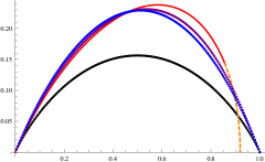
Figure 1: Submanifolds for $p=0$. We have: ($1\!\perp\!2$, $0.46$), ($1\!\perp\!3$, $0.47$) and ($2\!\perp\!3$, $0.48$).

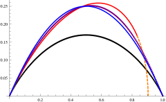
Figure 2: Submanifolds for $p=1$. We have: ($1\!\perp\!2$, $0.49$), ($1\!\perp\!3$, $0.47$) and ($2\!\perp\!3$, $0.51$).

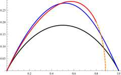
Figure 3: Submanifolds for $p=2$. We have: ($1\!\perp\!2$, $0.48$).

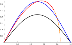
Figure 4: Submanifolds for $p=3$. We have: ($1\!\perp\!2$, $0.50$).

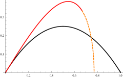
Figure 5: Submanifolds for $p=4$.

The stability of the configurations is ensured by performing a small fluctuation analysis of the fields around the minima. We postpone the analysis until section 4, where a finite temperature is also introduced.

3 Brane embeddings in deformed backgrounds

In this section we consider brane embeddings inside $\beta$-deformed background solutions of type-IIB supergravity [9]. We begin with the $\gamma$-deformation of the $AdS_{5}\times\mathbb{S}^{5}$ background for which the $AdS_{5}$ part of the metric remains the same, while the metric of the $\gamma$-deformed 5-sphere is written as

$$d\Omega_{5,\gamma}^{2}=\sum_{i=1}^{3}(d\mu_{i}^{2}+\mathcal{G}\mu_{i}^{2}d\phi_{i}^{2})+\mathcal{G}R^{4}\gamma^{2}\mu_{1}^{2}\mu_{2}^{2}\mu_{3}^{2}(\sum_{i}d\phi_{i})^{2}\ ,$$ (27)

where

$${\cal{G}}^{-1}=1+R^{4}\gamma^{2}(\mu_{1}^{2}\mu_{2}^{2}+\mu_{2}^{2}\mu_{3}^{2}+\mu_{3}^{2}\mu_{1}^{2})$$ (28)

and $(\mu_{1},\mu_{2},\mu_{3})\equiv(\cos\theta,\sin\theta\cos\psi,\sin\theta\sin\psi)$. The NS sector of the background includes a dilaton and a Kalb–Ramond two-form, given by

$$e^{2\Phi} = \mathcal{G}e^{2\Phi_{0}}$$ (29)

$$B_{NS} = \gamma R^{4}\mathcal{G}(\mu_{1}^{2}\mu_{2}^{2}d\phi_{1}\wedge d\phi_{2}~{}~{}\textrm{+ cyclic})$$ (30)

and the RR potential and field strengths

$$C_{2} = -4\gamma R^{4}w_{1}\wedge(d\phi_{1}+d\phi_{2}+d\phi_{3})\ ,\qquad\textrm{with}~{}~{}dw_{1}=\tfrac{1}{2}\cos\theta\sin^{3}\theta\sin 2\psi d\theta\wedge d\psi\ ,$$ (31)

$$C_{4} = 4R^{4}(w_{4}+\mathcal{G}w_{1}\wedge d\phi_{1}\wedge d\phi_{2}\wedge d\phi_{3})\ ,\qquad\textrm{Vol}(AdS_{5})=dw_{4}\ ,$$ (32)

$$F_{5} = 4R^{4}(\textrm{Vol}(AdS_{5})+\mathcal{G}~{}\textrm{Vol}(\mathbb{S}^{5}))\ ,\qquad\textrm{Vol}(\mathbb{S}^{5})=dw_{1}\wedge d\phi_{1}\wedge d\phi_{2}\wedge d\phi_{3}\ .$$ (33)

We consider D5-brane embeddings in this deformed background. The brane will wrap the four angles of the deformed sphere so that the world-volume coordinates will be $(t,r,\psi,\phi_{i})$ and the embedding coordinates are taken as $\vec{x}_{||}={\rm const.}$ and $\theta=\theta(r)$. As before, we also turn on an Abelian world-volume gauge field strength $F_{tr}$. The action of the brane probe is given by a sum of a DBI and a WZ term. Some extra care is needed since there are new terms arising from the induced Kalb–Ramond field and the RR potentials. The action assumes the generic form

$$S=-T_{5}\int_{D5}e^{-\hat{\Phi}}\sqrt{P[g]+\cal{F}}+T_{5}\int_{D5}\sum_{p}C_{p}\wedge e^{\cal{F}}\ ,$$ (34)

where $\mathcal{F}$ is given by $\mathcal{F}=F-P[B]$, with $F$ and $P[B]$ being the world-volume field strength and the pullback of the Kalb-Ramond potential respectively. After performing the computation, the action for the D5-brane reads

$$S=-\frac{T_{5}R^{4}}{2}\int d\psi d^{3}\phi\sin 2\psi\int dtdr(\cos\theta\sin^{3}\theta\sqrt{1-F_{tr}^{2}+r^{2}\theta^{\prime 2}}-F_{tr}\sin^{4}\theta)\ .$$ (35)

The entire $\gamma$-dependence has dropped out completely due to non-trivial cancellations in the DBI and WZ terms, separately. In fact, this action is exactly the same as that computed for the $p=3$ and $q=1$ case in which the D5-brane wraps the $\mathbb{S}^{1}\times\mathbb{S}^{3}$ submanifold of $S^{5}$. Indeed, one may check that the above Lagrangian falls into the generic family (14) with $f(\theta)=\sin^{4}\theta$, which is the correct function appearing in the RR potential for the aforementioned case.

3.1 Embeddings in the $\sigma$-deformed background

One may also consider a more general deformation of the background, by performing an S-duality in the theory [9]. Apart from $\gamma$, the resulting background depends also on $\sigma$ which is an additional scaleless parameter. Searching for D5-brane embeddings, we choose the embedding coordinates $\vec{x}_{||}={\rm const.}$ and $\theta=\theta(\psi)$. As opposed to the previous cases, here $\theta$ should depend on $\psi$, since the latter enters in the computations in a non-trivial way. Actually, as we shall explain later, this is related to the chosen embedding. The Hamiltonian of the system turns out to be

$$H=T_{5}R^{4}\sqrt{\mathcal{H}}\sqrt{P^{2}Q+(P\sin^{2}\theta-f(\psi))^{2}}\ ,$$ (36)

with

$$P=\frac{1}{2\mathcal{H}}\sin^{2}\theta\sin 2\psi\ ,\qquad Q=\mathcal{H}\sin^{2}\theta-\sin^{4}\theta+\mathcal{H}\theta^{\prime 2}\cos^{2}\theta\ ,$$ (37)

$$~{}f(\psi)=\frac{\nu}{2}\sin 2\psi\ ,\qquad~{}~{}~{}~{}\mathcal{H}=1+\sigma^{2}R^{4}(\mu_{1}^{2}\mu_{2}^{2}+\mu_{2}^{2}\mu_{3}^{2}+\mu_{3}^{2}\mu_{1}^{2})\ ,$$ (38)

and the $\mu_{i}$’s were defined in the previous section. As before, the parameter $\gamma$ does not appear at all, but $\sigma$ does. It should be obvious that an attempt to find constant minima, namely $\psi$-independent solutions, is inconsistent. Varying the Hamiltonian with respect to $\theta$ gives a complicated nonlinear differential equation that one has to solve in order to find configurations that minimize the energy. We were unable to find solutions of this differential equation.

This increased level of complexity occurs due to the particular embedding that we considered. Had we chosen a similar embedding $\theta=\theta(\psi)$ for the undeformed background, that is the $p=3$ case with manifest $\mathbb{S}^{1}\times\mathbb{S}^{3}$,

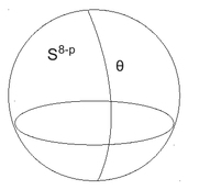
Figure 6: Constant embedding

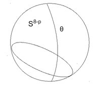
Figure 7: Embeddings $\theta=\theta(\psi)$.

it would have also resulted to a similarly complicated differential equation. The two different embeddings in that case are depicted in Figures 6 and 7 above.

For non-constant embeddings $\theta=\theta(\psi)$ in the underformed case, it is obviously possible to rotate the north pole in a way to obtain the first configuration. In practice, this is done by performing an $SO(6)$ transformation. In the $\sigma$-deformed case it is not obvious what the corresponding transformation would be, given that the isometry group has been reduced. The deformed sphere has the same Euler characteristic with the undeformed one, so that their topology is the same. It makes sense, then, to assume that such a transformation exists, although we were not able to find it.

4 Turning on temperature

It is natural to extend the discussion to asymptotically AdS spacetimes, which are relevant to a holographic approach to dimers in condensed matter systems, as pursued in [8]. We will briefly discuss the near horizon geometry of black D3-branes in such a way that the submanifold $\mathbb{S}^{1}\times\mathbb{S}^{3}$ of $\mathbb{S}^{5}$ appears explicitly. The metric of the background is

$$ds^{2}=-f(r)dt^{2}+\frac{dr^{2}}{f(r)}+\frac{r^{2}}{R^{2}}d\vec{x}^{2}_{||}+R^{2}(d\theta^{2}+\cos^{2}\theta~{}d\Omega_{1}^{2}+\sin^{2}\theta~{}d\Omega_{3}^{2})\ ,\quad f(r)=\frac{r^{4}-\mu^{4}}{R^{2}r^{2}},$$ (39)

and the RR-potential changes also accordingly. The Hawking temperature is simply proportional to the parameter $\mu$. We consider a D5-brane probe with the same embedding coordinates as before, i.e. $\vec{x}_{||}={\rm const.}$ and $\theta=\theta(r)$. It is a straightforward task to show that the minima of the particular configuration remain the same as with the zero temperature case, this being true for every $p$. This wouldn’t be the case for more general $r$-dependent solutions.

In order to ensure the stability of the configurations, one can consider small fluctuations around the minima. Let

$$\theta=\bar{\theta}+\xi,\qquad F_{tr}=\bar{F}_{tr}+\chi\ ,$$ (40)

where the bars denote the minima and $\chi=\partial_{t}\alpha_{r}-\partial_{r}\alpha_{t}$. It should be stressed out that this is consistent as long as one considers only the zero mode in the spherical harmonic expansion on the $\mathbb{S}^{5}$. In order to find the complete spectrum, one should also turn on fluctuations of the field strength in every possible direction (see also [13] for a prime example). However, here we are only interested in demonstrating perturbative stability at non-zero temperature, and for that, restricting to the zero-mode suffices. The effective Lagrangian for quadratic fluctuations is found to be

$$\mathcal{L} = \tfrac{1}{2}\sqrt{h}R^{4}T_{5}\cos\bar{\theta}\sin^{3}\bar{\theta}\frac{1}{\sqrt{1-\bar{F}^{2}_{tr}}}\left[R^{2}\left(f(r)^{-1}(\partial_{t}\xi)^{2}-f(r)(\partial_{r}\xi)^{2}\right)\right.$$ (42)

$$\qquad\qquad+\left.\frac{\chi^{2}}{1-\bar{F}^{2}_{tr}}+A\xi^{2}+B\chi\xi\right]\ .$$

The minima and the gauge field are given by

$$\sin\bar{\theta}=\sqrt{\frac{4}{3}\nu}\ ,\qquad\bar{F}_{tr}=\frac{9-16\nu}{\sqrt{81-96\nu}}\ ,$$ (43)

and we have defined the constants

$$A=4+\frac{36}{27-32\nu}\ ,\qquad B=\sqrt{81-96\nu\over 3\nu-4\nu^{2}}\ .$$ (44)

We obtain the equations of motion by varying $\chi$ and $\xi$. After combining them and concentrating on a Fourier mode of the form $\xi=e^{i\omega t}\Psi(r)$, we get

$${d\over dr}\left(f(r){d\Psi\over dr}\right)+\left({\omega^{2}\over f(r)}-{C\over 2R^{2}}\right)\Psi(r)=0\ ,\qquad C\equiv 24+\frac{72}{32\nu-27}\ ,$$ (45)

defined for $r\geqslant\mu$. We transform this into a Schrödinger equation for $\Psi$, by appropriately changing to a new variable $z=\int_{r}^{\infty}dr^{\prime}f^{-1}(r^{\prime})$, with $z\in[0,\infty)$ as $r\in(\infty,\mu]$. The associated potential, that can be written explicitly only in terms or $r$, is

$$V=\frac{C}{2}\frac{f(r)}{R^{2}}\ .$$ (46)

Substituting the value for $\theta$ in $C$ from (43) one sees that $C$ is non-negative. Hence the zero mode of the configuration is always positive. In fact, $C$ vanishes for the critical value $\nu={3/4}$. In conclusion, the configuration that we considered is stable. Similar arguments also hold for the other submanifolds and for the cases $p=0,1,2,4$ as well.

5 Application on holographic dimers

It is interesting to investigate how the results of the previous sections affect the holographic description of dimers. The main idea was pioneered in [8]. There, the authors considered lattices of D5-branes embedded in a D3 black brane background in order to model a finite temperature system. The chosen embedding is such that each probe brane wraps an $\mathbb{S}^{4}\subset\mathbb{S}^{5}$. By generalizing the arguments presented there, we will show in the present section that the less symmetric embeddings we found in section 2 are more favorable in the aforementioned context.

The metric of the background under consideration is (39), alongside with the parametrization (5) for the compact manifold restricted to the case with $p=3$. Hence the embedded branes wrap an $AdS_{2}$ space times a four dimensional submanifold. The free energy of the single D5-brane (or an anti-D5-brane) is computed by integrating the on-shell action [14]. In order to do this, one performs a Wick rotation to the Euclidean metric where time is identified as a periodic variable, which is the temperature. The free energy of a single D5-brane that goes straight down to the D3-horizon is given then by

$$F_{\textrm{D5}}=-\lambda\mu NT_{f}\mathcal{E}_{3,q}\ .$$ (47)

We observe that the result is proportional to the energies that we computed in section 2. The computation is very similar to that performed for the $q=1$ case in [14] so that we omit the details.

As in [8], we will consider a lattice of D5- and an anti-D5-brane pairs. Each pair is essentially constituted by a D5-brane which dives into the bulk and returns with an opposite orientation, thus regarded as an anti-D5-brane. There exist two configurations then, for each pair, depending on the value of the temperature. In the disconnected configuration the D5- and the anti-D5-brane are separated and do not interact. The total free energy of the pair is just the sum of the individual free energies, that is simply equal to

$$F_{\textrm{disconnected}}=2F_{\textrm{D5}}\ .$$ (48)

As will become transparent below, this configuration dominates at high temperature.

In the second configuration in which the D5- and the anti-D5-brane are connected with each other, the two membranes are separated by $\Delta x$ and are located at $r=\infty$ with $\vec{x}=(\pm\frac{\Delta x}{2},0,0)$. One considers then embeddings with $\theta(r)=\theta_{\nu}$ and $x=x(r)$. The turning point of the D5-brane is computed by $dr/dx^{\prime}=0$ and has the same form for a generic wrapping. We scale the turning point by the temperature and we define the dimensionless parameter $\displaystyle z_{0}\equiv\frac{r_{\textrm{turn}}}{\mu}$. The turning point is associated with the spacing between the branes and the temperature by the following relation

$$\frac{\mu}{R^{2}}\Delta x=\left[2(z_{0}^{4}-1)^{1/2}\int_{z_{0}}^{\infty}dz\sqrt{\frac{1}{(z^{4}-1)(z^{4}-z_{0}^{4})}}\right]\ .$$ (49)

Noting the similarity with the holographic computation of the binding energy of a quark-antiquark pair we mentioned above, we perform the integration obtaining [17]

$$\frac{\mu}{R^{2}}\Delta x=\frac{1}{2}B(3/4,1/2)\frac{\sqrt{z_{0}^{4}-1}}{z_{0}^{3}}~{}{}_{2}F_{1}\left(\frac{1}{2},\frac{3}{4},\frac{5}{4};\frac{1}{z_{0}^{4}}\right)\ .$$ (50)

As seen in Figure 8, for fixed lattice spacing $\Delta x$, a solution of this type exists only for low enough temperatures. For higher temperatures, the disconnected configuration is the only available solution. The critical temperature beyond which the latter dominates is not however given by the maximum value of the temperature, since the disconnected configuration already acquires a lower free energy at a lower temperature. To see that we compute the free energy of the connected configuration which is found to be

$$F_{\textrm{connected}} = 2\lambda\mu NT_{f}\mathcal{E}_{3,q}\left[-z_{0}+\int_{z_{0}}^{\infty}dz\left(\sqrt{\frac{z^{4}-1}{z^{4}-z_{0}^{4}}}-1\right)\right]$$ (51)

$$\equiv 2\lambda\mu NT_{f}\mathcal{E}_{3,q}\tilde{F}_{\textrm{connected}}\ ,$$ (52)

where we have defined the function

$$\tilde{F}_{\textrm{connected}}=\frac{z_{0}}{4}B\left(-1/4,1/2\right){}_{2}F_{1}\left(-\frac{1}{2},-\frac{1}{4},\frac{1}{4};\frac{1}{z_{0}^{4}}\right)\ ,$$ (53)

and we have computed the integral. This measures the deviation of the free energy from that of the disconnected configuration. To proceed with the analysis we note from Figure 8 that for the same temperature there exist two values of $z_{0}$. This mutlivalueness is also manifest in the plot of the free energy for the connected configuration in Figure 10. Based on the experience with a general analysis for the quark-anti-quark binding energy performed in [18], we expect that a similar analysis here will indicate that the upper branch is unstable under small perturbations, so that we disregard it completely. Note also that in Figures 8, 9 and 10 the black, red and blue colored branches correspond to the unstable, meta-stable and stable branches, respectively.

Next, we compare the free energy of the connected configuration as a function of $z_{0}$ with that of the disconnected configuration. We see from Figure 9 that for large values of $z_{0}$, equivalently for small temperatures, the connected configuration is more favorable. There exist a critical value of $z_{0}$, numerically equal to $z_{0,c}\simeq 1.52$,

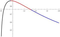
Figure 8: $\frac{\mu\Delta x}{R^{2}}$ as a function of $z_{0}$.

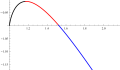
Figure 9: $\tilde{F}_{\textrm{connected}}$ as a function of $z_{0}$.

below which the disconnected configuration is favorable. Therefore, there exists a critical temperature at which the system undergoes a phase transition. This phase transition is of first order, since the first derivative possesses a discontinuity at the critical value $z_{0,c}$.

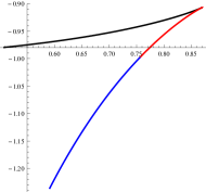
Figure 10: $\tilde{F}_{\textrm{connected}}$ as a function of $\frac{\mu\Delta x}{R^{2}}$.

Eventually, in order to make contact with the results of section 2, we first observe that (53) is the same for all wrappings. Thus the only difference in (52) for different wrappings origins simply from the constant factor in front, which is essentially the energy of the wrapping. Since $\tilde{F}_{\textrm{connected}}$ is always negative then, the wrapping with the heighest energy density, which is less symmetric, has the minimal free energy, becoming more favorable in this context. By considering lattices of pairs then one constructs dimers in a holographic way, along the lines presented in [8].

6 Concluding remarks

We classified and energetically compared all possible cases, with a single embedding angular coordinate, in which a D(8-p) brane can wrap $AdS_{2}$ times a submanifold of $\mathbb{S}^{8-p}$ in a Dp-brane background, thus producing a pointlike defect. We worked out the details in all different cases that arise, performing also comparisons between them. We examined similar constructions in the presence of temperature and in $\beta$-deformed backgrounds. We demonstrated stability by a small fluctuation analysis around the minima.

It would be interesting to investigate and search for running solutions of the embedding coordinate, i.e. $\theta=\theta(r)$. This involves the classical equation of motion for the Hamiltonian (20). This is a highly non-linear equation but it should be possible to analyze it numerically. Of particular interest would be solutions connecting minima corresponding to different values of $n$, especially when they correspond to the same energy.

Moreover, it would be very useful to extend our results beyond the probe approximation, by considering the backreaction of the probe branes on the background. This is significant when their number is comparable to the color number. In addition, these backreaction effects would also influence the dimerization analysis presented here, in case where many branes are located at each lattice site.

Acknowledgements

We would like to thank K. Siampos and D. Zoakos for useful discussions on the subject. N.K. acknowledges financial support provided by the Research Committee of the University of Patras via a K. Karatheodori fellowship under contract number C. 915.

References

• [1] C.ย Bachas, M.ย R.ย Douglas and C.ย Schweigert, Flux stabilization of D-branes, JHEP 0005 (2000) 048, arXiv:hep-th/0003037.
• [2] C.ย Bachas and M.ย Petropoulos, Anti-de Sitter D-branes, JHEP 0102 (2001) 025, hep-th/0012234.
• [3] J.ย Pawelczyk and S.-J.ย Rey, Ramond-Ramond flux stabilization of D-branes, Phys.Lett. B493 (2000) 395-401, hep-th/0007154.
• [4] J.M.ย Camino, A.ย Paredes and A.V.ย Ramallo, Stable wrapped branes, JHEP 0105 (2001) 011, hep-th/0104082.
• [5] A.ย Karch and L.ย Randall, Open and closed string interpretation of SUSY CFTโ€™s on branes with boundaries, JHEP 0106 (2001) 063, hep-th/0105132.
• [6] O.ย DeWolfe, D.ย Z.ย Freedman and H.ย Ooguri, Holography and defect conformal field theories, Phys. Rev. D66 (2002) 025009, hep-th/0111135.
• [7] K.ย Skenderis and M.ย Taylor, Branes in AdS and p-p wave space-times, JHEP 0206 (2002) 025, hep-th/0204054.
• [8] S.ย Kachru, A.ย Karch and S.ย Yaida, Holographic Lattices, Dimers, and Glasses, Phys.ย Rev.ย  D81 (2010) 026007, hep-th/0909.2639.
• [9] O.ย Lunin and J.M.ย Maldacena, Deforming field theories with $U(1)\times U(1)$ global symmetry and their gravity duals, JHEP 0505 (2005) 033, hep-th/0502086.
• [10] G.T.ย Horowitz and A.ย Strominger, Black strings and P-branes, Nucl. Phys. B360 (1991) 197-209.
• [11] C.N.ย Pope, Eigenfunctions and spinstructures in $CP^{2}$, Phys. Lett. B97 (1980) 417.
• [12] B.E.ย W.ย Nilsson and C.N.ย Pope, Hopf Fibration Of Eleven-dimensional Supergravity, Class. Quant. Grav. 1 (1984) 499.
• [13] M.ย Kruczenski, D.ย Mateos, R.C.ย Myers and D.J.ย Winters, Meson spectroscopy in AdS / CFT with flavor, JHEP 0307 (2003) 049, hep-th/0304032.
• [14] S.ย Yamaguchi, Wilson loops of anti-symmetric representation and D5-branes, JHEP 0605 (2006) 037, hep-th/0603208.
• [15] S.-J.ย Rey, S.ย Theisen, J.-T.ย Yee, Wilson-Polyakov loop at finite temperature in large N gauge theory and anti-de Sitter supergravity, Nucl. Phys. B527 (1998) 171, hep-th/9803135.
• [16] A.ย Brandhuber, N.ย Itzhaki, J.ย Sonnenschein, S.ย Yankielowicz, Wilson loops in the large N limit at finite temperature, Phys. Lett. B434 (1998) 36, [hep-th/9803137.
• [17] A.ย Brandhuber and K.ย Sfetsos, Wilson loops from multicenter and rotating branes, mass gaps and phase structure in gauge theories, Adv. Theor. Math.ย Phys. 3 (1999) 851, arXiv:hep-th/9906201.
• [18] S.ย D.ย Avramis, K.ย Sfetsos, K.ย Siampos, Stability of strings dual to flux tubes between static quarks in $N=4$ SYM, Nucl. Phys. B769 (2007) 44-78, hep-th/0612139.