ICRR-REPORT-586-2011-3

UCI-TR-2011-04

R-symmetry Matching In SUSY Breaking Models

Jessica Goodman^a, Masahiro Ibe^b,
Yuri Shirman^a, and Felix Yu^a

^a Department of Physics, University of California, Irvine, CA 92697.

^b Institute for Cosmic Ray Research, University of Tokyo, Chiba 277-8582, Japan

j.goodman@uci.edu, ibe@icrr.u-tokyo.ac.jp,
yshirman@uci.edu, felixy@uci.edu

Low energy descriptions of metastable supersymmetry breaking models often possess an accidental R-symmetry. Viable phenomenological applications of this class of models require R-symmetry to be broken in the ground state. This can be achieved in O’Raifeartaigh-like models where some of the chiral superfields carry negative R-charges. In this paper we consider UV completions of this class of models and formulate necessary conditions that they must satisfy. We show that the R-symmetry of the IR description can be traced to an anomalous or anomaly-free R-symmetry of the UV theory and discuss several representative examples.

PACS codes: 11.30.Pb, 11.30.Qc, 12.60.Jv

1 Introduction

Supersymmetry has been extensively explored as one of the most plausible extensions of the Standard Model at the TeV scale. One of its most attractive features is the potential to solve the gauge hierarchy problem. Models with softly broken supersymmetry guarantee that the electroweak scale is radiatively stable, thus providing a solution for the technical naturalness problem. In addition, if supersymmetry is broken dynamically, such breaking is necessarily non-perturbative and the SUSY breaking scale is naturally small compared to the fundamental scale of the theory (such as the Grand Unification scale or the Planck scale). Understanding of the dynamical supersymmetry breaking is especially important in scenarios with gauge mediated supersymmetry breaking (GMSB). Indeed, in GMSB models, supergravity contributions to the parameters of the low energy Lagrangian are negligible and studies of the full theory, including both the Standard Model and SUSY breaking sectors, may be under full theoretical control. Moreover, in models with extremely low SUSY breaking scales (of order tens or hundreds of TeV), many new particles or interactions may be experimentally accessible.

However, it is difficult to find DSB models with phenomenologically desirable features. Moreover, once the DSB sector is coupled to the Standard Model, the SUSY breaking vacuum generically survives only as a local minimum of the potential. This is acceptable as long as the lifetime of the metastable vacuum is sufficiently long. The model building prospects improved significantly when Intriligator, Seiberg, and Shih (ISS) [1] proposed to embrace metastability as a fundamental feature of the models. They showed that metastable, long-lived (and often calculable) non-supersymmetric vacua are generic in SUSY gauge theories. ISS models usually possess an accidental R-symmetry which is unbroken in the metastable vacuum. This poses a significant obstacle to constructing viable extensions of the Standard Model since an unbroken R-symmetry forbids gaugino masses. Several implementations of direct gauge mediation based on ISS models proposed in the literature [2, 3, 4] circumvent this difficulty by modifying the underlying theory so that R-symmetry is broken either explicitly or spontaneously. Nevertheless, it was argued in [5] that even then gaugino masses are numerically suppressed compared to sfermion masses. The phenomenology of low scale GMSB models with spontaneous and explicit R-symmetry breaking as well as the ability to discriminate these two classes was investigated in [6].

Motivated by these problems, Shih studied conditions for spontaneous R-symmetry breaking in O’Raifeartaigh-like models [7]. He found that the Coleman-Weinberg potential may result in simultaneous supersymmetry and R-symmetry breaking if the model contains chiral superfields with R-charges other than $0$ and $2$. This requirement implies that models must contain at least one chiral superfield with a negative R-charge. Although the O’Raifeartaigh description is often sufficient for phenomenological purposes, it is desirable to understand R-symmetry breaking dynamics in terms of a complete UV description. The requirement of negative R-charges suggests that searching for a UV description may be tricky. Indeed, the presence of negative R-charges allows one to write superpotential terms with negative exponents of the superfields. Such terms must be forbidden by the symmetries of the microscopic physics — otherwise they would necessarily be generated dynamically and destabilize the SUSY breaking minimum.

In this paper we will study general requirements for UV completions of O’Raifeartaigh-like models with perturbative R-symmetry breaking. We will show that in viable models the low energy R-symmetry arises as a linear combination of a (possibly anomalous) R-symmetry of the UV physics and an anomaly-free global symmetry. In the case of an anomalous R-symmetry, R-charges of all physical fields in the microscopic description will be anomalous. When the R-symmetry is anomaly-free, R-charges of the low energy fields arise due to contributions of the non-R global symmetry. In this case dangerous operators do not appear since the non-R global symmetry is respected by all the non-perturbative dynamics.

2 General properties of UV completions

We are interested in models of metastable SUSY breaking where some of the low energy degrees of freedom are composites of the microscopic physics . There exist several possibilities for the origin of the R-symmetry of the low energy physics:

• An R-symmetry of the low energy description arises from the non-anomalous R-symmetry of the microscopic physics. In this case, the R-symmetry is a symmetry of the Lagrangian at all scales. Many classic models of dynamical supersymmetry breaking belong to this class. They possess R-symmetries under which some superfields carry negative charges. Non-perturbative dynamics generates superpotential terms with negative powers of the superfields. Both SUSY and R-symmetry are broken due to the interplay between tree level and non-perturbative interactions while perturbative corrections are small. In Sec. 4.1, we will show that this class of models also contains theories where negative exponents of superfields do not appear in the dynamical superpotential and R-symmetry is broken by perturbative dynamics.

• An R-symmetry of the IR physics corresponds to an anomalous R-symmetry of the ultraviolet description. Since the R-symmetry is anomalous, it will necessarily be broken by non-perturbative dynamics. As we will show, the existence of the negative R-charges in the low energy description implies that the microscopic theory contains at least some elementary chiral superfields with negative R-charges. Thus, in general, it is possible that the superpotential terms containing fields with negative exponents will be generated by the non-perturbative dynamics. Such terms can never be negligible near the origin of the moduli space. In models with classical flat directions they tend to destabilize the SUSY breaking vacuum of the O’Raifeartaigh-like model. However, we will construct models where an anomalous R-symmetry is given by a linear combination of anomalous and anomaly-free symmetries (e.g. baryon number). While certain composites carry negative R-charge, they only show up in the dynamical superpotential in combination with fields carrying sufficiently large positive R-charge so that the dynamical superpotential does not contain superfields with negative exponents. As a result, the SUSY and R-symmetry breaking minimum of an O’Raifeartaigh model will survive as a local minimum of the UV completion. We will discuss the correspondence between an accidental R-symmetry of the effective low energy description and an anomalous R-symmetry of the microscopic theory in Secs. 4.2 and 4.3.

3 Anomalous R-symmetries and non-perturbative superpotentials in SQCD

Let us briefly review exact results from supersymmetric QCD. For our purposes it is convenient to follow the presentation of [10]. Consider an $SU(N)$ gauge theory with $F$ flavors in the fundamental representation. The quantum numbers of the fields under gauge and global symmetries are:

$$\begin{array}[]{c|c| c c c c c}&SU(N)_{\text{gauge}}&SU(F)_{L}&SU(F)_{R}&U(1)_{B}&U(1)_{A}&U(1)_{R}\\ \hline\cr Q&\Box&\Box&\mathbf{1}&1&1&0\\ \bar{Q}&\overline{\Box}&\mathbf{1}&\overline{\Box}&-1&1&0\\ \hline\cr\end{array}$$ (1)

Both the $U(1)_{A}$ and the $U(1)_{R}$ symmetries are anomalous. If we perform the corresponding symmetry transformation parametrized by an angle $\alpha$, each fermion transforming under representation $r$ and carrying charge $q_{r}$ under the anomalous symmetries will contribute a factor of $n_{r}\alpha F\tilde{F}$ to a shift in the Lagrangian, where $n_{r}$ is an anomaly coefficient given by

$$n_{r}=2q_{r}C(r)=\left\{\begin{array}[]{ll}q_{r}&r=\Box\text{ or }\overline{\Box}\\ 2Nq_{r}&r=\text{ adjoint}\ .\\ \end{array}\right.$$ (2)

This shift can be absorbed into a redefinition of the $\theta$-angle, $\theta\rightarrow\theta-\sum_{r}n_{r}\alpha$, thus formally restoring the symmetry. In SUSY gauge theories, the gauge coupling and the $\theta$-angle combine into a holomorphic background superfield $\tau$ given by

$$\tau=\frac{\theta}{2\pi}+\frac{4\pi i}{g^{2}}\ .$$ (3)

Thus quantum physics remains formally invariant under anomalous symmetries if the gauge function $\tau$ transforms non-linearly:

$$\tau\rightarrow\tau-\frac{\sum_{r}n_{r}\alpha}{2\pi}\,.$$ (4)

For example, in the case of an anomalous R-symmetry, as defined in Eq. (1), the fermions in the quark supermultiplets carry R-charge $-1$, while the R-charge of gauginos is $1$. Thus $\sum n_{r}=2(N-F)$. On the other hand, the renormalization group evolution of the gauge coupling allows us to associate $\tau$ with the dynamical scale of the theory using

$$\Lambda^{b_{0}}=M^{b_{0}}e^{2\pi i\tau(M)}\ ,$$ (5)

where $b_{0}=3N-F$ is a one loop beta function coefficient of SUSY QCD and $\tau(M)$ is a running coupling evaluated at the scale $M$. We see that non-linear transformations of $\tau$ under the R-symmetry correspond to linear transformations of $\Lambda^{b_{0}}$ with R-charge $2(N-F)$. If we now specialize to models with $F<N$, we can easily see that the function

$$W=\left(\frac{\Lambda^{b_{0}}}{\det Q\bar{Q}}\right)^{\frac{1}{N-F}}$$ (6)

has an R-charge of 2. Similar arguments lead to the conclusion that $W$ is invariant under $U(1)_{A}$ if $\Lambda^{b_{0}}$ carries charge $2F$ under $U(1)_{A}$. Indeed, the superpotential of Eq. (6) is the celebrated non-perturbative Affleck-Dine-Seiberg (ADS) superpotential (in the case $F=N-1$, the overall coefficient of this term can be evaluated by an explicit instanton calculation). Applying this formalism to O’Raifeartaigh-like models, we will be able to relate the R-symmetry of the IR description to anomalous or anomaly-free symmetries of the UV physics.

4 Metastable dynamical SUSY breaking with spontaneously broken R-symmetry

It is well known that O’Raifeartaigh models possess pseudoflat directions in the field space which can be parameterized by vacuum expecation values (vevs) of moduli fields with R-charge 2. Thus, at a generic point on the pseudomoduli space, R-symmetry is spontaneously broken. Perturbative corrections lift the pseudoflat direction and generically stabilize pseudomoduli at the origin so that R-symmetry is unbroken in the ground state. It was shown in [7] that O’Raifeartaigh models can be generalized to a class of models where the Coleman-Weinberg potential results in the existence of a local minimum of the potential with spontaneously broken R-symmetry (albeit the SUSY breaking minimum is only a local one). Here we will discuss several UV completions of models in this class and will show how the R-symmetry of the effective description arises from the symmetries of the microscopic theory.

For simplicity we will study $SU(N)$ SQCD with $F$ flavors. As we have seen in Sec. 3, the maximal global symmetry is $SU(F)_{L}\times SU(F)_{R}\times U(1)_{B}\times U(1)_{A}\times U(1)_{R}$, where $U(1)_{A}$ and $U(1)_{R}$ are anomalous. If we require that non-perturbative dynamics does not generate superpotential terms that are singular at the origin of the moduli space, we must have $F>N-1$. On the other hand, to simplify the discussion we will assume that there are no light gauge fields in the IR description which implies $F<N+2$.

In Sec. 4.1 we study a model with $F=N$ and explain how an accidental R-symmetry of the IR physics can arise from an anomaly-free R-symmetry of the UV theory. In Secs. 4.2 and 4.3, we consider the case with $F=N+1$ and identify the R-symmetry of the low energy physics with an anomalous R-symmetry of the UV completion.

4.1 A model with a non-anomalous R-symmetry

The simplest SUSY and R-symmetry breaking model, introduced in [7], has the superpotential

$$W=\lambda X(\mu^{2}-\phi_{1}\phi_{2})+m_{1}\phi_{1}\phi_{3}+\frac{m_{2}}{2}\phi_{2}^{2}\ .$$ (7)

The model possesses an R-symmetry with the charges of the chiral superfields given by

$$R(X)=2,\quad R(\phi_{1})=-1,\quad R(\phi_{2})=1,\quad R(\phi_{3})=3\ .$$ (8)

Our UV completion will be based on a perturbation of the ITIY model [11, 12] with an $SU(2)$ gauge group, 4 doublet chiral superfields $Q_{i}$ and 6 gauge singlet fields $S_{ij}$ transforming under gauge and global symmetries as

$$\begin{array}[]{c|c| c c }&SU(2)_{\text{gauge}}&SU(4)&U(1)_{R}\\[2.15277pt] \hline\cr&&&\\ Q&\Box&{\Box}&0\\ S&1&\hbox{\rule{0.6pt}{7.0pt}\hskip-0.6pt\rule{7.0pt}{0.6pt}\hskip-7.0pt\rule[7.0pt]{7.0pt}{0.6pt}}\rule[7.0pt]{0.6pt}{0.6pt}\hskip-0.6pt\rule{0.6pt}{7.0pt}\hskip-7.6pt\raisebox{7.0pt}{\hbox{\rule{0.6pt}{7.0pt}\hskip-0.6pt\rule{7.0pt}{0.6pt}\hskip-7.0pt\rule[7.0pt]{7.0pt}{0.6pt}}\rule[7.0pt]{0.6pt}{0.6pt}\hskip-0.6pt\rule{0.6pt}{7.0pt}}&2\\ \hline\cr&&&\end{array}$$ (9)

The classical superpotential is chosen to be

$$W=\sum\limits_{i,j=1,\ i<j}^{4}\lambda_{ij}S_{ij}Q_{i}Q_{j}+\frac{(Q_{3}Q_{4})^{2}}{\Lambda_{UV}}+\frac{m_{S}}{2}S_{34}^{2}\ .$$ (10)

The second two terms in Eq. (10) break the maximal anomaly-free global symmetry down to $SO(4)\times U(1)^{\prime}_{R}$, where the unbroken anomaly-free R^′-symmetry is a linear combination of the original R-symmetry and the $U(1)_{F}$ subgroup of $SU(4)$ generated by $T=\text{diag}(-1,-1,1,1)$. The R^′-symmetry charges are given by

$$\begin{split}&R^{\prime}(Q_{1})=R^{\prime}(Q_{2})=-\frac{1}{2}\ ,\quad R^{\prime}(Q_{3})=R^{\prime}(Q_{4})=\frac{1}{2}\ ,\\ &R^{\prime}(S_{12})=3\ ,\quad R^{\prime}(S_{34})=1\ ,\quad R^{\prime}(S_{1})=R^{\prime}(S_{2})=R^{\prime}(S_{3})=R^{\prime}(S_{4})=2\ .\end{split}$$ (11)

One of the important features of the ITIY model is the absence of classical flat directions involving quark superfields. A quick analysis of Eq. (10) shows that for generic choices of the tree-level parameters this remains true in the presence of our perturbation. Classical flat directions are reintroduced when $\lambda_{34}^{2}/(2m_{S})-1/\Lambda_{UV}=0$, leading to restoration of supersymmetry.

Let us show the correspondence between the models defined by Eqs. (7) and (10). The full superpotential of the perturbed ITIY model is

$$W=\chi(\text{ Pf }M-\Lambda^{4})+\sum_{ij}\lambda_{ij}S_{ij}M_{ij}+c\frac{M_{34}^{2}}{\Lambda_{UV}}+\frac{m_{S}}{2}S_{34}^{2}\ ,$$ (12)

where $\chi$ denotes the Lagrange multiplier which represents the quantum deformed moduli constraint. Our perturbation singles out two mesons, $M_{12}=(Q_{1}Q_{2})$ and $M_{34}=(Q_{3}Q_{4})$, and their associated singlets. We will use the unbroken $SO(4)$ symmetry to denote the remaining mesons and singlets as $M_{a}$ and $S_{a}$, $a=1,\ldots 4$, respectively. Using the quantum constraint, we can integrate out one of the mesons, say $M_{1}$,

$$M_{1}=\left(\Lambda^{4}-\sum\limits_{a=2}^{4}M_{a}^{2}-2M_{12}M_{34}\right)^{1/2}\simeq\Lambda^{2}-\sum\limits_{a=2}^{4}\frac{M_{a}^{2}}{2\Lambda^{2}}-\frac{M_{12}M_{34}}{\Lambda^{2}}+\ldots$$ (13)

where the dots represent higher order terms in the expansion. The superpotential becomes

$$\begin{array}[]{ccl}W&=&\lambda_{1}S_{1}\left(\Lambda^{2}-\sum\limits_{a}\frac{M_{a}^{2}}{2\Lambda^{2}}-\frac{M_{12}M_{34}}{\Lambda^{2}}\right)\\ &+&\sum\limits_{a}\lambda_{a}S_{a}M_{a}+\lambda_{12}S_{12}M_{12}+\lambda_{34}S_{34}M_{34}+c\frac{M_{34}^{2}}{\Lambda_{UV}}+\frac{m_{S}}{2}S_{34}^{2}\ .\end{array}$$ (14)

Once we integrate out the massive fields, $M_{a}$, $S_{a}$, and $S_{34}$, the correspondence between UV and IR descriptions becomes obvious:

$$X\sim S_{1},\quad\phi_{1}\sim M_{12}/\Lambda,\quad\phi_{2}\sim M_{34}/\Lambda,\quad\phi_{3}\sim S_{12}\ .$$ (15)

Thus the pseudomoduli spaces of the two models are identical.

It is important to note that relation Eq. (15) constrains the coupling constants and masses of fields in the low energy effective description according to

$$\mu\sim\Lambda,\quad\lambda\sim\lambda_{1},\quad m_{1}\sim\lambda_{12}\Lambda,\quad m_{2}\sim\left(\frac{1}{\Lambda_{UV}}-\frac{\lambda_{34}^{2}}{2m_{S}}\right)\Lambda^{2}\ .$$ (16)

In the model from Eq. (7), SUSY is restored when $m_{2}$ is massless. From the point of view of the microscopic description, this happens precisely when UV parameters are chosen so that the classical flat direction is reintroduced. On the other hand, for a generic choice of the parameters, the local SUSY breaking minimum exists and for a range of parameters, R-symmetry is broken in this vacuum (see Fig. 1).

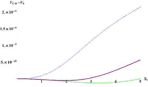
Figure 1: [color online]. Relative Coleman-Weinberg potential as a function of pseudomodulus $S_{1}$ for the model in Eq. (14) where $\Lambda=1$, $\Lambda_{UV}=10$, $\lambda_{1}=0.02$, $\lambda_{a}=1$, $\lambda_{12}=0.03$, $\lambda_{34}=0.03$, $m_{S}=1$, and $c$ varied from 0.2 (blue, dotted, top) to 0.6 (purple, solid, middle) to 1.0 (green, dashed, bottom).

The model we discussed here clearly exemplifies the importance of the UV completion, which possesses a larger set of anomaly-free global symmetries. Indeed, while superpotential terms with negative superfield exponents are allowed by all of the symmetries of the model of Eq. (7), such terms are forbidden by additional symmetries present in the UV completion of Eq. (10). In particular, the R-symmetry of the low energy physics is a linear combination of the $U(1)_{R}$ and vector-like $U(1)_{F}$ symmetries. In fact, it is $U(1)_{F}$ which is responsible for the appearance of composites with negative R-charges. At the same time, dynamical terms in the superpotential must be invariant under all anomaly-free global symmetries, thus preventing the appearance of the terms with negative exponents of the superfields.

4.2 A model with an anomalous R-symmetry

We have seen in the previous section that global symmetries of the UV physics play an important role in understanding of the IR dynamics of O’Raifeartaigh-like models. Therefore, we will consider a generalization of the model from Eq. (7) in the form

$$W=\lambda\phi_{i}X^{ij}\tilde{\phi}_{j}-\mu^{2}\phi_{1}+\frac{1}{2}m\text{ Tr }X^{2}+n\tilde{\phi}_{i}S^{i}\ ,$$ (17)

where $i,j=1,\ldots F,$ are flavor indices, $\mu$, $m$, and $n$ are mass parameters, and $\lambda$ is a coupling constant. The model possesses a large global symmetry, including an R-symmetry under which chiral superfields carry the following charges :

$$R_{\phi}=2,\quad R_{\tilde{\phi}}=-1,\quad R_{X}=1,\quad R_{S}=3\ .$$ (18)

For a UV completion, we will consider $SU(N)$ theory with $F=N+1$ flavors and map $\phi_{i}$, $\tilde{\phi}_{i}$ and $X_{ij}$ to baryons, anti-baryons and mesons of the microscopic description, respectively, while $S_{i}$ remain elementary:

$$\phi_{i}\sim B_{i}\ ,\quad\tilde{\phi}_{i}\sim\overline{B}_{i}\ ,\quad X_{ij}\sim M_{ij}\ .$$ (19)

In the absence of the superpotential, the global symmetry is $SU(F)_{L}\times SU(F)_{R}\times U(1)_{B}\times U(1)_{A}\times U(1)_{R}$. Charges of the matter fields, gauge invariant composites, and the dynamical scale $\Lambda$ are given by

$$\begin{array}[]{c|c| c c c c c}&SU(N)_{\text{gauge}}&SU(N+1)_{L}&SU(N+1)_{R}&U(1)_{B}&U(1)_{A}&U(1)_{R}\\[2.15277pt] \hline\cr&&&&&&\\ Q&\Box&{\Box}&1&\frac{1}{N}&\frac{1}{N}&0\\ \bar{Q}&\overline{\Box}&1&\overline{\Box}&-\frac{1}{N}&\frac{1}{N}&0\\ S&1&1&\overline{\Box}&1&-1&2\\ \hline\cr&&&&&&\\ \Lambda^{2N-1}&&&&&\frac{2(N+1)}{N}&-2\\ \hline\cr&&&&&&\\ B=Q^{N}&1&\overline{\Box}&1&1&1&0\\ \overline{B}=\overline{Q}^{N}&1&1&\Box&-1&1&0\\ M=Q\bar{Q}&1&\Box&\overline{\Box}&0&\frac{2}{N}&0\\ \hline\cr\end{array}$$ (20)

To analyze the model from the microscopic point of view, we need to choose a tree level superpotential that matches Eq. (17) as closely as possible. It is easy to check that the superpotential Eq. (17) does not possess any R-symmetry when written in terms of the elementary fields. An R-symmetry may appear if the superpotential depends on the dynamical scale $\Lambda$ which transforms under anomalous symmetries. Therefore, at least some terms in Eq. (17) must be generated dynamically. Indeed, it is well known [13, 14] that $\phi X\tilde{\phi}\sim BM\bar{B}/\Lambda^{2N-1}$ is generated non-perturbatively. Let us then restrict our attention to the remaining three terms in Eq. (17). If we require that these terms correspond to the tree level superpotential of the microscopic description, we find an anomalous R-symmetry given by

$$U(1)^{\prime}_{R}=U(1)_{R}+\frac{N}{2}U(1)_{A}+(2-\frac{N}{2})U(1)_{B}\ .$$ (21)

The full dynamical superpotential is

$$W=\lambda\frac{B_{i}M^{ij}\bar{B}_{j}-\det M}{\Lambda^{2N-1}}+c_{B}\frac{B_{1}}{\Lambda_{UV}^{N-3}}+c_{M}\frac{\text{ Tr }M^{2}}{\Lambda_{UV}}+c_{\bar{B}}\frac{\bar{B}_{i}S^{i}}{\Lambda_{UV}^{N-2}}\ ,$$ (22)

where the dimensionless coefficients $c_{B}$, $c_{M}$, and $c_{\bar{B}}$ are of $\mathcal{O}(1)$ in the absence of fine-tuning (we will see shortly that in this model one must choose $c_{B}\ll 1$). This superpotential is invariant under Eq. (21) once the transformation properties of $\Lambda$ are taken into account. An additional term, $\det M$, appearing in Eq. (22) remains irrelevant in the IR and decouples from low energy physics.

Since the existence of the R-symmetry in the UV description required an addition of the spurion $\Lambda^{2N-1}$, the matching of R-charges is not completely trivial. Charges of the tree-level terms $B_{1}$ and $\text{Tr }M^{2}$ must match directly between the UV and IR. Comparing the non-perturbative term to its counterpart in the IR superpotential, we see that the charge of $\bar{B}/\Lambda^{2N-1}$ matches the charge of $\tilde{\phi}$. This, in turn, determines the matching between UV and IR charges of the gauge singlet fields. The full set of relations between the R-charges is

$$R_{\phi}=R_{B}\ ,\quad R_{X}=R_{M}\ ,R_{\tilde{\phi}}=R_{\bar{B}}-R_{\Lambda^{2N-1}}\ ,\quad R_{S_{IR}}=R_{S_{UV}}+R_{\Lambda^{2N-1}}\ .$$ (23)

It is important to note that in our construction all the superfields of the microscopic theory have positive R-charges. Negative R-charges of the low energy effective description are due to the contribution of the anomaly through the spurion $\Lambda^{2N-1}$. This guarantees that all terms generated by non-perturbative dynamics are regular at the origin of the moduli space.

To study the Coleman-Weinberg potential, we first neglect the non-renormalizable term $\det{M}$ in Eq. (22) and thus restrict our attention to the superpotential Eq. (17). We also note that the parameters of the low energy model are related to those of the microscopic description according to

$$\mu^{2}=c_{B}\left(\frac{\Lambda}{\Lambda_{UV}}\right)^{N-3}\Lambda^{2}\ ,\quad\frac{m}{2}=c_{M}\left(\frac{\Lambda}{\Lambda_{UV}}\right)\Lambda\ ,\quad n=c_{\bar{B}}\left(\frac{\Lambda}{\Lambda_{UV}}\right)^{N-2}\Lambda\ ,$$ (24)

and $\lambda\sim\mathcal{O}(1)$. Otherwise, our analysis closely follows that of [7] and arrives at the same conclusions. It is easy to see that at tree level the model possesses a flat direction in the field space along which the energy is non-vanishing, with scalar potential $V_{min}=\mu^{4}$. This direction is parametrized by

$$\tilde{\phi_{i}}=S_{i}=0\ ,$$ (25)

$$X_{ji}=0\ ,$$

$$\text{ and }\phi_{i}\text{ arbitrary. }$$

There also exists a runaway direction along which SUSY is restored. Up to global symmetry transformations it is given by:

$$\phi_{1}=-\left(\frac{mn^{2}S_{1}^{2}}{\lambda^{2}\mu^{2}}\right)^{1/3},~{}~{}~{}~{}~{}X_{11}=\left(\frac{\mu^{2}nS_{1}}{\lambda m}\right)^{1/3},~{}~{}~{}~{}~{}\tilde{\phi}_{1}=\left(\frac{\mu^{4}m}{\lambda^{2}nS_{1}}\right)^{1/3},$$ (26)

with $\phi_{i}$, $\tilde{\phi}_{i}$, and $X_{ii}$ with $i\neq 1$ given by Eq. (25). Using global symmetry transformations, we can rotate any $\phi_{i}$ vev into $\phi_{1}$ and $\phi_{2}$. Assuming that $\langle\phi_{2}\rangle=0$, the superpotential for $\phi_{1}$ is similar to the R-symmetry breaking model discussed in [7], where it was shown that a metastable minimum may exist near the origin of the moduli space if (in our notation)

$$\begin{split}\frac{\lambda^{2}\mu^{4}}{m^{2}n^{2}}&<1\\ \frac{\lambda^{2}\mu^{4}-m^{2}n^{2}}{2m\lambda^{2}\mu^{2}}<\langle\phi_{1}\rangle&<\frac{m^{2}n^{2}-\lambda^{2}\mu^{4}}{2m\lambda^{2}\mu^{2}}\ .\end{split}$$ (27)

In terms of the parameters of the microscopic theory, these relations imply that $c_{B}\ll 1$. We now calculate the one loop correction to the potential to determine the mass of the pseudomoduli fields. A numerical calculation with arbitrary $\phi_{1}$ and $\phi_{2}$ shows a minimum of the Coleman-Weinberg potential at $\phi_{2}=0$. Thus, we expand the potential around the $\phi_{2}=0$ in order to obtain an analytic expression for the mass of $\phi_{1}$. We find, in agreement with [7],

$$m_{\phi_{1}}^{2}=-\frac{\lambda^{2}\mu^{4}}{8\pi^{2}}\frac{-3m^{4}+2m^{2}n^{2}+n^{4}+2m^{2}(m^{2}+3n^{2})\log(\frac{m}{n})}{(m^{2}-n^{2})^{3}}+Nf(\mu^{2},\lambda,m,n),$$ (28)

where $f(\mu^{2},\lambda,m,n)$ is strictly positive. For an appropriate choice of parameters, the pseudomodulus obtains a non-zero vacuum expectation value thus breaking the R-symmetry. In Fig. 2, we show the Coleman-Weinberg potential for a few different parameter choices, demonstrating that for a suitable choice of input UV parameters, we can drive the pseudomodulus $\phi_{1}$ to attain nonzero vev and break $R$-symmetry.

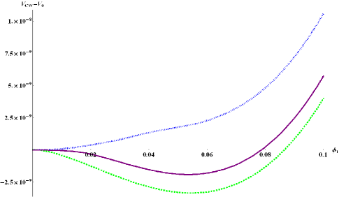
Figure 2: [color online]. Relative Coleman-Weinberg potential as a function of pseudomodulus $B_{1}$ for Eq. (22) with $\Lambda=1$, $\Lambda_{UV}=10$, $N=4$, $\lambda=1$, $c_{B}=0.1$, $c_{M}=4.0$, and $c_{\bar{B}}$ varied from 1.5 (green, dashed, bottom) to 2.5 (purple, solid, middle) to 3.5 (blue, dotted, top).

We now turn our attention to the $\det M$ term present in the full dynamical superpotential. We note that it does not destabilize the location of the SUSY breaking vacuum since it vanishes in the vicinity of this minimum. Interestingly, $\det M$ is also vanishing along the runaway direction. This seems to imply that the runaway behavior persists in the full theory. On the other hand, the analysis of the tree-level superpotential shows that the only classical flat directions are associated with gauge singlets $S_{i}$. Thus there can be no runaways with large vevs for composites $M$, $B$, and $\bar{B}$. This apparent contradiction is resolved by a careful examination of the vevs in Eq. (26) to $\Lambda$ and the UV cutoff $\Lambda_{UV}$. In terms of composites of the microscopic theory, we find

$$\begin{split}\frac{B_{1}}{\Lambda^{N}}\sim\left(\frac{\Lambda}{\Lambda_{UV}}\right)^{\frac{N-2}{3}}\left(\frac{S}{\Lambda_{UV}}\right)^{\frac{2}{3}}\lower 2.15277pt\hbox{$\>\buildrel<\over{\sim}\>$}\left(\frac{\Lambda}{\Lambda_{UV}}\right)^{\frac{N-2}{3}}\\ \frac{M}{\Lambda^{2}}\sim\left(\frac{\Lambda}{\Lambda_{UV}}\right)^{\frac{2N-7}{3}}\left(\frac{S}{\Lambda_{UV}}\right)^{\frac{1}{3}}\lower 2.15277pt\hbox{$\>\buildrel<\over{\sim}\>$}\left(\frac{\Lambda}{\Lambda_{UV}}\right)^{\frac{2N-7}{3}}\ ,\\ \end{split}$$ (29)

where we chose the maximal value for $c_{B}$ and in the second inequality on each line we used the fact that even in terms of elementary quarks our theory is only an effective description valid below $\Lambda_{UV}$. We conclude that along the runaway direction this effective theory breaks down before the perturbative regime of the $SU(N)$ gauge dynamics is reached. Thus the reliable determination of the global supersymmetric minimum of the model requires one to specify the origin of the non-renormalizable terms in Eq. (22).

4.3 An anomalous R-symmetry in a deformation of an ISS model

It is instructive to consider another effective model given by the superpotential

$$W=\lambda\phi_{i}X^{ij}\tilde{\phi}_{j}-\mu^{2}\text{ Tr }X+\frac{1}{2}m\phi_{i}^{2}+n\tilde{\phi}_{i}S^{i}\ ,$$ (30)

where $i,j=1,\ldots F$ are flavor indices as before. The R-symmetry charges of the chiral superfields are given by 

$$R_{X}=2\ ,\quad R_{\phi}=1\ ,\quad R_{\tilde{\phi}}=-1\ ,\quad R_{S}=3\ .$$ (31)

It is easy to see that once again the model possesses both runaway and pseudoflat directions in the field space. The pseudoflat direction is parametrized by

$$\begin{split}\phi_{i}=\tilde{\phi}_{i}=S_{i}=0\\ X_{ij}\text{ arbitrary}\ ,\end{split}$$ (32)

and the energy along this direction is $V_{min}=(N+1)\mu^{4}$, where $F=N+1$. Most of the $X$ fields are perturbatively stabilized at the origin. On the other hand, the Coleman-Weinberg potential for $X_{11}$ is the same as the potential for the pseudomodulus in the model of [7]. In particular for $r\equiv m/n\gtrsim 2.11$, the mass of $X_{11}$ is negative and a local minimum with spontaneously broken R-symmetry exists.

The runaway direction is given by

$$X_{11}=-\left(\frac{mn^{2}S_{1}^{2}}{\lambda^{2}\mu^{2}}\right)^{1/3}\,,~{}~{}~{}~{}~{}\phi_{1}=\left(\frac{\mu^{2}nS_{1}}{\lambda m}\right)^{1/3}\,,~{}~{}~{}~{}~{}\tilde{\phi}_{1}=\left(\frac{\mu^{4}m}{\lambda^{2}nS_{1}}\right)^{1/3}\ ,$$ (33)

and in the limit $S_{1}\rightarrow\infty$, the vacuum energy is lowered to $V_{min}=N\mu^{4}$. Once again, the remaining $X$ fields are stabilized at the origin by perturbative corrections.

We now turn to the analysis of the UV completion of this model. Once again we will look for a microscopic description in terms of a deformation of an s-confining SQCD. The association between gauge invariant composites of the microscopic description and the fields of the low energy model is the same as before, see Eq. (19). The full non-perturbative superpotential of the UV complete description is given by

$$W=\lambda\frac{B_{i}M^{ij}\bar{B}_{j}-\det M}{\Lambda^{2N-1}}+m_{Q}\text{ Tr }M+d_{B}\frac{B_{i}^{2}}{\Lambda_{UV}^{2N-3}}+d_{\bar{B}}\frac{\bar{B}_{i}S^{i}}{\Lambda_{UV}^{N-2}}\ .$$ (34)

In this case, the parameters of the UV and IR descriptions are related by

$$\mu^{2}=m_{Q}\Lambda\ ,\quad\frac{m}{2}=d_{B}\left(\frac{\Lambda}{\Lambda_{UV}}\right)^{2N-3}\Lambda\ ,\quad n=d_{\bar{B}}\left(\frac{\Lambda}{\Lambda_{UV}}\right)^{N-2}\Lambda\ ,$$ (35)

and $\lambda\sim\mathcal{O}(1)$. Requiring that R-symmetry is spontaneously broken we find

$$r=2\frac{d_{B}}{d_{\bar{B}}}\left(\frac{\Lambda}{\Lambda_{UV}}\right)^{N-1}\gtrsim 2.11\,.$$ (36)

Thus R-symmetry breaking requires a mild hierarchy between parameters of tree level superpotential $d_{B}>d_{\bar{B}}$. The Coleman-Weinberg potential for several choices of the parameters is shown in Fig. 3.

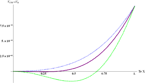
Figure 3: [color online]. Relative Coleman-Weinberg potential as a function of pseudomodulus Tr $X$ for the model in Eq. (34) where $\Lambda=1$, $\Lambda_{UV}=10$, $N=2$, $\lambda=1$, $m_{Q}=0.1$, $d_{B}=8$, and $d_{\bar{B}}$ varied from 0.50 (green, dashed, bottom) to 0.70 (purple, solid, middle) to 0.90 (blue, dotted, top).

The analysis of the symmetries in this model is analogous to that in Sec. 4.2. Tree level terms in the superpotential are invariant under an anomalous $U(1)_{R}$ symmetry given by

$$U(1)^{\prime}_{R}=U(1)_{R}+NU(1)_{A}-(N-1)U(1)_{B}\ .$$ (37)

Furthermore, assigning the charge $2N$ to the dynamical scale $\Lambda^{2N-1}$ makes the full non-perturbative potential invariant under this symmetry. The R-symmetry matching between the UV and IR is again given by  Eq. (23). Once again, there are no fields with negative R-charges in the microscopic description.

We conclude this section by discussing the restoration of SUSY in the microscopic description. Recall that there are no supersymmetric ground states in the low energy description given by Eq. (30). Moreover, $\det M\sim\det X$ vanishes along the non-supersymmetric runaway Eq. (33). However, the presence of this non-perturbatively generated term leads to the appearance of supersymmetric vacua elsewhere.

5 Conclusions

O’Raifeartaigh-like models with spontaneously broken R-symmetry require that some of the IR degrees of freedom carry negative R-charges. Therefore symmetries of the low energy description allow superpotential terms that are singular at the origin of the moduli space. Such terms could, in principle, be generated by non-perturbative dynamics of the UV theory and, if present, would be dangerous. This possibility underscores the importance of finding UV completions of phenomenologically viable models. In this paper we have considered several generalizations of models introduced in [7] and constructed their UV completions. We have shown that an R-symmetry of the effective low energy description can be mapped either to an anomaly-free or anomalous R-symmetry of the microscopic physics. In the former case, the R-symmetry of the IR description is a linear combination of R and non-R symmetries of the UV physics. In the latter case, the negative R-charges in the IR description are due to the anomaly — specifically, the contribution of the spurion — while all the elementary fields carry non-negative R-charge. In either case, the existence of the anomaly-free non-R symmetry forbids the appearance of dangerous terms in the dynamical superpotential. It is interesting to note that some models of direct gauge mediation (see, for example, [3]) possess an anomalous R-symmetry which is broken perturbatively through the mechanism of [7].

We have shown that in successful UV completions the dynamics of the model in the vicinity of the SUSY breaking ground state usually can be analyzed reliably in terms of the low energy description. On the other hand, the location (or even existence) of the supersymmetric ground state depends sensitively on the details of the microscopic physics. Thus several important issues, such as the lifetime of the SUSY breaking vacuum and the cosmological history of the model, cannot be reliably analyzed within the low energy approximation.

6 Acknowledgements

The work of J.G., M.I., Y.S., and F.Y. was supported in part by the National Science Foundation under the grants No. PHY-0653656 and PHY-0970173. F.Y. was also supported by a 2010 LHC Theory Initiative Graduate Fellowship, NSF Grant No. PHY-0705682.

References

- [1] K. A. Intriligator, N. Seiberg, D. Shih, JHEP 0604, 021 (2006). [hep-th/0602239].
- [2] M. Dine, J. Mason, Phys. Rev. D 77, 016005 (2008). [hep-ph/0611312]; M. Dine, J. D. Mason, Phys. Rev. D 78, 055013 (2008). [arXiv:0712.1355 [hep-ph]].
- [3] C. Csaki, Y. Shirman, J. Terning, JHEP 0705, 099 (2007). [hep-ph/0612241].
- [4] R. Kitano, H. Ooguri, Y. Ookouchi, Phys. Rev. D 75, 045022 (2007). [hep-ph/0612139]. O. Aharony, N. Seiberg, JHEP 0702, 054 (2007). [hep-ph/0612308]. H. Murayama, Y. Nomura, Phys. Rev. Lett. 98, 151803 (2007). [hep-ph/0612186]. H. Murayama and Y. Nomura, Phys. Rev. D 75, 095011 (2007) [arXiv:hep-ph/0701231]. N. Haba and N. Maru, Phys. Rev. D 76, 115019 (2007) [arXiv:0709.2945 [hep-ph]].
- [5] A. Giveon, A. Katz, Z. Komargodski, JHEP 0907, 099 (2009). [arXiv:0905.3387 [hep-th]].
- [6] S. A. Abel, C. Durnford, J. Jaeckel and V. V. Khoze, JHEP 0802, 074 (2008) [arXiv:0712.1812 [hep-ph]]. S. Abel, J. Jaeckel, V. V. Khoze and L. Matos, JHEP 0903, 017 (2009) [arXiv:0812.3119 [hep-ph]].
- [7] D. Shih, JHEP 0802, 091 (2008) [arXiv:hep-th/0703196].
- [8] S. Abel, C. Durnford, J. Jaeckel et al., Phys. Lett. B 661, 201-209 (2008). [arXiv:0707.2958 [hep-ph]].
- [9] M. Dine, J. L. Feng, E. Silverstein, Phys. Rev. D 74, 095012 (2006). [hep-th/0608159].
- [10] M. E. Peskin, arXiv:hep-th/9702094.
- [11] K. A. Intriligator and S. D. Thomas, Nucl. Phys. B 473, 121 (1996) [arXiv:hep-th/9603158].
- [12] K. -I. Izawa, T. Yanagida, Prog. Theor. Phys. 95, 829-830 (1996). [hep-th/9602180].
- [13] N. Seiberg, Phys. Rev. D 49, 6857 (1994) [arXiv:hep-th/9402044].
- [14] N. Seiberg, Nucl. Phys. B 435, 129 (1995) [arXiv:hep-th/9411149].