Bayesian and L1 Approaches for Sparse Unsupervised Learning
Abstract
The use of regularisation for sparse learning has generated immense research interest, with many successful applications in diverse areas such as signal acquisition, image coding, genomics and collaborative filtering. While existing work highlights the many advantages of methods, in this paper we find that regularisation often dramatically under-performs in terms of predictive performance when compared to other methods for inferring sparsity. We focus on unsupervised latent variable models, and develop minimising factor models, Bayesian variants of “”, and Bayesian models with a stronger -like sparsity induced through spike-and-slab distributions. These spike-and-slab Bayesian factor models encourage sparsity while accounting for uncertainty in a principled manner, and avoid unnecessary shrinkage of non-zero values. We demonstrate on a number of data sets that in practice spike-and-slab Bayesian methods outperform minimisation, even on a computational budget. We thus highlight the need to re-assess the wide use of methods in sparsity-reliant applications, particularly when we care about generalising to previously unseen data, and provide an alternative that, over many varying conditions, provides improved generalisation performance.
1 Introduction
Over the last decade, there has been tremendous excitement in learning
parsimonious models using sparsity. Sparse learning is now a significant
research topic – this significance being tied to the
theoretical and practical advancement of sparse learning methods using the
norm. The use of the norm in penalised regression problems such as
the Lasso [31], in natural scene understanding and image coding
problems [26], and more recently in compressed sensing
[3], has served to cement the importance and efficacy of the
norm as a means of inducing sparsity. Among its important properties,
the norm is the closest convex norm to the norm, has a number of
provable properties relating to the optimality of solutions and oracle
properties [32], and allows for the wide array of tools from
convex optimisation to be used in computing sparse solutions. With the use of
sparse methods in increasingly diverse application domains, it is timely to
now contextualise the use of the norm and critically evaluate its
behaviour in relation to other competing methods.
To achieve sparsity, the idealised but intractable sparsity criterion uses the norm to
penalise the number of non-zero parameters. To more closely match the objective function,
we develop here the use of discrete mixture priors for sparse learning, commonly
referred to as spike-and-slab priors [22, 13]. A
spike-and-slab is a discrete mixture of a point mass at zero (the spike) and
any other continuous distribution (the slab). It is
is similar to the norm in that it imposes a penalty on the number of
non-zero parameters in a model. We show that spike-and-slab
distributions provide improvements in learning, and that both Bayesian methods
and the use of the spike-and-slab distribution deserve more prominent
attention in the vast literature for sparse modelling.
Our analysis focuses on unsupervised linear latent variable models
(also known as matrix completion models), a class of
models that are amongst the core tools in the machine learning practitioner’s
toolbox. Factor analysis, the inspiration for this class of models, describes
real-valued data by a set of underlying factors that are linearly combined to
explain the observed data. This base model allows for many adaptations, such
as generalisations to non-Gaussian data [6, 23], or in
learning sparse underlying factors [9, 17, 5]. In unsupervised learning, a sparse representation is
desirable in situations where: 1) there are many underlying factors that
could explain the data, 2) only a subset of which explain the data, and 3) the
subset is different for each observation.
After introducing our framework for unsupervised models (section
2), we develop approaches for sparse Bayesian learning, culminating in a thorough comparative analysis.
Our contributions include:
-
•
We introduce new generalised latent variable models with strong sparsity, providing an important new class of sparse models that can readily handle non-Gaussian and heterogeneous data sets (sect. 4).
-
•
We develop a spike-and-slab model for sparse unsupervised learning and derive a full MCMC algorithm for it. This MCMC method is applicable to other models based on discrete-continuous mixtures and is more efficient than naive samplers (sect. 3).
-
•
We present the first comparison of approaches for sparse unsupervised learning based on optimisation methods, Bayesian methods using continuous sparsity-favouring priors, and Bayesian methods using the spike-and-slab. We bring these methods together and compare their performance in a controlled manner on both benchmark and real world data sets across a breadth of model types (sect. 6).
-
•
Interestingly, our results show that strong sparsity in the from of spike-and-slab models can outperform the commonly used methods in unsupervised modelling tasks.

2 Unsupervised Latent Variable Models and Sparsity
We are concerned with models of the form:
| (1) |
which is the matrix factorisation problem in which we search for a set
of underlying factors and weights that are combined to explain the
observed data . We often consider Gaussian latent variables and Gaussian
noise with diagonal or isotropic covariances, in which case this model recovers
the familiar factor analysis and principal components analysis models,
respectively. If is sparse then subsets of the underlying factors
explain the data and different subsets explain each observed data
point.
Increasingly we do not deal with real-data, which is well described by a
Gaussian distribution, but data that may be binary, categorical, non-negative
or a heterogeneous set of these. It is interesting to then consider
generalisations of the basic model (1) in which the
conditional probability of the observed data is defined using the
exponential family of distributions, as:
| (2) |
We use the shorthand to represent the
exponential family of distributions with natural parameters . For this model, the natural parameters are a sum of
the parameters , weighted by , the points in the latent
subspace corresponding to data point . For the exponential
family of distributions, the conditional probability of given
parameter vector takes the form: , where are the sufficient statistics,
is a vector of natural parameters and is the log-partition
function. Probability distributions that belong to the exponential family also
have natural conjugate prior distributions, which we use to model the
distribution of the parameters . We use the notation:
as shorthand for the conjugate distribution, which
has the form: , with
hyperparameters and , and is the same
log-partition function from the likelihood function.
Figure 1 is a graphical representation of general
unsupervised models; the shaded node represents the
observed data item . The plate notation represents replication of variables
and the dashed node represents any appropriate prior
distribution for the latent variables . The observed data forms
an matrix , with rows . is the number of
data points and is the number of observed dimensions. is a matrix with rows . is an matrix with
rows , which are -dimensional vectors, where is the number
of latent factors.
The latent variables for each data point are generally assumed to be
independent a priori: , where is the prior on each
variable with hyperparameters (figure 1). The
prior distribution can be of any type. If the
exponential family is
Gaussian and we use Gaussian latent variables, we recover factor analysis;
general exponential families corresponds to the well known exponential
family PCA models (EPCA) [6, 23]. Considering
non-Gaussian latent variables instantiates models such as ICA or the relevance
vector machine (RVM) [19, 33]
Unsupervised models with sparsity are obtained by employing sparsity-favouring
distributions. A sparsity-favouring distribution can be any distribution with
high excess
kurtosis, indicating that it is highly peaked with heavy tails, or a
distribution with a delta-mass at zero. The set of sparsity-favouring
distributions includes the Normal-Gamma, Normal Inverse-Gaussian, Laplace (or
double Exponential), Exponential, or generally
the class of scale-mixtures of Gaussian distributions [27].
Distributions that encourage sparsity fall into two classes: continuous
sparsity-favouring or spike-and-slab distributions, which give rise to
notions of weak and strong sparsity, respectively:
-
Weak sparsity. A parameter vector is considered to be ‘weakly sparse’ if none of its elements are exactly zero, but has most elements close to zero with a few large entries. This implies that a weakly sparse vector has a small norm for small , or has entries that decay in absolute value according to some power law [14].
Strong sparsity. A parameter vector is considered to be ‘strongly sparse’ if elements of are exactly zero. The spike-and-slab prior places mass explicitly on zero and is thus a prior suited to achieving this notion of sparsity in learning.
3 Strongly Sparse Bayesian Models
A Bayesian approach to learning averages model parameters and variables
according to their posterior probability distribution given the data, rather
than searching for a single best parameter setting as in an optimisation
approach. To obtain Bayesian models with strong sparsity, we use a spike-and-slab prior
[22, 13]: a discrete-continuous mixture of a
point mass at zero referred to as the ‘spike’ and any other distribution known as the
‘slab’.
This slab distribution is most often a uniform or Gaussian
distribution, but may be any appropriate distribution. Since we have positive
mass on zero, any samples produced include exact zeroes, thereby
enforcing strong sparsity.
The spike-and-slab can also
be seen as placing a penalty on the number of non-zero parameters, and thus enforces
sparsity in a manner similar to an norm penalisation. MCMC allows us to
stochastically find suitable solutions in this setting, where this is
not possible otherwise due to the combinatorial nature of the optimisation.
We construct a spike-and-slab prior using a binary indicator matrix
to indicate whether a latent dimension contributes to explaining
the observed data or not. Each observed data point has a
corresponding vector of Bernoulli indicator variables . The spike components are combined with a Gaussian distribution, which forms
the slab component:
| (3) | |||
| (4) |
where represents the Gaussian density with mean
and variance . We place
a Beta prior on the Bernoulli parameters . When ,
in equation 4 becomes a -function at zero,
indicating the spike being chosen instead of the slab. We complete the
model specification by using a Gaussian-Gamma prior for the unknown mean and
variance . We denote the set of unknown variables to
be inferred as and the set of
hyperparameters .
MCMC Sampling Scheme
Since the spike-and-slab is not differentiable, many popular MCMC techniques, such as Hybrid Monte Carlo, are not applicable.
We
proceed in the context of Metropolis-within-Gibbs sampling, where we
sequentially sample each of the unknown variables using Metropolis-Hastings.
Our sampling procedure iterates through the following steps : 1) Sample
and jointly; 2) Sample by slice sampling
[24]; 3) Sample , and by Gibbs
sampling.
In sampling the latent factors and in step 1, we first
decide whether a latent factor contributes to the data or not by sampling
having integrated out : and , where are current values of
, with excluded. Based on this decision, the latent
variable is sampled from the spike or the slab component. All variables
associated with the slab components are sampled using slice sampling.
Evaluating these probabilities involves computing the
following integrals:
| (5) |
| (6) |
While computing equation 5 is easy, the integral in equation
6 is not tractable in general. In the case of the Gaussian family, can be marginalised and we do exactly this.
For other families the integral must be approximated. A number of
approximation methods exist such as Monte Carlo integration, importance
sampling and pseudo-marginal approaches, and the Laplace
approximation, which we use here. The use of Laplace’s method introduces a
bias due to the approximation of the target distribution. This problem has
been studied by Guihenneuc-Jouyaux and Rousseau [11] where the Laplace approximation is used
in MCMC schemes with latent variables such as in our case, and show that such
an approach can behave well. Guihenneuc-Jouyaux and Rousseau [11] show that as the number of
observations increases, the approximate distribution becomes close to the true
distribution, and describe a number of assumptions for this to hold, such as
requiring differentiability, a positive definite information matrix and
conditions on the behaviour of the prior at boundaries of the parameter space.
At least three other approaches for sampling the latent variables can be considered: 1) A more naive sampling of alternating between and without integrating out the slab. 2) Sampling after integrating . We found the collapsed scheme we describe in eq (5)–(6) quickly informs us of the state of the slab overall and resulted in faster mixing. 3) Reversible jump MCMC is also feasible and requires a different prior specification, also using a binary indicator vector but with a prior on the number of non-zero latent variables (e.g., using a Poisson).
We sample and in steps 1 and 2 by slice sampling
[24], which can be thought of as a general version of the
Gibbs
sampler. Sampling proceeds by alternately sampling an auxiliary variable ,
the slice level, and then
randomly drawing a value for the parameter from an interval along the slice.
The variables {, } and in step 3 have conjugate
relationships with the latent variables and
respectively. Gibbs sampling is used since the full conditional distributions are easily derived111Implementation notes online at: cs.ubc.ca/~shakirm.
4 Models with norms and Sparsity-Favouring Priors
The norm has become
the established mechanism with which to encode sparsity into many problems, and has a strong connection to continuous densities that promote sparsity.
The norm has a number of appealing properties: it gives the closest
convex optimisation problem to the problem; there is an broad
theoretical basis with provable properties ( equivalence and
exact recovery based on RIP); and can be implemented efficiently based on the tools
of convex optimisation (linear and semi-definite programming).
Sparsity Inducing Loss Functions
This leads us naturally to consider sparse latent variable models based on the
norm. If we assume that the latent distribution
is a Laplace, , the maximum a posteriori solution for is equivalent to
norm regularisation in this model. We define the following objective for
sparse generalised latent variable modelling:
| (7) |
where the loss function , is
the negative log likelihood obtained using equation 2.
Equation 7 provides a unifying framework for sparse models with
regularisation. The regularisation parameters and ,
control the sparsity of the latent variables and the degree to which
parameters will be penalised during learning. The function is
the regulariser for the model parameters . This model is specified
generally and applicable for a wide choice of regularisation functions
, including the norm. Such a loss function was
described previously by Lee et al. [17] – here we focus on unsupervised
settings and specify the loss more generally, allowing for both sparse
activations as well as basis functions. One configuration we consider is the
use of the modified loss (7) with . This loss allows sparsity in the
latent variables and corresponds to finding the maximum a posteriori (MAP)
solution. We shall refer to this model as the model.
Optimisation is performed by alternating minimisation. Each
step then reduces to established problems for which, we can then rely on the
extensive literature regarding norm minimisation. A number of
methods exist to solve these problems: they can be recast as
equivalent inequality constrained optimisation problems and solved using a
modified LARS algorithm [18], recast as a second order cone
program, or solved using a number of smooth approximations to the
regularisation term [29], amongst others.
Sparse Bayesian Learning
Continuous densities with high excess kurtosis such as the zero-mean
Laplace distribution or Student’s- distribution are often used in Bayesian
models where sparsity is desired. For a model with priors that prefer sparsity, the Bayesian averaging process often results in non-sparse posteriors and give solutions that are nearly zero, resulting in weakly sparse models. We consider two models with sparsity in the latent variables :
-
Laplace Model. Using the Laplace distribution: , a Bayesian version of the model described by equation 7 can be specified. The equivalence between this model and the model can be seen by comparing the log-joint probability using the Laplace distribution, to the loss of equation 7. We refer to Bayesian inference in this Laplace model as LXPCA, in contrast to the model, which is an optimisation-based method.
Exponential Model. If parameters or latent variables are to be positively constrained, the natural choice would be an exponential distribution peaked at zero: , which has similar shrinkage properties to the Laplace. We refer to this model as NXPCA.
These distributions are popular in sparse regression problems [30, 33] and are natural candidates in the unsupervised models explored here. The hierarchical model specification is completed by placing a Gamma prior on the unknown rate parameters , with shared shape and scale parameters and respectively. We denote the set of unknown variables to be inferred as and the set of hyperparameters . The joint probability of the model is:
| (8) |
Inference in this model is accomplished using Markov Chain Monte Carlo (MCMC) methods, and the log of the joint probability (8) is central to this sampling. We use a sampling approach based on Hybrid Monte Carlo (HMC). This can be implemented easily, and we defer the algorithmic details to MacKay [21].
5 Related Work
The body of related work is broad and the work described here is far from
exhaustive, but attempts to capture many papers of relevance in
contextualising approaches to, and applications of sparse learning.
There is a wide body of literature for sparse learning in problems of feature
selection, compressed sensing and regression using the
norm, such as those by Tibshirani [31], d’Aspremont et al. [8], Candes [3], Lee et al. [18].
Bayesian methods for sparse regression problems using
continuous distributions have also been discussed by Seeger. et al. [30], Carvalho et al. [4], O’Hara and Sillanpäa [25].
Wipf and Nagarajan [33] derive a relationship between
automatic relevance determination (ARD), maximum likelihood and iterative
optimization. Archambeau and Bach [2] provide a nice
exploration of ARD-related priors and variational EM for sparse PCA and sparse CCA.
Of relevance to unsupervised learning of real-valued data is sparse PCA and
its variants [35, 8, 28].
The wide body of
literature on matrix factorisation is also indirectly related
[1].
These methods do not deal with the
exponential family generalisation and may yield sparse factors as a
by-product, rather than by construction. There are also many other papers of
relevance in bioinformatics, computer vision, ICA and blind deconvolution
[19]. The methods we develop here also have a strong bearing on the
basis pursuit problem widely used in geophysics and other engineering fields and can allow not
only for the solution of basis pursuit, but also in obtaining useful estimates of uncertainty.
The use of ‘spike-and-slab’ sparsity for
variable selection was established in statistics by Mitchell and Beauchamp [22]
and more recently by Ishwaran and Rao [13]. Yen [34]
describes a majorisation–minimisation algorithm for MAP estimation,
and Lücke and Sheikh [20] describe EM for Gaussian sparse coding.
Carvalho et al. [5] use spike-and-slab-type priors to
introduce sparsity in Bayesian factor regression models. They consider a
hierarchical sparsity prior to reduce uncertainty as to whether a parameter is
non-zero. This comes with increased computation and may not necessarily
improve performance. Courville et al. [7] describe spike-and-slab
for deep belief networks.
6 Experimental Results
We consider the generalisation performance of unsupervised methods to unseen data, which appear as missing data. To handle missing data, we divide the data into a set of observed and missing data, and condition on the set in the inference. We create test sets by randomly selecting 10% of the elements of the data matrix. Test elements are set as missing values in the training data, and our learning algorithms have been designed in all cases to handle missing data. We calculate the predictive probability (negative log probability, NLP) and the root mean squared error (RMSE) using the testing data. We created 20 such data sets, each with a different set of missing data, and provide mean and one standard deviation error bars for each of our evaluation metrics. For fairness, the regularisation parameters and in section 4 are chosen by cross-validation using a validation data set, which is chosen as 5% of the data elements. This set is independent of the data that has been set aside as training or testing data.
6.1 Benchmark Data
We use the block images data [10] as a synthetic benchmark data set. The data consists of binary images, with each image represented as a 36-dimensional vector. The images were generated with four latent features, each being a type of block. The observed data is a combination of a number of these latent features. Noise is added by flipping bits in the images with probability 0.1. This data set consists of a number of latent factors, only a subset of which contributes to explaining any single data point. This data is synthetic, but not generated from any of the models tested.
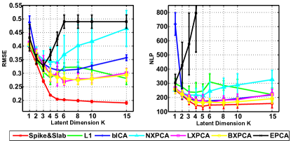
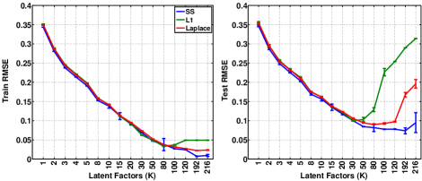
Figure 2 shows the NLP and RMSE on this benchmark data set. The methods developed are compared to EPCA [6], BXPCA [23] and to binary ICA [15]. A random predictor would have an bits. The models tested here have performance significantly better than this. Both optimisation-based and Bayesian learning approaches do well, but the spike-and-slab model shows the best performance with smaller error bars.
6.2 Real Data
We summarise the real data sets we use in table 1 (which includes data in the regime).
| # | Data | N | D | Type |
|---|---|---|---|---|
| 1 | Natural scenes | 10,000 | 144 | Real |
| 2 | Animal attributes | 33 | 102 | Binary |
| 3 | Newsgroups | 100 | 200 | Counts |
| 4 | Hapmap | 100 | 200 | Binary |
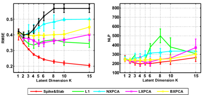
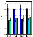
Natural images are the topic of much research based on regularisation. For the Olshausen and Field [26] image data set, we use image patches extracted from a set of larger images. We use the Gaussian instantiation of the sparse generalised model (equation 2) and evaluate the performance of: optimisation; a Laplace-prior factor model; and the Bayesian spike-and-slab model. Our results are shown for both underdetermined and overcomplete bases (K = 192 as in Olshausen and Field [26]) in figure 2. All methods perform similarly in the low-rank approximation cases, but as the model becomes overcomplete, Bayesian methods perform better with the spike-and-slab method much better than other methods, particularly in reconstructing held-out/missing data. The animal attributes data set of Kemp and Tenenbaum [16] consists of animal species with ecological and biological properties as features. We use the binary unsupervised model and show results for various latent dimensions for NLP and RMSE in figure 3. For this data, the NLP of a random classifier is 336 bits and the models have NLP values much lower than this.
| K | Spike-Slab | |
|---|---|---|
| 5 | 475 36 | 1446 24 |
| 6 | 48357 | 1418 29 |
| 8 | 592207 | 140018 |
| 10 | 934440 | 136732 |
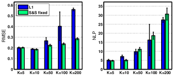
We also use a subset of the popular 20 newsgroups data set, consisting of documents and counts of the words used in each document, with data sparsity of 93%. Figure 4(b) shows the performance of the Poisson unsupervised model using and spike-and-slab. Apart from the application of the model to count data, the results show that the spike-and-slab model is able to deal effectively with the sparse data and provides effective reconstructions and good predictive performance on held out data. We are also able to show the improved behaviour of the spike-and-slab model using the Hapmap data set222Obtained from: https://mathgen.stats.ox.ac.uk/impute/. The comparative performance is shown in figure 4(c) showing the spike-and-slab has performance similar to in terms of RMSE at low , but much better performance for large .
7 Discussion and Conclusion
The common lore when using MCMC is that it is dramatically slower than optimisation methods. For optimisation methods, the cross-validation procedure needed to set regularisation parameters and , is computationally demanding due to the need to execute the optimisation for many combinations of parameters. This approach is also wasteful of data, since a separate validation data set is needed to make sensible choices of these values and to avoid model overfitting. While individual optimisations may be quick, the overall procedure can take an extended time, which depends on the granularity of the grid over which regularisation values are searched for. These parameters can be learnt in the Bayesian setting and have the advantage that we obtain information about the distribution of our latent variables, rather than point estimates and can have significantly better performance.
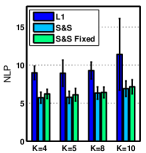
Figure 4 demonstrates this tradeoff between running time and performance of the optimisation and the Bayesian approaches. was allowed to run to convergence and the spike-and-slab for 200 iterations. In this instance, the Bayesian method is seemingly slower, but produced significantly better reconstructions in both the human judgements and newsgroups data. We considered the setting where we have a fixed time budget and fixed the running time for the spike-and-slab to that used by the model (including time to search for hyperparameters). The result is shown (as S&S fixed) in figure 4, which shows that even with a fixed time budget, MCMC performs better in this setting. The table of figure 4(d) shows that the number of non-zeroes in the reconstructions for various for the newsgroups data, with the true number of non-zeroes being 1436. is poor in learning the structure of this sparse data set, whereas the spike-and-slab is robust to the data sparsity.
All our results showed the spike-and-slab approach to have better performance than other methods compared in the same model class. The models based on the norm or Bayesian models with continuous sparsity favouring priors enforce global shrinkage on parameters of the model. It is this property that induces the sparsity property, but which also results in the shrinkage of parameters of relevance to the data. This can be problematic in certain cases, such as the newsgroups data set which resulted in overly sparse data reconstructions. The spike-and-slab has the ability to give both global and local shrinkage, thus allowing sparsity in the model parameters while not restricting parameters that contribute to explaining the data.
Current approaches for sparse learning will have difficulty scaling to large data sets in this regime. We might think of EP as a potential solution, such as used by Hernández Lobato et al. [12], but this is restricted to regression problems. For the standard Gaussian model, Rattray et al. [28] discuss this issue and propose a hybrid VB-EP approach as one way of achieving fast inference, but such an approach is not ideal, leaving scope for future work.
We have demonstrated that improved performance can be obtained by considering sparse Bayesian approaches. In particular, Bayesian learning with spike-and-slab priors consistently showed the best performance on held out data and produced accurate reconstructions, even in the ‘large ’ paradigm or with restricted running times. By considering the broad family of unsupervised latent variable models, we developed a sparse generalised model and provided new sampling methods for sparse Bayesian learning using the spike-and-slab distribution. Importantly, we have provided the first comparison of sparse unsupervised learning using three approaches: optimisation using the norm, Bayesian learning using continuous sparsity favouring priors, and Bayesian learning using the spike-and-slab prior. We have also demonstrated our methods in diverse applications including text modelling, image coding and psychology showing the flexibility of the sparse models developed. These results show that Bayesian sparsity and spike-and-slab methods warrant a more prominent role and wider use in sparse modelling applications.
Acknowledgements
Support for: SM by the Canadian Institute for Advanced Research (CIFAR); KAH by an NSF Postdoctoral Fellowship; ZG by EPSRC EP/I036575/1.
References
- Airoldi et al. [2008] E. M. Airoldi, D. M. Blei, S. E. Fienberg, and E. P. Xing. Mixed membership stochastic blockmodels. Journal of Machine Learning Research, 9:1981–2014, 2008.
- Archambeau and Bach [2009] C. Archambeau and F. Bach. Sparse probabilistic projections. In NIPS. 2009.
- Candes [2006] E. J. Candes. Compressive sampling. In Proc. Int. Con. Math, 2006.
- Carvalho et al. [2010] C. Carvalho, N. Polson, and J. Scott. The horseshoe estimator for sparse signals. Biometrika, 97(2), 2010.
- Carvalho et al. [2008] C. M. Carvalho, J. Chang, J. E. Lucas, J. R. Nevins, Q. Wang, and M. West. High-dimensional sparse factor modeling: Applications in gene expression genomics. J. Am. Stat. Ass., 103(484):1438–1456, 2008.
- Collins et al. [2002] M. Collins, S. Dasgupta, and R. Schapire. A generalization of principal components to the exponential family. In NIPS 14, pages 617 – 624, 2002.
- Courville et al. [2010] A. Courville, J. Bergstra, and Y. Bengio. A spike and slab restricted Boltzmann machine. In AISTATS 14. 2010.
- d’Aspremont et al. [2005] A. d’Aspremont, L. El Ghaoui, M. I. Jordan, and G. R.G. Lanckriet. A direct formulation for sparse PCA using semidefinite programming. In NIPS 17, 2005.
- Dueck and Frey [2004] D. Dueck and B. Frey. Probabilistic sparse matrix factorization. Technical report, Univ. Toronto, 2004.
- Griffiths and Ghahramani [2006] T. Griffiths and Z. Ghahramani. Infinite latent feature models and the Indian Buffet Process. In NIPS 19, 2006.
- Guihenneuc-Jouyaux and Rousseau [2005] C. Guihenneuc-Jouyaux and J. Rousseau. Laplace expansions in Markov chain Monte Carlo algorithms. J. Comp. Grap. Stats, 14(1):pp. 75–94, 2005.
- Hernández Lobato et al. [2010] D. Hernández Lobato, J. Hernández-Lobato, T. Helleputte, and P. Dupont. Expectation propagation for Bayesian multi-task feature selection. Machine Learning and Knowledge Discovery in Databases, pages 522–537, 2010.
- Ishwaran and Rao [2005] H. Ishwaran and J. S. Rao. Spike and Slab variable selection: Frequentist and Bayesian strategies. Annals of Statistics, 33(2):730–773, 2005.
- Johnstone and Silverman [2004] I. M. Johnstone and B. W. Silverman. Needles and straw in haystacks: Empirical Bayes estimates of possibly sparse sequences. Ann. Stat., 32(4):1594–1694, 2004.
- Kaban and Bingham [2006] A. Kaban and E. Bingham. ICA-based binary feature construction. In ICA 6, 2006.
- Kemp and Tenenbaum [2008] C. Kemp and J. B. Tenenbaum. The discovery of structural form. PNAS, 105(31):10687–10692, 2008.
- Lee et al. [2009] H. Lee, R. Raina, A. Teichman, and A. Y. Ng. Exponential family sparse coding with applications to self-taught learning. In IJCAI’09, pages 1113–1119, 2009.
- Lee et al. [2006] S. Lee, H. Lee, P. Abbeel, and A.Y. Ng. Efficient L1 regularized logistic regression. In AAAI-06. 2006.
- Levin et al. [2009] A. Levin, Y. Weiss, F. Durand, and W. T. Freeman. Understanding and evaluating blind deconvolution algorithms. In CVPR, 2009.
- Lücke and Sheikh [2012] J. Lücke and A Sheikh. Closed-form EM for sparse coding and its application to source separation. In LVA/ICA, 2012.
- MacKay [2003] D. J. C. MacKay. Information Theory, Inference & Learning Algorithms. Cambridge Press, 2003.
- Mitchell and Beauchamp [1988] T. J. Mitchell and J. J. Beauchamp. Variable selection in linear regression (with discussion). Journal of the American Statistical Association, 83:1023–1036, 1988.
- Mohamed et al. [2008] S. Mohamed, K. Heller, and Z. Ghahramani. Bayesian exponential family PCA. In NIPS 21, 2008.
- Neal [2003] R. M. Neal. Slice sampling. Ann. Stat., 31(3), 2003.
- O’Hara and Sillanpäa [2009] R. B. O’Hara and M. J. Sillanpäa. A review of Bayesian variable selections methods: What, how and which. Bayesian Analysis, 4(1):85 – 118, 2009.
- Olshausen and Field [1996] B. A. Olshausen and D. J. Field. Emergence of simple-cell receptive field properties by learning a sparse code for natural images. Nature, 381(6583):607–609, June 1996.
- Polson and Scott [2010] N. G. Polson and J. G. Scott. Shrink globally, act locally: Sparse Bayesian regularization and prediction. In Bayesian Statistics, volume 9. 2010.
- Rattray et al. [2009] M. Rattray, O. Stegle, K. Sharp, and J. Winn. Inference algorithms and learning theory for Bayesian sparse factor analysis. 2009.
- Schmidt et al. [2007] M. Schmidt, G. Fung, and R. Rosales. Fast optimization methods for L1 regularization: A comparative study and two new approaches. In ECML-2006. Springer, 2007.
- Seeger. et al. [2007] M. Seeger., F. Steinke, and K. Tsuda. Bayesian inference and optimal design in the sparse linear model. In AISTATS 11, pages 444–451, 2007.
- Tibshirani [1996] R. Tibshirani. Regression shrinkage and selection via the LASSO. JRSS B, 58(1):267–288, 1996.
- van de Geer and Bühlmann [2009] S. A. van de Geer and P. Bühlmann. On the conditions used to prove oracle results for the Lasso. Electronic Journal of Statistics, 3:1360–1392, 2009.
- Wipf and Nagarajan [2008] D. Wipf and S. Nagarajan. A new view of automatic relevance determination. In NIPS 20, 2008.
- Yen [2011] T.J. Yen. A majorization–minimization approach to variable selection using spike and slab priors. The Annals of Statistics, 39(3):1748–1775, 2011.
- Zou et al. [2004] H. Zou, T. Hastie, and R. Tibshirani. Sparse PCA. Technical report, Stanford U., 2004.