On the accuracy of solving confluent Prony systems

Abstract

In this paper we consider several nonlinear systems of algebraic equations which can be called “Prony-type”. These systems arise in various reconstruction problems in several branches of theoretical and applied mathematics, such as frequency estimation and nonlinear Fourier inversion. Consequently, the question of stability of solution with respect to errors in the right-hand side becomes critical for the success of any particular application. We investigate the question of “maximal possible accuracy” of solving Prony-type systems, putting stress on the “local” behavior which approximates situations with low absolute measurement error. The accuracy estimates are formulated in very simple geometric terms, shedding some light on the structure of the problem. Numerical tests suggest that “global” solution techniques such as Prony’s algorithm and ESPRIT method are suboptimal when compared to this theoretical “best local” behavior.

1 Introduction

1.A Problem definition

Consider the following system of algebraic equations:

$$\sum_{i=1}^{\mathcal{K}}a_{i}\xi_{i}^{k} =m_{k}$$ (1)

where $a_{i},\xi_{i}\in\mathbb{C}$ are unknown parameters and the measurements $\left\{m_{k}\right\}_{k=0,1,\dotsc,}$ are given. This “exponential fitting” system, or “Prony system”, appears in several branches of theoretical and applied mathematics, such as frequency estimation, Padé approximation, array processing, statistics, interpolation, quadrature, radar signal detection, error correction codes, and many more. The literature on this subject is huge (for instance, the bibliography on Prony’s method from [3] is some 50+ pages long). Our interest in this system (and other, more general systems of this kind, to be specified below) is motivated by its central role in Algebraic Sampling – a recent approach to reconstruction of non-linear parametric models from measurements. There, it arises as the problem of reconstructing a signal modeled by a linear combination of Dirac $\delta$-distributions:

$$f(x) =\sum_{i=1}^{\mathcal{K}}a_{i}\delta(x-\xi_{i}),\quad a_{i},\xi_{i}\in\mathbb{R}$$ (2)

from the measurements given by the power moments

$$m_{k}(f)\stackrel{{\scriptstyle\text{def}}}{{=}}\int_{0}^{1}x^{k}f(x)\operatorname{d}x.$$ (3)

While the above problem may be considered mainly of theoretical interest, it is actually one of the most basic ones in Algebraic Sampling. On one hand, if $s(x)$ is a piecewise-constant signal with jump discontinuities at the locations $\xi_{1},\dotsc,\xi_{\mathcal{K}}$, then $s^{\prime}(x)=f(x)$ as in (2). Thus, the “signal” $f(x)$ essentially captures the non-smooth nature of $s(x)$. On the other hand, the moments (3) are convenient to consider because of the respective simplicity of the arising algebraic equations, while other types of measurements (e.g. Fourier coefficients) may be recast into moments after change of variables.

An important generalization of the Prony system, which is of great interest to us, arises when the simple model (2) is extended to include higher-order derivatives (see [8, 46] for examples of such constructions):

$$f(x) =\sum_{i=1}^{\mathcal{K}}\sum_{j=0}^{l_{i}-1}a_{ij}\delta^{(j)}(x-\xi_{i}),\quad a_{i,j},\xi_{j}\in\mathbb{R}$$ (4)

where $\delta^{(j)}$ is the $j$-th derivative of the Dirac delta (in the sense of distributions).

From now on, we denote the number of unknown coefficients $a_{i,j}$ by $C\stackrel{{\scriptstyle\text{def}}}{{=}}\sum_{i=1}^{\mathcal{K}}l_{i}$, and the overall number of unknown parameters by $R\stackrel{{\scriptstyle\text{def}}}{{=}}C+\mathcal{K}$. Taking moments of $f\left(x\right)$ in (4), we arrive at the following “confluent Prony” system:

$$\sum_{i=1}^{\mathcal{K}}\sum_{j=0}^{l_{i}-1}a_{i,j}(k)_{j}\xi_{i}^{k-j}=m_{k}\qquad a_{ij},\xi_{i},m_{k}\in\mathbb{C}$$ (5)

where the Pochhammer symbol $(i)_{j}$ denotes the falling factorial

$$(i)_{j}=i(i-1)\cdot\dotsc\cdot(i-j+1),\qquad i\in\mathbb{R},\;j\in\mathbb{N}$$

and the expression $(k)_{j}\xi_{i}^{k-j}$ is defined to be zero for $k>j$.

The Prony-type systems appear in various recent reconstruction methods of signals with discontinuities - see [7, 8, 9, 10, 11, 14, 18, 20, 21, 23, 24, 28, 32, 30]. In particular, Finite Rate of Innovation (FRI) techniques [19, 31, 46] have spawned a rather extensive literature (see e.g. a recent addition [44]). Usually, the $\xi_{i}$ represent “location” parameters of the problem, such as discontinuity locations or complex frequencies $\xi_{j}=\operatorname{e}^{\imath\omega_{j}}$. These variables enter the equations in a nonlinear way, and we call them “nodes”. The coefficients $a_{ij}$, on the other hand, enter the equations linearly, and we call them “magnitudes”.

While Algebraic Sampling provides exact reconstruction for noise-free data in many cases mentioned above, a critical issue remains - namely, stability, or accuracy of solution. Stable solution of Prony-type systems is generally considered to be a difficult problem, and in recent years many algorithms have been devised for this task (e.g. [6, 25, 26, 33, 34, 36, 38, 42, 45]). Perhaps the simplest version of the stability problem can be formulated as follows (cf. Definition 10, Definition 11 and Subsection 1.D).

Assume that the measurements $\left\{m_{k}\right\}_{k=0,\dots,S-1}$ are known with some error: $m_{k}+\varepsilon_{k}$. Given an estimate $\varepsilon=\max_{k}|\varepsilon_{k}|$, how large can the error in the reconstructed model parameters (i.e. $\left|\Delta\xi_{j}\right|\stackrel{{\scriptstyle\text{def}}}{{=}}|\widetilde{\xi_{j}}-\xi_{j}|$ and $\left|\Delta a_{i,j}\right|\stackrel{{\scriptstyle\text{def}}}{{=}}|\widetilde{a_{i,j}}-a_{i,j}|$) be in the worst case in terms of $\epsilon$, number of measurements $S$ and the true parameters $\left\{\xi_{j}\right\},\left\{a_{i,j}\right\}$?

In more detail, our ultimate goal may be described as follows:

1. determine the qualitative dependence of the accuracy on the values of the parameters;

2. quantify this dependence as precisely as possible;

3. determine how (and if at all) increasing the number of measurements (i.e. oversampling) improves accuracy.

1.B Related work

Matching the ubiquity of Prony-type systems is the impressive body of literature devoted to both designing methods of solution and analyzing the accuracy/robustness of these methods, see references above. Although there appears to be no simple answer to the above question of “maximal possible accuracy”, several important results in this direction are available in the literature, which we now briefly discuss.

Methods of solution can be roughly divided into three categories (see e.g. [41],[43, Section 4]): direct nonlinear minimization (nonlinear least squares), recurrence-based methods (such as original Prony’s method - see Section 2) and subspace methods (such as Pisarenko’s method, MUSIC, ESPRIT, matrix pencils - see e.g. [38]).

In the framework of statistical signal estimation [27], the subspace methods are known to be more efficient and robust to noise, mainly due to the fact that the noise is assumed to have certain statistical properties. The confluent Prony system (5) is also known as “polynomial amplitude complex exponential” (PACE) model. A standard measure of estimator performance is Cramer-Rao (and related) lower bounds (CRB). These have been recently established for the PACE model in [5] (see also related results for FRI models [15]). Furthermore, it has been demonstrated that the performance of the generalized ESPRIT algorithm ([4, 6] and Subsection 5.B) is close to the optimal CRB, therefore we consider it to represent the state of the art in the subspace methods.

We do not assume any particular statistical model or other structure for either the error terms $\varepsilon_{k}$ or the estimation algorithm (such as white noise or unbiasedness). Therefore, the CRB and related lower bounds cannot provide the full answer to the stability problem as is. Still, it turns out that the stability bounds developed in this paper resemble the CRB as established in [5], see Subsection 5.A below for details.

Recent papers of Tasche et al. [34, 36] contain some uniform error bounds for solving Prony systems. In particular, the authors develop the so-called Approximate Prony method, analyze its worst-case error and numerically compare it with the ESPRIT method (showing similar performance). Although they consider the non-confluent version of the Prony system (1) and analyze only the error in recovering the magnitudes $a_{j}$, we believe these results to be an important step towards answering the stability problem as posed above. See Subsection 5.C below for details.

Very recently, Candes et al. [18] investigated stable solution of Prony systems by total variation minimization under assumptions of minimal node separation, in the context of super-resolution.

Considering all the above, we believe that a full answer to our somewhat rigid $l^{\infty}$ formulation of the stability problem may contribute to the understanding of limitations of using Prony systems and methods both in signal processing applications and in function approximation, in particular compressed sensing, nonlinear Fourier inversion, Finite Rate of Innovation techniques and related problems.

1.C Notation

In the sequel we use the infinity norm distance

$$\forall{\boldsymbol{x}},{\boldsymbol{y}}\in\mathbb{C}^{n}:\qquad\operatorname{dist}\left({\boldsymbol{x}},{\boldsymbol{y}}\right)\stackrel{{\scriptstyle\text{def}}}{{=}}\max_{1\leq i\leq n}\left|x_{i}-y_{i}\right|,$$

and denote by $B\left({\boldsymbol{a}},\varepsilon\right)$ the $\varepsilon$-ball around a point ${\boldsymbol{a}}\in\mathbb{C}^{n}$ in this norm.

1.D Summary of results

In Section 3 we define “best possible point-wise accuracy” as follows. We consider the “Prony map” $\mathcal{P}_{S}:\mathbb{C}^{R}\to\mathbb{C}^{S}$ which associates to any parameter vector ${\boldsymbol{x}}=\bigl{\{}\{a_{ij}\},\{\xi_{i}\}\bigr{\}}\in\mathbb{C}^{R}$ its corresponding measurement vector ${\boldsymbol{y}}=\left(m_{0},\dots,m_{S-1}\right)\in\mathbb{C}^{S}$ (where the $m_{k}$ are given by (5)).

Now if instead of ${\boldsymbol{y}}$ we are given a noisy $\tilde{{\boldsymbol{y}}}\in B\left({\boldsymbol{y}},\varepsilon\right)$, then this $\tilde{{\boldsymbol{y}}}$ can correspond to any parameter vector $\tilde{{\boldsymbol{x}}}\in\mathbb{C}^{R}$ for which $\mathcal{P}_{S}\left(\tilde{{\boldsymbol{x}}}\right)\in B\left(\tilde{{\boldsymbol{y}}},\varepsilon\right)$. Therefore we define the best possible accuracy at a point ${\boldsymbol{x}}$ to be equal to the maximal (over all $\tilde{{\boldsymbol{y}}})$ spread of the preimage of this $B\left(\tilde{{\boldsymbol{y}}},\varepsilon\right)$, that is (see Definition 10)

$$\sup_{\tilde{{\boldsymbol{y}}}\in B\left({\boldsymbol{y}},\varepsilon\right)}\frac{1}{2}\operatorname{diam}\mathcal{P}_{S}^{-1}\left(B\left(\tilde{{\boldsymbol{y}}},\varepsilon\right)\right).$$

We then simplify the setting by assuming that the number of measurements $S$ equals the number of unknowns $R$, and looking at the (local) linear approximation to the Prony map $\mathcal{P}_{S}$. Then the solution error at some (non-critical) point in the parameter space can be estimated by the local Lipschitz constant of the (regular) inverse map $\mathcal{P}_{S}^{-1}$. We derive such simple estimates in Section 4, and compare them to the “global” accuracy of the original Prony method (derived for completeness in Section 2).

Our main result (Theorem 15) can be summarized as follows (all statements are valid for small $\varepsilon$):

1. The stability of recovering a node $\xi_{i}$ depends on the separation of the nodes and is inversely proportional to the magnitude of the highest coefficient corresponding to this node ($\left|a_{i.l_{i}-1}\right|$), and does not depend on any other magnitude.

2. For $1\leq j\leq l_{i}-1$, the stability of recovering a magnitude $a_{i,j}$ depends on the separation of the nodes, is proportional to $1+\frac{\left|a_{i,j-1}\right|}{\left|a_{i,l_{i}-1}\right|}$, and does not depend on any other magnitude. Note that in fact every magnitude influences only the next highest magnitude corresponding to the same node.

3. The stability of recovering the lowest magnitudes $a_{i,0}$ is the same for all nodes and it depends only on the separation of the nodes.

The separation of the nodes is specified in terms of norms of inverse confluent Vandermonde matrices on the nodes, which is roughly of the same order as some finite power of $\prod_{1\leq i<j\leq\mathcal{K}}\left|\xi_{j}-\xi_{i}\right|^{-1}$.

Our numerical experiments (Section 6) confirm the above theoretical estimates. We also test the performance of two well-known solution methods - namely the recurrence-based Prony method (Section 2) and the generalized ESPRIT (Subsection 5.B) - in the same setting as above (i.e. high SNR). The results suggest that:

1. The recurrence-based global Prony method does not achieve the above theoretical limits, and so it is not optimal even in the case of small data perturbations.

2. The subspace methods (in particular the ESPRIT algorithm) behave better than the Prony method but still they are not optimal for small perturbations and small sample size.

The “Prony map” approach can in principle be generalized to obtain both global accuracy bounds as well as study effects of oversampling - by considering the case $S>R$ and taking into account second-order terms in the Taylor expansion of $\mathcal{P}_{S}$. We discuss these directions in Section 7.

1.E Acknowledgments

We are grateful to the two anonymous referees, whose comments, suggestions and references were very helpful.

2 The Prony method

In this section we describe the most basic solution method for the system (5), which is in fact a slight generalization of the (historically earliest) method due to Prony [37]. By factorizing the so-called “data matrix”, one immediately obtains necessary and sufficient conditions for a unique solution, as well as an estimate of the numerical stability of the method.

Most of the results of Section 2 are not new and are scattered throughout the literature. Nevertheless, we believe that our presentation can be useful for further study of the various singular situations, such as collision of two nodes.

2.A The description of the method

The non-trivial part is the recovery of the nodes $\xi_{j}$. Note that the case of a-priori known nodes has been extensively treated in the literature (see e.g. [1, 35] for the most recent results). Using the framework of finite difference calculus, one can easily prove the following result (see [8, Theorem 2.8]).

Proposition 1.

Let the sequence $\{m_{k}\}$ be given by (5). Then this sequence satisfies the recurrence relation (of length at most $C+1$)

$$\biggl{(}\prod_{i=1}^{\mathcal{K}}(\operatorname{E}-\xi_{i}\operatorname{I})^{l_{i}}\biggr{)}\{m_{k}\} =0$$

where $\operatorname{E}$ is the forward shift operator in $k$ and $\operatorname{I}$ is the identity operator.

Corollary 2.

For all $k\in\mathbb{N}$ we have the recurrence relation $\sum_{j=0}^{C}q_{j}m_{k+j}=0$ where $q_{0},q_{1},\dots,q_{C}$ are the coefficients of the polynomial $q(x)\stackrel{{\scriptstyle\text{def}}}{{=}}\prod_{i=1}^{\mathcal{K}}(x-\xi_{i})^{l_{i}}$.

This suggests the following reconstruction procedure.

Let there be given $\{m_{k}\}_{k=0}^{2C-1}$ (where $C=\sum_{i=1}^{\mathcal{K}}l_{i}$).

1. Solve the linear system (here we set $q_{C}=1$ for normalization)

   $$\underbrace{\begin{pmatrix}m_{0}&m_{1}&\cdots&m_{C-1}\\ m_{1}&m_{2}&\cdots&m_{C}\\ \vdots&\vdots&\vdots&\vdots\\ m_{C-1}&m_{C}&\cdots&m_{2C-2}\end{pmatrix}}_{\stackrel{{\scriptstyle\text{def}}}{{=}}M_{C}}\begin{pmatrix}q_{0}\\ q_{1}\\ \vdots\\ q_{C-1}\end{pmatrix}=-\begin{pmatrix}m_{C}\\ m_{C+1}\\ \vdots\\ m_{2C-1}\end{pmatrix}$$ (6)

   for the unknown coefficients $q_{0},\dotsc,q_{C-1}$.

2. Find all the roots of $q(x)=x^{C}+\sum_{j=0}^{C-1}q_{i}x^{i}$. These roots, with appropriate multiplicities, are the unknowns $\xi_{1},\dotsc,\xi_{\mathcal{K}}$ (use e.g. arithmetic means to estimate multiple roots which are scattered by the noise into clusters).

3. Substitute the recovered $\xi_{i}$’s back into the original equations (5). Solve the resulting overdetermined linear system ($C$ unknowns and $2C$ equations) with respect to the magnitudes $\left\{a_{i,j}\right\}$ by least squares method.

Algorithm 1 The Prony method

Several comments are in order.

1. The number of measurements used in step 1 equals $2C$ which can be greater than the number of unknowns $R=C+\mathcal{K}$ (equality for order zero Prony system). If more measurements are available, the linear system (6) can be modified in a straightforward way to be overdetermined, and subsequently solved by, say, the least squares method.

2. The linear system for the magnitudes has a special “Vandermonde”-like structure (see below), and so certain efficient algorithms can be used to solve it (e.g. [16, 29]).

The remainder of this section is organized as follows. The Hankel matrix $M_{C}$ is shown to factor into the product of a generalized “Vandermonde-type” matrix which depends only on the nodes $\xi_{j}$, with a upper triangular matrix depending only on the amplitudes $a_{i,j}$. We also write down explicitly the linear system for the $a_{i,j}$ (see step 3 in Algorithm 1 above). These calculations lead to simple non-degeneracy conditions and stability estimates for the Prony method.

2.B Factorization of the data matrix

Let us start by recalling a well-known type of matrices.

Definition 3.

For every $j=1,\dotsc,\mathcal{K}$ and $k\in\mathbb{N}$ let the symbol ${\boldsymbol{u}_{j,k}}$ denote the following $1\times l_{j}$ row vector

$${\boldsymbol{u}_{j,k}}\stackrel{{\scriptstyle\text{def}}}{{=}}\left[\begin{array}[]{cccc}\xi_{j}^{k},&k\xi_{j}^{k-1},&\dots&,(k)_{l_{j}-1}\xi_{j}^{k-l_{j}+1}\end{array}\right].$$ (7)

Definition 4.

Let $U=U(\xi_{1},l_{1},\dotsc,\xi_{\mathcal{K}},l_{\mathcal{K}})$ denote the matrix

$$U=\left[\begin{array}[]{cccc}{\boldsymbol{u}_{1,0}}&{\boldsymbol{u}_{2,0}}&\dotsc&{\boldsymbol{u}_{\mathcal{K},0}}\\ {\boldsymbol{u}_{1,1}}&{\boldsymbol{u}_{2,1}}&\dotsc&{\boldsymbol{u}_{\mathcal{K},1}}\\ &&\dotsc\\ {\boldsymbol{u}_{1,C-1}}&{\boldsymbol{u}_{2,C-1}}&\dotsc&{\boldsymbol{u}_{\mathcal{K},C-1}}\end{array}\right].$$ (8)

This matrix is called the “confluent Vandermonde” ([16, 22]) matrix. It has been long known in numerical analysis due to its central role in Hermite polynomial interpolation. Its determinant is ([40, p.30])

$$\det U=\prod_{1\leq i<j\leq\mathcal{K}}(\xi_{j}-\xi_{i})^{l_{j}l_{i}}\prod_{\mu=1}^{\mathcal{K}}\prod_{\nu=1}^{l_{\mu}-1}\nu!.$$ (9)

It is straightforward to see that the matrix $U$ defines the linear system for the jump magnitudes $a_{i,j}$.

Proposition 5.

Let ${\boldsymbol{a}}$ be the column vector containing all the magnitudes $\left\{a_{i,j}\right\}$, i.e.

$${\boldsymbol{a}}\stackrel{{\scriptstyle\text{def}}}{{=}}[a_{1,0},\dots,a_{1,l_{1}-1},a_{2,0},\dots,a_{2,l_{2}-1},\dots,a_{\mathcal{K},0},a_{\mathcal{K},l_{\mathcal{K}}-1}]^{T}$$

and ${\boldsymbol{m}}\stackrel{{\scriptstyle\text{def}}}{{=}}[m_{0},\dots,m_{C-1}]^{T}$. Then we have

$$U(\xi_{1},l_{1},\dotsc,\xi_{\mathcal{K}},l_{\mathcal{K}}){\boldsymbol{a}}={\boldsymbol{m}.}$$ (10)

It is known that every Hankel matrix $H$ admits a factorization $H=UDU^{T}$, where $U$ is given by (8) and $D$ is a block diagonal matrix – see [17]. Using different notations, such a factorization is proved in [4, Proposition III.7] for the Hankel matrix $M_{C}$.

Lemma 6.

For the system (5), the matrix $M_{C}$ admits the following factorization:

$$M_{C}=UBU^{T}$$ (11)

where $U=U(\xi_{1},l_{1},\dotsc,\xi_{\mathcal{K}},l_{\mathcal{K}})$ is the confluent Vandermonde matrix (8) and $B$ is the $C\times C$ block diagonal matrix $B=\operatorname{diag}\{B_{1},\dotsc,B_{\mathcal{K}}\}$ with each block of size $l_{i}\times l_{i}$ given by

$$B_{i}\stackrel{{\scriptstyle\text{def}}}{{=}}\begin{bmatrix}a_{i0}&a_{i1}&\cdots&\cdots&a_{i,l_{i}-1}\\ a_{i1}&&&{l_{i}-1\choose l_{i}-2}a_{i,l_{i}-1}&0\\ \cdots&&&\cdots&0\\ &{l_{i}-1\choose 2}a_{i,l_{i}-1}&0&\cdots&0\\ a_{i,l_{i}-1}&0&\cdots&\cdots&0\end{bmatrix}.$$ (12)

In other words, $B_{i}$ is a “flipped” upper triangular matrix whose $j$-th anti-diagonal equals to

$$a_{ij}\cdot\begin{bmatrix}1&{j\choose 2}&\cdots&\ {j\choose j-1}&1\end{bmatrix}$$

for $j=0,\dotsc,l_{i}-1$.

The formula (11) is useful because it separates the jump locations $\{\xi_{i}\}$ from the magnitudes $\{a_{i,j}\}$, simplifying the analysis considerably.

Theorem 7.

The system (5) for $k=0,1,\dots,2C$ has a unique solution if and only if all the $\left\{\xi_{i}\right\}$’s are pairwise different and all the $\left\{a_{i,l_{i}-1}\right\}$’s (just the highest coefficients) are nonzero.

Proof.

Existence of a unique solution to the system (6) is equivalent to the non-degeneracy of $M_{C}=UBU^{T}$. Furthermore, the system for the jump magnitudes is given by (10). Therefore, existence of a unique solution to (5) is equivalent to the conditions $\det U\neq 0$ and $\det B\neq 0$. The proof is completed by (9) and (12). ∎

2.C Stability estimates

The stability of the Prony method can be estimated by the condition numbers of the matrices $B$ and $U$. In particular, we have the following well-known result (e.g. [47]) from numerical linear algebra.

Lemma 8.

Consider the linear system $A{\boldsymbol{x}}={\boldsymbol{b}}$ and let ${\boldsymbol{x}_{0}}$ be the exact solution. Let this system be perturbed:

$$\left(A+\Delta A\right){\boldsymbol{x}}={\boldsymbol{b}}+{\boldsymbol{\Delta}b}$$

and let ${\boldsymbol{x}_{0}}+{\boldsymbol{\Delta}x}$ denote the exact solution of this perturbed system. Denote $\delta x=\frac{\|{\boldsymbol{\Delta}x}\|}{\|{\boldsymbol{x}_{0}}\|},\delta A=\frac{\|\Delta A\|}{\|A\|},\delta b=\frac{\|{\boldsymbol{\Delta}b}\|}{\|{\boldsymbol{b}}\|}$ and the condition number $\kappa=\|A\|\|A^{-1}\|$ for some vector norm $\|\cdot\|$ and the induced matrix norm. Then

$$\delta x\leq\frac{\kappa}{1-\kappa\cdot\delta A}\left(\delta A+\delta b\right).$$ (13)

Now we can easily estimate the stability of the Prony method (compare with similar estimates in [4, eq. (19)]).

Corollary 9.

Let the measurements $\left\{m_{k}\right\}$ be given with an error bounded by $\varepsilon$. Denote $u=\kappa(U),b=\kappa(B)$. Assume that $\left|\xi_{i}\right|\leq\Xi$ for all $i=1,\dots,\mathcal{K}$. Then the Prony method recovers the parameters $\{\xi_{j},a_{i,j}\}$ with the following accuracy as $\varepsilon\to 0$:

$$|\Delta\xi_{j}| \sim\left(u^{2}b\varepsilon\right)^{\frac{1}{l_{j}}}+O\left(\varepsilon^{\frac{2}{l_{j}}}\right)$$

$$|\Delta a_{i,j}| \sim C\left(\Xi\right)u\left(u^{2}b\varepsilon\right)^{\frac{1}{\max_{j}l_{j}}}+\text{L.O.T.}$$

where $C\left(\Xi\right)$ is a constant depending on the number $\Xi$.

Proof.

Using the factorization of Lemma 6, we obtain that $\kappa\left(M_{C}\right)\leq u^{2}b$. Therefore, according to (13) the coefficient vector ${\boldsymbol{q}}=\left(q_{0},\dots,q_{C-1}\right)$ is recovered with the accuracy

$$\|\delta{\boldsymbol{q}}\| \sim\frac{\kappa\left(M_{C}\right)}{1-\kappa\left(M_{C}\right)\delta M_{C}}\cdot\bigl{(}\delta M_{C}+\delta{\boldsymbol{m}}\bigr{)}$$

$$\leq\frac{u^{2}b\varepsilon}{1-u^{2}b\varepsilon}\sim u^{2}b\varepsilon+O(\varepsilon^{2}).$$

The parameters $\xi_{1},\dots,\xi_{\mathcal{K}}$ are the roots of the polynomial with coefficient vector ${\boldsymbol{q}}$, with multiplicities $l_{1},\dots,l_{\mathcal{K}}$. Therefore, by the general theory of stability of polynomial roots (see e.g. [47]) it is known that $\Delta\xi_{j}\sim\left(\delta{\boldsymbol{q}}\right)^{\frac{1}{l_{j}}}$. The first part of the claim is thus proved.

Now consider the linear system (10) for recovering the jump magnitudes. Note that the matrix $U$ is known only approximately. Again, by (13) we have

$$\begin{split}\delta{\boldsymbol{a}}&\sim\frac{\kappa\left(U\right)}{1-\kappa\left(U\right)\delta U}\left(\delta U+\delta{\boldsymbol{m}}\right)\end{split}$$ (14)

Assuming that $\left|\xi_{j}\right|\leq\Xi$, it is easy to see that $\delta U\sim C\left(\Xi\right)\left(u^{2}b\varepsilon\right)^{\frac{1}{\max_{j}l_{j}}}$. Plugging this value into (14) we get the desired result. ∎

Inverses of confluent Vandermonde matrices and their condition numbers are extensively studied in numerical linear algebra (e.g. [12, 13, 22]). In general, $\kappa(U)$ will grow exponentially with $\mathcal{K}$ and will also depend on the “node separation” $\prod_{i\neq j}|\xi_{j}-\xi_{j}|^{-1}$. As for $\kappa(B)$, we are not aware of a general formula except for the simplest cases.

Finally, notice that the stability estimates of Corollary 9 suggest that when the Prony method is used, the parameters of the problem are “coupled” to each other, in the sense that the accuracy of recovering either a node $\xi_{i}$ or a magnitude $a_{i,j}$ will depend on the values of all the parameters at once. This undesired behavior is confirmed by our numerical experiments in Section 6.

3 Measurement set and the Prony map

Assume that the number of measurements is $S\geq R$ (where $R$ is the overall number of parameters in the confluent Prony system). Then we define $\mathcal{M}_{R,S}$ to be the set of all possible exact measurements, i.e.

$$\mathcal{M}_{R,S}\stackrel{{\scriptstyle\text{def}}}{{=}}\left\{\left(m_{0},m_{1},\dots,m_{S-1}\right):\quad m_{k}=\sum_{i=1}^{\mathcal{K}}\sum_{j=0}^{l_{i}-1}a_{i,j}(k)_{j}\xi_{i}^{k-j},\;a_{i,j}\in\mathbb{C},\;\xi_{j}\in\mathbb{C}\right\}\subset\mathbb{C}^{S}.$$

This $\mathcal{M}_{R,S}$ is the image of $\mathbb{C}^{R}$ under the “Prony map” $\mathcal{P}_{S}:\mathbb{C}^{R}\to\mathbb{C}^{S}$ defined as

$$\mathcal{P}_{S}\left(\{a_{ij}\},\{\xi_{i}\}\right)=\left(m_{0},m_{1},\dots,m_{S-1}\right):\quad m_{k}=\sum_{i=1}^{\mathcal{K}}\sum_{j=0}^{l_{i}-1}a_{i,j}(k)_{j}\xi_{i}^{k-j}.$$ (15)

Now let ${\boldsymbol{x}}=\bigl{\{}\{a_{ij}\},\{\xi_{i}\}\bigr{\}}\in\mathbb{C}^{R}$ be an unknown parameter vector and ${\boldsymbol{{\boldsymbol{y}}}=\mathcal{P}_{S}\left({\boldsymbol{x}}\right)\in\mathcal{M}_{R,S}}$ its corresponding exact measurement vector. The absolute error in each measurement is bounded from above by $\varepsilon$, therefore the actual measurement satisfies $\tilde{{\boldsymbol{y}}}\in B\left({\boldsymbol{y}},\varepsilon\right)$. Now consider the set

$$T_{\tilde{{\boldsymbol{y}}},\varepsilon}\stackrel{{\scriptstyle\text{def}}}{{=}}\mathcal{M}_{R,S}\cap B\left(\tilde{{\boldsymbol{y}}},\varepsilon\right)$$

of all possible noise-free measurements corresponding to the given noisy one $\tilde{{\boldsymbol{y}}}$. Any algorithm which receives this $\tilde{{\boldsymbol{y}}}$ as input will therefore produce worst-case error which is at least

$$\frac{1}{2}\operatorname{diam}\mathcal{P}_{S}^{-1}\left(T_{\tilde{{\boldsymbol{y}}},\varepsilon}\right)$$

where $\mathcal{P}_{S}^{-1}$ denotes the full preimage set.

This prompts us to make the following definition.

Definition 10.

Assign to each one of the parameters $\{a_{ij}\},\{\xi_{i}\}$ a unique index $1\leq p\leq R$. The best possible point-wise accuracy of solving the noisy confluent Prony system (5) with each noise component bounded above by $\varepsilon$ at the point ${\boldsymbol{x}}=\left(\{a_{ij}\},\{\xi_{i}\}\right)\in\mathbb{C}^{R}$ with respect to the parameter $p$ is defined to be

$$\mathcal{ACC}\left({\boldsymbol{x}},\varepsilon,p\right)\stackrel{{\scriptstyle\text{def}}}{{=}}\sup_{\tilde{{\boldsymbol{y}}}\in B\left(\mathcal{P}_{S}\left({\boldsymbol{x}}\right),\varepsilon\right)}\frac{1}{2}\operatorname{diam}_{p}\mathcal{P}_{S}^{-1}\left(\mathcal{M}_{R,S}\cap B\left(\tilde{{\boldsymbol{y}}},\varepsilon\right)\right)$$

where $\operatorname{diam}_{p}A$ is the diameter of the set $A$ along the dimension $p$.

Obviously, $\mathcal{ACC}\left({\boldsymbol{x}},\varepsilon\right)$ will depend on the point ${\boldsymbol{x}}\in\mathbb{C}^{R}$ in a nontrivial way because the chart $\mathcal{P}_{S}$ is nonlinear. Calculation of the function $\mathcal{ACC}$ may be considered as one possible answer to the stability problem posed in the Introduction.

4 Local accuracy

Having given the general definition of accuracy, in the remainder of this paper we restrict ourselves to the “local” setting in the following sense: we assume that $\varepsilon$ is small enough so that the set $\mathcal{M}_{R,S}$ can be approximated by the linear part of the Prony map, and furthermore we take $S=R$ so that the preimage will be given by the usual inverse function. For such an analysis to be valid, it should be done at non-critical points of $\mathcal{P}_{S}$ so that this map is locally invertible. By definition, the point ${\boldsymbol{x}}$ is a critical point of $\mathcal{P}_{S}$ if the Jacobian determinant of $\mathcal{P}_{S}$ vanishes at ${\boldsymbol{x}}$.

To summarize, let us give the following definition of the local accuracy which is nothing more than the first-order Taylor approximation to the inverse function $\mathcal{N}=\mathcal{P}_{S}^{-1}$ at a regular point of $\mathcal{P}_{S}$.

Definition 11.

Assume $S=R$. Let ${\boldsymbol{x}}=\left(\{a_{ij}\},\{\xi_{i}\}\right)\in\mathbb{C}^{R}$ be a regular point of $\mathcal{P}_{S}$ and assume $\varepsilon$ to be small enough so that that the inverse function $\mathcal{N}=\mathcal{P}_{S}^{-1}$ exists in $\varepsilon$-neighborhood of ${\boldsymbol{y}}=\mathcal{P}_{S}\left({\boldsymbol{x}}\right)$. Assign, as before, to each one of the parameters $\{a_{ij}\},\{\xi_{i}\}$ a unique index $1\leq p\leq R$. The best possible local point-wise accuracy of solving the noisy confluent Prony system (5) with each noise component bounded above by $\varepsilon$ at the point ${\boldsymbol{x}}$ with respect to the parameter $p$ is

$$\mathcal{ACC}_{LOC}\left({\boldsymbol{x}},\varepsilon,p\right)\stackrel{{\scriptstyle\text{def}}}{{=}}\sup_{\tilde{{\boldsymbol{y}}}\in B\left({\boldsymbol{y}},\varepsilon\right)}\left|\left[\mathcal{J}_{\mathcal{N}}({\boldsymbol{y}})\left(\tilde{{\boldsymbol{y}}}-{\boldsymbol{y}}\right)\right]_{p}\right|$$

where $\mathcal{J}_{\mathcal{N}}\left({\boldsymbol{y}}\right)$ is the Jacobian of $\mathcal{N}$ at the point ${\boldsymbol{y}}$ and $\left[{\boldsymbol{v}}\right]_{p}$ is the $p$-th component of the vector ${\boldsymbol{v}}$.

In Theorem 15 below we estimate the function $\mathcal{ACC}_{LOC}$. The key technical tool is the following factorization of the Jacobian of $\mathcal{P}_{S}$ which separates the nonlinear part depending on the nodes $\{\xi_{j}\}$ from the linear part which depends on the magnitudes $\{a_{i,j}\}$.

Lemma 12.

Let ${\boldsymbol{x}}=\left(\{a_{ij}\},\{\xi_{i}\}\right)\in\mathbb{C}^{R}$. Then

$$\mathcal{J}_{\mathcal{P}_{S}}({\boldsymbol{x}})=U(\xi_{1},l_{1}+1,\dotsc,\xi_{\mathcal{K}},l_{\mathcal{K}}+1)\cdot\operatorname{diag}\{D_{1},\dotsc,D_{\mathcal{K}}\}$$ (16)

where $U(\dotsc)$ is the confluent Vandermonde matrix (8), and $D_{i}$ is the $(l_{i}+1)\times(l_{i}+1)$ block

$$D_{i}\stackrel{{\scriptstyle\text{def}}}{{=}}\begin{bmatrix}1&0&0&\cdots&0\\ 0&1&0&\cdots&a_{i,0}\\ \vdots&\vdots&\vdots&\ \ddots&\vdots\\ 0&0&0&\cdots&a_{i,l_{i}-1}\end{bmatrix}.$$ (17)

Proof.

We have by (15)

$$\begin{split}\frac{\partial m_{k}}{\partial a_{ij}}&=(k)_{j}\xi_{i}^{k-j},\\ \frac{\partial m_{k}}{\partial\xi_{i}}&=\sum_{j=0}^{l_{i}-1}a_{ij}(k)_{j}(k-j)\xi_{i}^{k-(j+1)}=\sum_{j=1}^{l_{i}}a_{i,j-1}(k)_{j}\xi_{i}^{k-j}.\end{split}$$

The rest of the proof is just a straightforward calculation. ∎

Corollary 13.

${\boldsymbol{x}}=\left(\{a_{ij}\},\{\xi_{i}\}\right)\in\mathbb{C}^{R}$ is a critical point of $\mathcal{P}_{S}$ if and only if at least one of the following conditions is satisfied:

1. $\xi_{i}=\xi_{j}$ for any pair of indices $i\neq j$.

2. $a_{i,l_{i}-1}=0$ for any $1\leq i\leq\mathcal{K}$.

Corollary 14.

Let ${\boldsymbol{x}}\in\mathbb{C}^{R}$ be a regular point of $\mathcal{P}_{S}$. Then the Jacobian matrix of the inverse function $\mathcal{N}=\mathcal{P}_{S}^{-1}$ at ${\boldsymbol{y}}=\mathcal{P}_{S}({\boldsymbol{x}})$ is equal to

$$\mathcal{J}_{\mathcal{N}}({\boldsymbol{y}})=\left\{\mathcal{J}_{\mathcal{P}_{S}}\left({\boldsymbol{x}}\right)\right\}^{-1} =\frac{\partial(a_{10},\dotsc,a_{1,l_{1}-1},\xi_{1},\dotsc,a_{\mathcal{K},0},\dotsc,a_{\mathcal{K},l_{\mathcal{K}}-1},\xi_{\mathcal{K}})}{\partial(m_{0},\dotsc,m_{R-1})}$$

$$=\operatorname{diag}\{D_{1}^{-1},\dotsc,D_{\mathcal{K}}^{-1}\}\cdot U^{-1}(\xi_{1},l_{1}+1,\dotsc,\xi_{\mathcal{K}},l_{\mathcal{K}}+1)$$

where

$$D_{i}^{-1}=\begin{bmatrix}1&0&0&\cdots&0\\ 0&1&0&\cdots&(-1)^{l_{i}-1}\frac{a_{i,0}}{a_{i,l_{i}-1}}\\ \vdots&\vdots&\vdots&\ddots&\vdots\\ 0&0&0&\cdots&\frac{1}{a_{i,l_{i}-1}}\end{bmatrix}.$$ (18)

Now we are ready to formulate and prove our local stability result.

Theorem 15.

Assume $S=R$. Let ${\boldsymbol{x}}=\left(\{a_{ij}\},\{\xi_{i}\}\right)\in\mathbb{C}^{n}$ be a regular point of $\mathcal{P}_{S}$ and assume $\varepsilon$ to be small enough so that that the inverse function $\mathcal{N}=\mathcal{P}_{S}^{-1}$ exists in $\varepsilon$-neighborhood of ${\boldsymbol{y}}=\mathcal{P}_{S}\left({\boldsymbol{x}}\right)$.

Then there exists a positive constant $C_{1}$ depending only on $\xi_{1},\dotsc,\xi_{\mathcal{K}}$ and $l_{1},\dotsc,l_{\mathcal{K}}$ such that for all $i=1,\dots,\mathcal{K}$

$$\mathcal{ACC}_{LOC}\left({\boldsymbol{x}},\varepsilon,a_{ij}\right) =\begin{cases}C_{1}\varepsilon&j=0\\ C_{1}\varepsilon\biggl{(}1+\frac{|a_{i,j-1}|}{|a_{i,l_{i}-1}|}\biggr{)}&1\leq j\leq l_{i}-1\end{cases},$$

$$\mathcal{ACC}_{LOC}\left({\boldsymbol{x}},\varepsilon,\xi_{i}\right) =C_{1}\varepsilon\frac{1}{|a_{i,l_{i}-1}|}.$$

Proof.

Express the Jacobian matrix $\mathcal{J}_{\mathcal{N}}({\boldsymbol{y}})$ as

$$\mathcal{J}_{\mathcal{N}}({\boldsymbol{y}})=\begin{bmatrix}{\boldsymbol{s}}_{10}^{T}&\dotsc&{\boldsymbol{s}}_{1,l_{1}-1}^{T}&{\boldsymbol{t}}_{1}^{T}&\dotsc&{\boldsymbol{s}}_{n0}^{T}&\dotsc&{\boldsymbol{s}}_{\mathcal{K},l_{\mathcal{K}}-1}^{T}&{\boldsymbol{t}}_{\mathcal{K}}^{T}\end{bmatrix}^{T}$$

where

$${\boldsymbol{s}}_{ij} \stackrel{{\scriptstyle\text{def}}}{{=}}\begin{bmatrix}\frac{\partial a_{ij}}{\partial m_{0}}&\frac{\partial a_{ij}}{\partial m_{1}}&\dotsc&\frac{\partial a_{ij}}{\partial m_{S-1}}\end{bmatrix},$$

$${\boldsymbol{t}}_{i} \stackrel{{\scriptstyle\text{def}}}{{=}}\begin{bmatrix}\frac{\partial\xi_{i}}{\partial m_{0}}&\frac{\partial\xi_{i}}{\partial m_{1}}&\dotsc\frac{\partial\xi_{i}}{\partial m_{S-1}}\end{bmatrix}.$$

Let $\tilde{{\boldsymbol{y}}}=\left(m_{0}+\Delta m_{0},\dots,m_{S-1}+\Delta m_{S-1}\right)$ where each $\left|\Delta m_{k}\right|<\varepsilon$. Denote by $\|\cdot\|_{1}$ the $l_{1}$ vector norm, i.e. if ${\boldsymbol{v}}=(v_{i})$ is an $n$-vector then $\|{\boldsymbol{v}}\|_{1}\stackrel{{\scriptstyle\text{def}}}{{=}}\sum_{i=1}^{n}|v_{i}|$. Then

$$\left[\mathcal{J}_{\mathcal{N}}\left({\boldsymbol{y}}\right)\left(\tilde{{\boldsymbol{y}}}-{\boldsymbol{y}}\right)\right]_{a_{ij}} =\biggl{|}\sum_{k=0}^{P-1}\frac{\partial a_{ij}}{\partial m_{k}}\Delta m_{k}\biggr{|}\leq\varepsilon\|{\boldsymbol{s}}_{ij}\|_{1},$$

$$\left[\mathcal{J}_{\mathcal{N}}\left({\boldsymbol{y}}\right)\left(\tilde{{\boldsymbol{y}}}-{\boldsymbol{y}}\right)\right]_{\xi_{i}} =\biggl{|}\sum_{k=0}^{P-1}\frac{\partial\xi_{i}}{\partial m_{k}}\Delta m_{k}\biggr{|}\leq\varepsilon\|{\boldsymbol{t}}_{i}\|_{1}.$$

By Corollary 14, the matrix $\mathcal{J}_{\mathcal{N}}$ is the product of the block diagonal matrix $D^{*}\stackrel{{\scriptstyle\text{def}}}{{=}}\operatorname{diag}\{D_{1}^{-1},\dotsc,D_{\mathcal{K}}^{-1}\}$ with the matrix $U^{*}\stackrel{{\scriptstyle\text{def}}}{{=}}(U(\xi_{1},l_{1}+1,\dotsc,\xi_{\mathcal{K}},l_{\mathcal{K}}+1))^{-1}$. Therefore, ${\boldsymbol{s}}_{ij}$ and ${\boldsymbol{t}}_{i}$ are the products of the corresponding rows of $D_{i}^{-1}$ with $U^{*}$. Let $D_{i}^{-1}=(d_{k,l}^{(i)})$ and $U^{*}=(u_{k,l})$. Then:

$$\|{\boldsymbol{s}}_{ij}\|_{1}=\sum_{k=1}^{P}\biggl{|}\sum_{l=1}^{l_{i}+1}d_{j,l}^{(i)}u_{l,k}\biggr{|}\leq\sum_{l=1}^{l_{i}+1}|d_{j,l}^{(i)}|\sum_{k=1}^{P}|u_{l,k}|$$

and likewise

$$\|{\boldsymbol{t}}_{i}\|_{1}\leq\sum_{l=1}^{l_{i}+1}|d_{l_{i}+1,l}^{(i)}|\sum_{k=1}^{P}|u_{l,k}|.$$

Let $\|\cdot\|_{\infty}$ denote the “maximal row sum” matrix norm – i.e. for any $n\times n$ matrix $C=(c_{ij})$ we have $\|C\|_{\infty}\stackrel{{\scriptstyle\text{def}}}{{=}}\max_{i=1,\dotsc,n}\sum_{j=1}^{n}|c_{ij}|$.

Denote $C_{1}\stackrel{{\scriptstyle\text{def}}}{{=}}\|U^{*}\|_{\infty}$. Then substitute for $d_{l,k}^{(i)}$ the actual entries of $D_{i}^{-1}$ from (18) into the above and get the desired result. ∎

5 Comparison with known results

5.A CRB for PACE model

The confluent Prony system (5) is equivalent to the PACE model [4, 5]. The Cramer-Rao bound (CRB) (which gives a lower bound for the variance of any unbiased estimator) of the PACE model in colored Gaussian noise is as follows (note that the original expressions have been appropriately modified to match the notations of this paper).

Theorem 16 ([5, Proposition III.1]).

Let the noise variance be $\sigma^{2}$, then

$$CRB\left\{\xi_{i}\right\} =C_{2}\frac{\sigma^{2}}{\left|\xi_{i}\right|^{2}\left|a_{i,l_{i}-1}\right|^{2}},$$

$$CRB\left\{a_{i,0}\right\} =C_{3}\sigma^{2},$$

$$CRB\left\{a_{i,j}\right\} =C_{4}\sigma^{2}\left(C_{5}\left|\frac{a_{i,j-1}}{a_{i,l_{i}-1}}\right|^{2}+C_{6}\mathfrak{R}\left\{\frac{a_{i,j-1}}{a_{i,l_{i}-1}}\right\}+1\right)\qquad j=1,2,\dots,l_{i}-1,$$

where $C_{2},\dots,C_{6}$ are constants depending on the configuration of the nodes $\left\{\xi_{i}\right\}$, while in addition $C_{4},C_{5},C_{6}$ depend on the index $j$.

As mentioned in Subsection 1.B, there exist several essential differences between our setting and the statistical signal estimation framework, in particular:

1. no a-priori statistical model of the noise is available;

2. no assumptions on the reconstruction algorithm (estimator) such as unbiasedness are made;

3. measure of performance is the worst-case error rather than estimator variance.

The expressions for the CRB in Theorem 16 are very similar to the local point-wise accuracy bounds of Theorem 15. The reason for such similarity is not a-priori clear (although it could be partially attributed to the fact that both methods require calculation of the partial derivatives of the measurements with respect to the parameters), and it certainly prompts for further investigation.

5.B ESPRIT method

The ESPRIT algorithm is one of the best performing subspace methods for estimating parameters of the Prony systems with white Gaussian noise. Originally developed in the context of frequency estimation [43, Section 4.7], it has been generalized to the full PACE model [4], and its performance has been shown to approach the CRB in the case of high SNR and infinite observation length.

In essence, the ESPRIT (and other subspace methods) relies on the following observations:

1. The range (column space) of both the data matrix $M_{C}$ (6) and the confluent Vandermonde matrix $U$ (8) are the same (follows directly from (11));

2. the matrix $U$ has the so-called rotational invariance property ([4]):

   $$U^{\uparrow}=U_{\downarrow}J$$

   where $U^{\uparrow}$ denotes $U$ without the first row, $U_{\downarrow}$ denotes $U$ without the last row, and $J$ is a block diagonal matrix whose $i$-th block is the $l_{i}\times l_{i}$ Jordan block with the number $\xi_{i}$ on the diagonal.

Suppose we knew $U$, then the matrix $J$ could be found by

$$J=U_{\downarrow}{}^{\sharp}U^{\uparrow}$$

(where ^# denotes the Moore-Penrose pseudo-inverse) and then the nodes $\xi_{j}$ could be recovered as the eigenvalues of $J$.

Unfortunately, $U$ is unknown in advance, but suppose we had at our disposal a matrix $W$ whose column space was identical to that of $U$. In that case, we would have $W=UG$ for an invertible $G$, and consequently

$$W^{\uparrow}=W_{\downarrow}\Phi$$

where

$$\Phi=G^{-1}JG$$

which means that the eigenvalues of $\Phi$ are also $\left\{\xi_{i}\right\}$. Such a matrix $W$ can be obtained for example from the singular value decomposition (SVD) of the data matrix/covariance matrix. To summarize, the ESPRIT method for estimating $\left\{\xi_{i}\right\}$, as used in our experiments below, is as follows.

Let $M_{S}$ be a rectangular $n\times l$ Hankel matrix built from the measurements.

1. Compute the SVD $M_{S}=W\Sigma V^{T}$.

2. Calculate $\Phi=W_{\downarrow}^{\#}W^{\uparrow}$.

3. Set $\left\{\xi_{i}\right\}$ to be the eigenvalues of $\Phi$ with appropriate multiplicities (use e.g. arithmetic means to estimate multiple nodes which are scattered by the noise).

Algorithm 2 ESPRIT method for recovering the nodes $\left\{\xi_{i}\right\}$.

Note that the dimensions $n,l$ are not fixed a-priori, but in [6] it is shown that taking $n=2l$ or $l=2n$ results in optimal performance for non-confluent Prony system (1).

Since the performance of the ESPRIT method is close to the CRB which, in turn, resembles our local bounds, we regard the ESPRIT as the best candidate among the “global” solution methods of the confluent Prony system. It should be noted, however, that the analysis of ESPRIT as presented in [6] suggests a relatively complicated dependence of the estimator performance on the model parameters for small number of measurements $S$.

5.C Approximate Prony method

In [36] the authors develop the Approximate Prony method for solving the system (1) (restricting $\xi_{j}$ to be of unit length), and analyze its performance for small measurement errors. In more detail, the model is defined as

$$h\left(x\right)=\sum_{j=1}^{M}c_{j}\operatorname{e}^{\imath f_{j}x}\qquad x\in\mathbb{R},\;c_{j}\in\mathbb{C},\;f_{j}\in\left(-\pi,\pi\right).$$

The measurements are given with errors

$$\widetilde{h}\left(k\right)=h\left(k\right)+e_{k},\qquad k=0,\dots,2N$$

where the number of measurements $N$ satisfies $N\geq 2M+1$. Finally, the coefficients $c_{j}$ are assumed to be large with respect to the noise level, i.e.

$$\left|e_{k}\right|\leq\varepsilon_{1}\ll\left|c_{j}\right|.$$

The proposed solution method is as follows.

1. Build the Hankel matrix $\widetilde{H}\in\mathbb{C}^{2N-L,L}$ from the measurements where $L$ is an upper bound on the number of nodes. Compute singular value decomposition of $\widetilde{H}$, and take the smallest nonzero singular value and its singular vector ${\boldsymbol{v}}=\left(v_{i}\right).$ Finally, compute the roots of the polynomial $p\left(z\right)=\sum_{i=0}^{L}v_{i}z^{i}$. These are the approximations of $\left\{f_{j}\right\}.$

2. Find $\left\{c_{j}\right\}$ by solving an overdetermined Vandermonde linear system.

Algorithm 3 Approximate Prony method.

The stability analysis of the APM is performed only for the step 2 above, assuming that the frequencies $\left\{f_{j}\right\}$ have been recovered with high accuracy. [36, Theorem 5.2] gives the following estimate:

$$\left|c_{j}-\widetilde{c}_{j}\right|\sim\sqrt{NM}\left|f_{j}-\widetilde{f}_{j}\right|\max_{k}\left|h_{k}\right|+\max_{k}\left|\Delta h_{k}\right|.$$ (19)

While missing explicit analysis of step 1 above (however, the actual numerical accuracy of this step was shown in [34] to be comparable to the performance of the ESPRIT method) and dealing with single poles only, these results may provide an important insight as to the dependence of the accuracy on the number of measurements $N$, as well as to the applicability of the Vandermonde inversion for recovering the magnitudes (the errors in fact increase with $N$!) In addition, the authors notice that the accurate recovery of the magnitudes depends greatly on a sufficient accuracy of recovering the nodes, and this fact is also reflected in our numerical experiments (Section 6).

6 Numerical experiments

In our numerical experiments we had two distinct goals:

1. Numerically investigate the “best possible local accuracy” of inverting (5) as a function of the various parameters of the problem, and compare the results with the predictions of Theorem 15.

2. Ascertain whether there exist some regular patterns in the behavior of the global solution methods (Prony and ESPRIT) in a similar “local” setting, and compare their performance to the optimal one.

6.A Experimental setup

1. Given $\mathcal{K},d$, choose the jumps $\xi_{1},\dots,\xi_{\mathcal{K}}\in\left[0,1\right]$ and the magnitudes $a_{1,0},\dots,a_{\mathcal{K},d-1}\in\left[-1,1\right]$.

2. Change one or more of the parameters according to a particular experiment.

3. Calculate the perturbed moments $\widetilde{m}_{k}=m_{k}+\varepsilon_{k}$ where $m_{k}$ is given by (5) and $\varepsilon_{k}\ll 1$ (on the order of $10^{-10})$ are randomly chosen.

4. Invert (5) with the right hand side given by $\widetilde{m}_{k}$ by one of the three methods:

   1. Nonlinear least squares minimization (using MATLAB’s lsqnonlin routine) with the initial guess being very close to the true parameter values. This is our simulation of the “local” setting.

   2. Global Prony method - Algorithm 1.

   3. ESPRIT method - Algorithm 2.

5. Calculate the absolute errors $\left|\Delta\xi_{j}\right|=\left|\xi_{j}-\widetilde{\xi}_{j}\right|$ and $\left|\Delta a_{i,j}\right|=\left|a_{i,j}-\widetilde{a}_{i,j}\right|$.

In all the experiments we took $\mathcal{K}=2$. All solution methods were applied to the same moment sequence $\left\{m_{k}\right\}$. The number of measurements is the minimal necessary for exact inversion, namely $R$ for least squares and $2C$ both for Prony and ESPRIT.

6.B Results

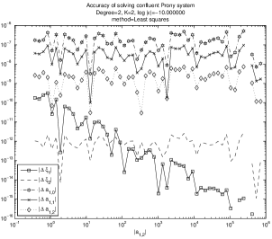
(a) Least squares

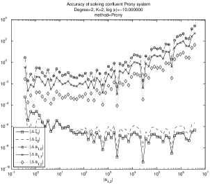
(b) Prony

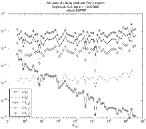
(c) ESPRIT

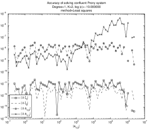
(d) Least squares. Note the growth of $\left|\Delta a_{1,1}\right|$.

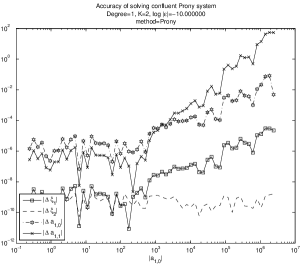
(e) Prony

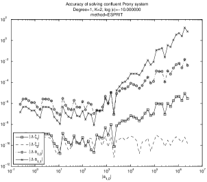
(f) ESPRIT

Figure 1: (a-c): Dependence of the reconstruction error on the magnitude of the highest coefficient, degree = 2.
(d-f): Dependence of the reconstruction error on the magnitude of the “previous” coefficient, degree = 1.

6.B.1 Changing the highest coefficient

In the first set of experiments, we checked how the reconstruction errors $\left|\Delta\xi_{i}\right|,\left|\Delta a_{i,j}\right|$ depend on the magnitude of the highest coefficient $|a_{i,l_{i}-1}|$. The results are presented in Figure 1 on page 1 (a-c).

For both least squares and ESPRIT (but not for Prony), the inverse proportionality $\left|\Delta\xi_{i}\right|\sim\frac{1}{|a_{i,l_{i}-1}|}$ is seen in Figure 1 on page 1 (a), (c), matching the theoretical predictions of Theorem 15.

For LS and ESPRIT, the errors $\left|\Delta a_{i,j}\right|$ seem to be unaffected by the increase in $|a_{i,l_{i}-1}|$. This can be explained very well by the formula $\left|\Delta a_{i,j}\right|\sim 1+\frac{\left|a_{i,j-1}\right|}{\left|a_{i,l_{i}-1}\right|}$ so that indeed $\left|\Delta a_{i,j}\right|$ should remain close to constant as $|a_{i,l_{i}-1}|\to\infty$.

The Prony method’s performance with respect to the recovery of the magnitudes actually degrades with the increase in $|a_{i,l_{i}-1}|$. Although both Prony and ESPRIT use the same method for the recovery of the magnitudes, it appears that the initial error in recovering the nodes, which is significantly smaller in ESPRIT (see Subsection 6.B.3 below), influences this step greatly - in accordance with the predictions of [36, 34] (see also discussion in Subsection 5.C).

In addition, the Prony method fails to separate recovery of a node and its magnitudes (say $\Delta\xi_{1},\Delta a_{1,j}$) from the highest magnitude associated with another node (e.g. $\left|a_{2,l_{2}-1}\right|$) - these results are not shown for saving space.

6.B.2 Changing coefficient other than the highest

In the second set of experiments, we changed the magnitude of some coefficient other than the highest, i.e. $a_{i,j}$ for $j<l_{i}-1$. The results are presented in Figure 1 on page 1 (d-f).

For the least squares method, the dependence of $\left|\Delta a_{i,j}\right|$ on the “previous” magnitude $\left|a_{i,j-1}\right|$ for $j\neq 0$ is consistent with the formula $\left|\Delta a_{i,j}\right|\sim 1+\frac{\left|a_{i,j-1}\right|}{\left|a_{i,l_{i}-1}\right|}$ - such a behavior should be visible when $\left|a_{i,j-1}\right|\gg\left|a_{i,l_{i}-1}\right|$, as can indeed be noticed in Subfigure 1d. In addition, the other magnitudes and the jumps are unaffected, as predicted.

On the contrary, neither Prony nor ESPRIT succeed in confining the influence of $\left|a_{i,j-1}\right|$ only to the recovery of the next magnitude $\left|\Delta a_{i,j}\right|.$ In particular, $\left|\Delta\xi_{1}\right|$ increases with $\left|a_{1,0}\right|$ in both of them. The error in all the magnitudes grows with $\left|a_{1,0}\right|$, as opposed to the least squares where only $\left|\Delta a_{1,1}\right|$ is increased.

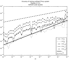
(a) Least squares

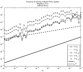
(b) Prony

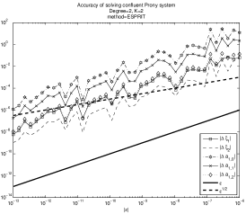
(c) ESPRIT

Figure 2: Reconstruction error as $\varepsilon\to 0$, degree = 2.

6.B.3 Dependence on the measurement error

In the next experiment, we kept all the parameters constant and changed the magnitude of the error $\max_{k}\varepsilon_{k}$. The results are presented in Figure 2 on page 2. The ESPRIT performs slightly better than Prony, but both of them are worse than the optimal least squares. Note however that the asymptotic error (the slope) is $O\left(\varepsilon\right)$ in spite of the fact that both algorithms involve extraction of multiple roots which should decrease the accuracy to $O\left(\varepsilon^{\frac{1}{d}}\right)$ where $d$ is the order of the pole. This phenomenon can be explained by the effect of averaging the clustered roots (see [4, Proposition V.3]).

(a) Least squares

(b) Prony

(c) ESPRIT

Figure 3: Dependence of the reconstruction error on the order of the model.

6.B.4 Dependence on the model order

Next, we checked the dependence of the reconstruction error on the model order $D\stackrel{{\scriptstyle\text{def}}}{{=}}\max_{i=1,\dots,\mathcal{K}}l_{i}.$ The results are presented in Figure 3 on page 3. The reconstruction error for all the parameters grows exponentially in $D$ for all the methods.

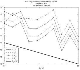
(a) Least squares

(b) Prony

(c) ESPRIT

Figure 4: Dependence of the reconstruction error on the node separation.

6.B.5 Dependence on the node separation

Finally, we checked the dependence of the reconstruction error on the distance between the two nodes $\left|\xi_{2}-\xi_{1}\right|$. The results are presented in Figure 4 on page 4. For all the three methods, the results are consistent with

$$\left|\Delta\xi_{i}\right|,\left|\Delta a_{i,j}\right|\sim\left|\xi_{2}-\xi_{1}\right|^{-D}.$$

6.C Conclusions

In the numerical experiments we have investigated the “best possible local accuracy” via the least squares method, comparing it both with the theoretical results of Theorem 15 and with the performance of two “global” solution techniques, namely Prony and ESPRIT methods, for small perturbations (high SNR). Our results suggest that:

1. The numerical behavior of the solution in the case of small data perturbations indeed exhibits the patterns predicted by Theorem 15, in particular the qualitative dependence of the reconstruction error on the values of the parameters of the problem.

2. The Prony solution method largely fails to separate the parameters which could be separated in theory. Furthermore, its performance actually degrades when the highest coefficient $\left|a_{i,l_{i}-1}\right|$ is increased. ESPRIT separates the parameters better than Prony, but is still worse than optimal.

3. In terms of absolute reconstruction error, ESPRIT is better than Prony but still worse than the optimal LS.

4. In terms of dependence of the reconstruction error on the model order and the node separation, both Prony and ESPRIT behave close to the predicted law, namely exponential increase in the order and polynomial increase in the separation distance.

7 Discussion

We believe that the analytically approach of this paper has the potential to provide relatively complete answer to several important questions related to stable solution of Prony-type systems, as briefly discussed below.

The numerical experiments suggest that the least squares method approximates the optimal “local” behavior very well. However, it is well-known that a very accurate initial approximation is required in order to find the global minima. It is customary to use one of the global solution methods to obtain such an initial value. Further analysis of the Prony sets $\mathcal{M}_{R,S}$ may provide explicit conditions for such an initialization to be sufficiently close to the true solution.

The general case $S\geq R$ should be well-understood in order to estimate the feasibility of taking more measurements than strictly needed (oversampling). Without assumptions on the noise, it is not a-priori obvious that averaging should improve the accuracy in any way. Again, such an understanding is hopefully achievable via the investigation of $\mathcal{M}_{R,S}$ with $S\gg R$.

In practice it is often the case that neither the number of nodes $\mathcal{K}$ nor the numbers $\left\{l_{i}\right\}$ are known a-priori, but only their upper bounds. In this case, given a noisy measurement vector, more than one “explanation” is possible for this data, in which case a good reconstruction algorithm needs somehow to select the “optimal” configuration. One possible way to achieve this goal is to characterize, for each configuration of the system (i.e. $\left\{\mathcal{K},\left\{l_{i}\right\}_{i=1}^{\mathcal{K}}\right\}$), the “stable regions” of the corresponding measurement sets $\mathcal{M}_{R,S}$, for which the accuracy function $\mathcal{ACC}$ does not exceed a predefined upper bound. Based on the initial measurement $\tilde{{\boldsymbol{y}}}\in\mathbb{C}^{S}$ and the error bound $\varepsilon$, an algorithm would choose the closest “stable measurement set”, i.e. select a configuration for which the local accuracy is optimal. Using this approach, collision of two nodes $\xi_{i}$, $\xi_{j}$ can in principle be handled in a stable way by substituting the configuration $\left\{\mathcal{K},\left\{l_{i}\right\}_{i=1}^{\mathcal{K}}\right\}$ with $\left\{\mathcal{K}-1,\left\{l_{1},\dots,l_{i}+l_{j},\dots,l_{\mathcal{K}}\right\}\right\}$ once the measurement vector leaves the stability region associated with the former configuration. In this regard, we note that such a singular behavior has been studied in [48] (see also [33]), where it is shown that if the solution is represented in the basis of divided differences, then the inverse operator is uniformly bounded with respect to the corresponding expansion coefficients. Analogous developments for extraction of multiple roots of polynomials [49] might be very relevant as well.

In order to achieve the above goals, we propose to compute the function $\mathcal{ACC}$ as accurately as possible. For that purpose, more detailed analysis of the Prony map is necessary. In particular, its essential nonlinearity should be quantified using the second-order terms in the Taylor expansion.

In addition to (5), other generalizations of the basic Prony system (1) appear in applications. One such extension arises in Eckhoff’s method [21] for reconstructing piecewise smooth functions from Fourier coefficients. There, an additional parameter appears: namely, the measurements $m_{k}$ are given starting from some large index $k=M$. In [11], we have presented an algorithm for solving this system with high accuracy (in the sense of asymptotic rate of convergence as $M\to\infty$.) However, the question of “maximal possible accuracy” for this problem is still open. It will be most desirable to reinterpret those results in the sense of global stability bounds for Prony-like systems.

References

- [1] B. Adcock, Convergence acceleration of modified Fourier series in one or more dimensions, Mathematics of Computation, 80 (2010), pp. 225–261.
- [2] V. Arnol’d, Hyperbolic polynomials and Vandermonde mappings, Functional Analysis and Its Applications, 20 (1986), pp. 125–127.
- [3] J. Auton, Investigation of Procedures for Automatic Resonance Extraction from Noisy Transient Electromagnetics Data. Volume III. Translation of Prony’s Original Paper and Bibliography of Prony’s Method, tech. rep., Effects Technology Inc., Santa Barbara, CA, 1981.
- [4] R. Badeau, B. David, and G. Richard, High-resolution spectral analysis of mixtures of complex exponentials modulated by polynomials, Signal Processing, IEEE Transactions on, 54 (2006), pp. 1341–1350.
- [5] , Cramér–Rao Bounds for Multiple Poles and Coefficients of Quasi-Polynomials in Colored Noise, Signal Processing, IEEE Transactions on, 56 (2008), pp. 3458–3467.
- [6] , Performance of ESPRIT for estimating mixtures of complex exponentials modulated by polynomials, Signal Processing, IEEE Transactions on, 56 (2008), pp. 492–504.
- [7] N. Banerjee and J. Geer, Exponentially accurate approximations to periodic Lipschitz functions based on Fourier series partial sums, Journal of Scientific Computing, 13 (1998), pp. 419–460.
- [8] D. Batenkov, Moment inversion problem for piecewise D-finite functions, Inverse Problems, 25 (2009), p. 105001.
- [9] D. Batenkov, V. Golubyatnikov, and Y. Yomdin, On one nonlinear problem of reconstructing a planar region with singular boundaries from a finite number of measurements (in Russian), Department of Mathematical Analysis, Gorno-Altayskiy Univ., Russia, 2 (2010), pp. 17 – 23.
- [10] , Reconstruction of Planar Domains from Partial Integral Measurements, in Proc. Complex Analysis & Dynamical Systems V, 2011.
- [11] D. Batenkov and Y. Yomdin, Algebraic Fourier reconstruction of piecewise smooth functions, Mathematics of Computation, 81 (2012), pp. 277–318.
- [12] F. Bazán, Conditioning of rectangular Vandermonde matrices with nodes in the unit disk, SIAM Journal on Matrix Analysis and Applications, 21 (2000), p. 679.
- [13] B. Beckermann, The condition number of real Vandermonde, Krylov and positive definite Hankel matrices, Numerische Mathematik, 85 (2000), pp. 553–577.
- [14] B. Beckermann, A. Matos, and F. Wielonsky, Reduction of the Gibbs phenomenon for smooth functions with jumps by the -algorithm, Journal of Computational and Applied Mathematics, 219 (2008), pp. 329–349.
- [15] Z. Ben-Haim, T. Michaeli, and Y. Eldar, Performance bounds for the estimation of finite rate of innovation signals from noisy measurements, in Sensor Array and Multichannel Signal Processing Workshop (SAM), 2010 IEEE, 2010, pp. 97 –100.
- [16] Å. Björck and T. Elfving, Algorithms for confluent Vandermonde systems, Numerische Mathematik, 21 (1973), pp. 130–137.
- [17] D. Boley, F. Luk, and D. Vandevoorde, Vandermonde factorization of a Hankel matrix, in Scientific Computing: Proceedings of the Workshop, 10-12 March 1997, Hong Kong, Springer, 1998, p. 27.
- [18] E. Candes and C. Fernandez-Granda, Towards a mathematical theory of super-resolution, Arxiv preprint arXiv:1203.5871, (2012).
- [19] P. Dragotti, M. Vetterli, and T. Blu, Sampling Moments and Reconstructing Signals of Finite Rate of Innovation: Shannon meets Strang-Fix, IEEE Transactions on Signal Processing, 55 (2007), p. 1741.
- [20] T. Driscoll and B. Fornberg, A Padé-based algorithm for overcoming the Gibbs phenomenon, Numerical Algorithms, 26 (2001), pp. 77–92.
- [21] K. Eckhoff, Accurate reconstructions of functions of finite regularity from truncated Fourier series expansions, Mathematics of Computation, 64 (1995), pp. 671–690.
- [22] W. Gautschi, On inverses of Vandermonde and confluent Vandermonde matrices, Numerische Mathematik, 4 (1962), pp. 117–123.
- [23] G. Golub, P. Milanfar, and J. Varah, A Stable Numerical Method for Inverting Shape from Moments, SIAM Journal on Scientific Computing, 21 (2000), pp. 1222–1243.
- [24] B. Gustafsson, C. He, P. Milanfar, and M. Putinar, Reconstructing planar domains from their moments, Inverse Problems, 16 (2000), pp. 1053–1070.
- [25] K. Holmström and J. Petersson, A review of the parameter estimation problem of fitting positive exponential sums to empirical data, Applied Mathematics and Computation, 126 (2002), pp. 31 – 61.
- [26] M. Kahn, M. Mackisack, M. Osborne, and G. Smyth, On the consistency of Prony’s method and related algorithms, Journal of Computational and Graphical Statistics, (1992), pp. 329–349.
- [27] S. Kay, Fundamentals of Statistical Signal Processing, 1993, Prentice-Hall, 1993.
- [28] G. Kvernadze, Approximating the jump discontinuities of a function by its Fourier-Jacobi coefficients, Mathematics of Computation, 73 (2004), pp. 731–752.
- [29] H. Lu, Fast Solution of Confluent Vandermonde Linear Systems, SIAM J. Matrix Anal. Appl., 15 (1994), pp. 1277–1289.
- [30] L. S. Maergoîz, A multidimensional version of prony’s algorithm, Siberian Mathematical Journal, 35 (1994), pp. 351–366. 10.1007/BF02104782.
- [31] I. Maravic and M. Vetterli, Sampling and reconstruction of signals with finite rate of innovation in the presence of noise, IEEE Transactions on Signal Processing, 53 (2005), pp. 2788–2805.
- [32] R. March and P. Barone, Application of the Pade method to solve the noisy trigonometric moment problem: some initial results, SIAM J. Appl. Math, 58 (1998), pp. 324–343.
- [33] M. Osborne, Some special nonlinear least squares problems, SIAM Journal on Numerical Analysis, 12 (1975), pp. 571–592.
- [34] T. Peter, D. Potts, and M. Tasche, Nonlinear approximation by sums of exponentials and translates, SIAM Journal on Scientific Computing, 33 (2011), p. 1920.
- [35] A. Poghosyan, Asymptotic behavior of the Eckhoff method for convergence acceleration of trigonometric interpolation, Analysis in Theory and Applications, 26 (2010), pp. 236–260.
- [36] D. Potts and M. Tasche, Parameter estimation for exponential sums by approximate Prony method, Signal Processing, 90 (2010), pp. 1631–1642.
- [37] R. Prony, Essai experimental et analytique, J. Ec. Polytech.(Paris), 2 (1795), pp. 24–76.
- [38] B. Rao and K. Arun, Model based processing of signals: A state space approach, Proceedings of the IEEE, 80 (1992), pp. 283–309.
- [39] N. Sarig and Y. Yomdin, Signal Acquisition from Measurements via Non-Linear Models, Mathematical Reports of the Academy of Science of the Royal Society of Canada, 29 (2008), pp. 97–114.
- [40] L. Schumaker, Spline functions: basic theory, (1981).
- [41] H. So and K. Chan, New insights on Pisarenko’s method for sinusoidal frequency estimation, in Signal Processing and Its Applications, 2003. Proceedings. Seventh International Symposium on, vol. 2, IEEE, 2003, pp. 503–506.
- [42] P. Stoica and N. Arye, MUSIC, maximum likelihood, and Cramer-Rao bound, IEEE Transactions on Acoustics, Speech and Signal Processing, 37 (1989), pp. 720–741.
- [43] P. Stoica and R. Moses, Spectral analysis of signals, Pearson/Prentice Hall, 2005.
- [44] J. Urigüen, P. Dragotti, and T. Blu, On the exponential reproducing kernels for sampling signals with finite rate of innovation, in Proc. of Sampling Theory and Application Conference, Singapore, 2011.
- [45] M. VanBlaricum and R. Mittra, Problems and solutions associated with Prony’s method for processing transient data, IEEE Transactions on Antennas and Propagation, 26 (1978), pp. 174–182.
- [46] M. Vetterli, P. Marziliano, and T. Blu, Sampling signals with finite rate of innovation, IEEE Transactions on Signal Processing, 50 (2002), pp. 1417–1428.
- [47] J. Wilkinson, Rounding errors in algebraic processes, Dover Pubns, 1994.
- [48] Y. Yomdin, Singularities in Algebraic Data Acquisition, in Real and Complex Singularities, M. Manoel, M. Fuster, and C. Wall, eds., Cambridge University Press, 2010.
- [49] Z. Zeng, Computing multiple roots of inexact polynomials, Mathematics of Computation, 74 (2005), pp. 869–904.