DCPT-11/23
Broken Baby Skyrmions

Abstract

The baby Skyrme model is a (2+1)-dimensional analogue of the Skyrme model, in which baryons are described by topological solitons. In this paper we introduce a version of the baby Skyrme model in which the global $O(3)$ symmetry is broken to the dihedral group $D_{N}.$ It is found that the single soliton in this theory is composed of $N$ partons, that are topologically confined. The case $N=3$ is studied in some detail and multi-soliton solutions are computed. These soliton solutions are related to polyiamonds, which are plane figures composed of equilateral triangles joined by common edges. It is shown that the solitons may be viewed as pieces of a doubly periodic soliton lattice. An alternative model with $D_{3}$ symmetry is also introduced, which has an exact explicit soliton lattice solution. Soliton solutions are computed and compared in the two $D_{3}$ theories. Some comments are made regarding the extension of these ideas to the Skyrme model.

1 Introduction

The Skyrme model [1] is a nonlinear field theory in which baryons are described by topological solitons, called Skyrmions. The model has been obtained from quantum chromodynamics (QCD) as a low energy effective field theory in the limit in which the number of colours, $N,$ is large [2]. More recently, the Skyrme model has been derived from string theory, in the context of holographic QCD, again in the large $N$ limit [3].

The number of colours, $N,$ appears in the Skyrme model only as a coefficient of the Wess-Zumino term. This plays an important role in the quantization of Skyrmions, but at the classical level the soliton solutions are blind to the value of $N;$ as the Wess-Zumino term does not contribute to the classical energy. An interesting issue is whether it is possible to incorporate an effective small value of $N$ at the level of the classical soliton solution.

The baby Skyrme model [4] is a (2+1)-dimensional analogue of the Skyrme model, that has proved to be a useful testing ground for the study of Skyrmions. Soliton solutions of the baby Skyrme and related models are also of interest in their own right, within the context of condensed matter physics [5, 6], where direct experimental observations can be made.

In this paper we introduce a version of the baby Skyrme model in which the global $O(3)$ symmetry is broken to the dihedral group $D_{N}.$ It is shown that this reproduces some key features expected of Skyrmions in a toy model associated with a small number of colours. In particular, it is found that the single soliton in this theory is composed of $N$ partons, that are topologically confined. The case $N=3$ is studied in some detail and multi-soliton solutions are computed. The model admits a variety of stable multi-solitons that take the form of polyiamonds; which are plane figures composed of equilateral triangles joined by common edges. Doubly periodic soliton lattices are also computed and it is shown that the polyiamond solitons may be viewed as pieces of a soliton lattice.

An alternative model with $D_{3}$ symmetry is also introduced and studied. This model has the property that an exact soliton lattice solution is given explicitly in terms of a Weierstrass elliptic function. Soliton solutions are computed and compared in the two $D_{3}$ theories.

2 The broken baby Skyrme model

The field of the baby Skyrme model is a three-component unit vector ${\mbox{\boldmath$\phi$}}=(\phi_{1},\phi_{2},\phi_{3}).$ In this paper we are concerned with static solitons, hence the theory may be defined by its static energy, which takes the form

$$E=\int\bigg{(}\frac{1}{2}\partial_{i}\mbox{\boldmath$\phi$}\cdot\partial_{i}\mbox{\boldmath$\phi$}+\frac{\kappa^{2}}{4}(\partial_{i}\mbox{\boldmath$\phi$}\times\partial_{j}\mbox{\boldmath$\phi$})\cdot(\partial_{i}\mbox{\boldmath$\phi$}\times\partial_{j}\mbox{\boldmath$\phi$})+V\bigg{)}\,d^{2}x,$$ (2.1)

where $V(\mbox{\boldmath$\phi$})$ is a potential and $\kappa$ is a constant. In the standard baby Skyrme model [4] the potential is taken to be

$$V=m^{2}(1-\phi_{3}),$$ (2.2)

which is the analogue of the conventional pion mass term in the Skyrme model [7]. The constant $m$ gives the mass of the fields $\phi_{1}$ and $\phi_{2},$ associated with elementary excitations around the unique vacuum $\mbox{\boldmath$\phi$}=(0,0,1).$

Finite energy requires that the field takes the vacuum value at all points at spatial infinity, $\mbox{\boldmath$\phi$}(\infty)=(0,0,1).$ This compactification means that topologically $\phi$ is a map between two-spheres, with an associated integer winding number $B\in\hbox{\mybb Z}=\pi_{2}(S^{2}).$ This topological charge (or soliton number) is the analogue of the baryon number in the Skyrme model and may be calculated as

$$B=-\frac{1}{4\pi}\int\mbox{\boldmath$\phi$}\cdot(\partial_{1}\mbox{\boldmath$\phi$}\times\partial_{2}\mbox{\boldmath$\phi$})\,d^{2}x.$$ (2.3)

An application of Derrick’s theorem [8] reveals that the scale of a soliton in the baby Skyrme model is determined by the ratio $\sqrt{\kappa/m}.$

The first two terms in the energy (2.1) are invariant under the global $O(3)$ symmetry, $\mbox{\boldmath$\phi$}\mapsto{\cal O}\mbox{\boldmath$\phi$}$ for ${\cal O}\in O(3),$ but this is broken by the potential (2.2) to an $O(2)$ symmetry acting on the first two components $\phi_{1},\phi_{2}.$ The single soliton takes advantage of this symmetry and is axially symmetric [4].

Other choices for the potential have been investigated [9, 10], but in these examples there is an unbroken $O(2)$ symmetry and the $B=1$ soliton is axially symmetric. A novel situation was considered recently [11] using the easy plane potential $V=\frac{1}{2}m^{2}\phi_{1}^{2}.$ Again this leaves an unbroken $O(2)$ symmetry, but in this case the choice of a vacuum value at spatial infinity, for example $\mbox{\boldmath$\phi$}(\infty)=(0,0,1),$ distinguishes a point on the orbit of the unbroken symmetry and further breaks the symmetry to the dihedral group $D_{2}.$ In this case the single soliton is not axially symmetric, but turns out to be composed of two constituents. The work on easy plane baby Skyrmions provided some inspiration for the model proposed in the current paper, but it should be stressed that the two theories are quite different, as described shortly.

The only previous work we are aware of in which the potential has only a discrete symmetry is the work of Ward [12], in which the symmetry is broken to the dihedral group $D_{2}$ by the choice $V=\frac{1}{2}m^{2}(1-\phi_{3}^{2})(1-\phi_{1}^{2}).$ In this theory the single soliton is also composed of two constituents. We shall discuss this theory in more detail in section 5, where we introduce a generalization to a model with $D_{3}$ symmetry and compare the results with those obtained for the theory of main concern in this paper.

The theory introduced in the present paper has the potential

$$V=m^{2}\,|1-(\phi_{1}+i\phi_{2})^{N}|^{2}\,(1-\phi_{3}),$$ (2.4)

where $N\geq 2$ is an integer parameter of the model. We shall refer to the theory with this potential as the broken baby Skyrme model with $N$ colours, to use a suggestive notation. The global $O(3)$ symmetry is broken by this potential to the dihedral group $D_{N},$ generated by the rotation $(\phi_{1}+i\phi_{2})\mapsto(\phi_{1}+i\phi_{2})e^{i2\pi/N}$ and the reflection $(\phi_{1},\phi_{2},\phi_{3})\mapsto(\phi_{1},-\phi_{2},\phi_{3}).$ In the context of symmetry groups in three dimensions, this pyramidal symmetry group is often denoted $C_{Nv},$ but as an abstract group it is isomorphic to $D_{N},$ which is a more convenient notation for the later application to planar symmetries.

The potential (2.4) has $N+1$ vacua on the two-sphere. The vacuum at the north pole $\mbox{\boldmath$\phi$}=(0,0,1),$ will be the chosen vacuum at spatial infinity, with the remaining $N$ vacua lying on the equatorial circle $\phi_{3}=0$ at the $N$th roots of unity. Note that this choice of boundary condition does not break any further symmetries, in contrast to the situation for the easy plane potential. Another important difference between the two theories concerns the masses of the elementary excitations of the fields $\phi_{1}$ and $\phi_{2}.$ To quadratic order in $\phi_{1}$ and $\phi_{2},$ the broken potential (2.4) agrees with the standard baby Skyrme potential (2.2), hence both fields $\phi_{1}$ and $\phi_{2}$ have mass $m.$ However, for the easy plane potential clearly only the $\phi_{1}$ field has mass $m$ and the $\phi_{2}$ field is massless. Hopefully, this brief discussion has served to highlight some of the important differences between the two models, making it clear that different phenomena should be expected, even in the case $N=2$ where both theories have the same unbroken symmetry group $D_{2}.$

Ward’s potential [12] with $D_{2}$ symmetry has more in common with the two colour broken baby Skyrme model, as both fields $\phi_{1}$ and $\phi_{2}$ have the same mass. However, there is an additional inversion symmetry $\mbox{\boldmath$\phi$}\mapsto-\mbox{\boldmath$\phi$},$ with an associated extra vacuum $\mbox{\boldmath$\phi$}=(0,0,-1),$ which leads to some qualitative differences in the soliton solutions.

3 Solitons and polyiamonds

Whether in two or three dimensions, a symmetry of a soliton in a Skyrme model refers to an equivariance in which a spatial rotation or reflection can be compensated by the action of the global symmetry of the theory. Clearly the maximal symmetry possible in the broken baby Skyrme model with $N$ colours is dihedral symmetry $D_{N}.$ Even the $B=1$ single soliton cannot be axially symmetric, though the expectation is that it has the maximal symmetry $D_{N}.$ Numerical solutions presented in this section confirm this expectation and reveal that the single soliton is composed of $N$ constituents, which we refer to as partons, given that in the Skyrme model the single soliton describes the proton.

Each parton carries baryon number $B=1/N,$ associated with a winding that covers this fraction of the target two-sphere. Partons are topologically confined, since finite energy requires that the total baryon number is integer-valued, hence an equal number of partons of each colour. Here the term colour may be used to enumerate the $N$ segments of the target two-sphere obtained by drawing great semi-circles from the north pole to the south pole that pass through each of the $N$ equatorial vacua. Of course a parton and an anti-parton (associated with a winding of the same segment with the opposite orientation) is an allowed combination, corresponding to elementary excitations of the $\phi_{1}$ and $\phi_{2}$ fields with zero baryon number, being the baby Skyrme analogue of pions.

From now on we shall concentrate on the most physically relevant case of $N=3$ colours, regarding the theory as a lower-dimensional analogue of the Skyrme model. The generic values $\kappa=m=1$ are taken for the parameters of the theory.

To numerically construct soliton solutions an energy minimizing gradient flow algorithm is applied to the energy (2.1). Spatial derivatives are approximated using fourth-order accurate finite difference approximations with a lattice spacing $\Delta x=0.05$ and $251^{2}$ grid points. At the boundary of the grid the field is fixed to the vacuum value $\mbox{\boldmath$\phi$}=(0,0,1).$

A field with topological charge $B$ is given by

$$\mbox{\boldmath$\phi$}=(\sin f\cos(B\theta),\sin f\sin(B\theta),\cos f),$$ (3.1)

where $r$ and $\theta$ are polar coordinates in the plane with $f(r)$ any monotonically decreasing radial profile function such that $f(0)=\pi$ and $f$ vanishes at the boundary of the grid.

The field (3.1) has dihedral symmetry $D_{3B},$ with the spatial rotation $\theta\mapsto\theta+2\pi/(3B)$ being compensated by the global transformation $(\phi_{1}+i\phi_{2})\mapsto(\phi_{1}+i\phi_{2})e^{-i2\pi/3},$ and the spatial reflection $\theta\mapsto-\theta$ compensated by the global reflection $(\phi_{1},\phi_{2},\phi_{3})\mapsto(\phi_{1},-\phi_{2},\phi_{3}).$ Note that either a spatial reflection or a global reflection alone changes the sign of the topological charge, but the combination of the two leaves it unchanged.

Using the field (3.1) as an initial condition in the numerical energy minimization code yields a charge $B$ solution with $D_{3B}$ symmetry. The energy density of the $B=1$ soliton is displayed as a contour plot in Figure 1.1, which clearly shows the three constituent partons. A plot of the topological charge density (the integrand in (2.3)) has a similar structure. The energy of this $D_{3}$ symmetric $B=1$ soliton is $E=34.79,$ and is listed in Table 1. For all the numerical results presented in this paper, the topological charge computed using the lattice version of (2.3) is integer-valued to five significant figures, which provides an indication of the accuracy expected in the numerical computations.

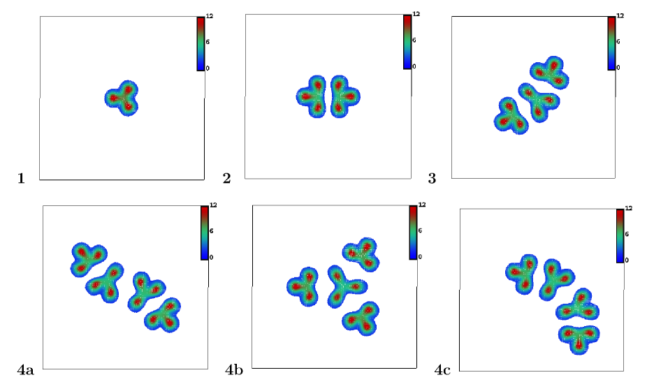
Figure 1: Energy density contour plots for solitons with charge $B.$ The top row displays stable solitons for $B=1,2,3$ and the bottom row shows three different stable solitons with $B=4.$

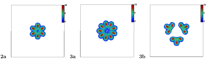
Figure 2: Energy density contour plots for solitons with charge $B.$                           2a) $B=2$ hexagon;  3a) $B=3$ nonagon;  3b) $B=3$ triquetra.

$B$	$E/B$	$G$	Figure
1	34.79	$D_{3}$	1.1
2	33.04	$D_{6}$	2.2a
2	33.06	$D_{2}$	1.2
3	32.83	$D_{1}$	1.3
3	33.00	$D_{3}$	2.3b
3	33.68	$D_{9}$	2.3a
4	32.68	$C_{2}$	1.4a
4	32.70	$D_{1}$	1.4c
4	32.96	$D_{3}$	1.4b

Table 1: The energy per soliton $E/B$ and symmetry group $G$ of solitons with topological charge $B\leq 4.$

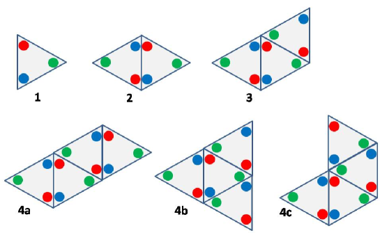
Figure 3: The six possible polyiamonds constructed from at most four triangles.

The $D_{3B}$ symmetric solution is composed of $3B$ partons located at the vertices of a regular $3B$-gon. The solutions with $B=2$ and $B=3$ are displayed in Figures 2.2a and  2.3a respectively. For $B>2$ such solutions are unstable to perturbations that break the dihedral symmetry. The $B=2$ hexagonal solution is stable with an energy per soliton of $E/B=33.04.$ A sufficiently large symmetry breaking perturbation can convert this solution into the additional stable $D_{2}$ symmetric soliton displayed in Figure 1.2. The energy per soliton of this solution is $E/B=33.06,$ so the two different $B=2$ solutions have energies that differ by an amount comparable to our expected numerical accuracy, and we are unable to make a confident statement about which has the lower energy. It is clear from Figure 1.2 that this $B=2$ soliton is constructed from two $B=1$ solitons, with a relative spatial rotation of $180^{\circ}.$

As mentioned earlier, the asymptotic fields of a soliton in the broken baby Skyrme model have the same form as those in the standard baby Skyrme model; hence the results on asymptotic interactions derived in [4] can be transfered to the current theory (see Appendix A for a discussion of asymptotic forces for a general potential). In particular, the leading order result shows that two single solitons are maximally attractive if one is rotated relative to the other through an angle of $180^{\circ}.$ As the single soliton in the broken baby Skyrme model is not axially symmetric, then beyond leading order there will be a contribution that differentiates between the relative orientation of the two triangles of partons. The result presented in Figure 1.2 displays the optimal orientation between the two triangles, which can be confirmed by using an initial condition consisting of two well-separated single solitons with a generic initial orientation.

It is instructive to represent the single soliton, as in Figure 3.1, as a triangle with three coloured dots to denote the three peaks in the energy density associated with the three segments of the target two-sphere. With this representation the $B=2$ soliton in Figure 1.2 corresponds to the diamond in Figure 3.2, in which the two triangles share a common edge with adjacent dots being different colours.

This triangle representation suggests that multi-solitons will correspond to polyiamonds. A polyiamond [13] is a plane figure composed of identical equilateral triangles joined by common edges, so that no two triangles overlap. For three triangles there is a unique triamond, shown in Figure 3.3. Given a polyiamond, and a colour assignment to any one of the triangles, there is a unique colouring of the triangles satisfying the rule of different adjacent colours.

The initial condition (3.1) with $B=3$ yields the unstable $D_{9}$ symmetric nonagon displayed in Figure 2.3a with an energy per soliton of $E/B=33.68.$ A symmetry breaking perturbation leads to the $B=3$ soliton displayed in Figure 1.3 with $E/B=32.83.$ This confirms the predicted triamond form of Figure 3.3, which has only a reflection symmetry, $D_{1},$ and no rotational symmetry. This $B=3$ soliton can also be obtained from an initial condition consisting of three well-separated single solitons with appropriate positions and orientations. A stable $B=3$ local energy minimum has also been computed that is not of the polyiamond form. It has an energy per soliton of $E/B=33.00$ and is presented in Figure 2.3b. This triquetra solution has $D_{3}$ symmetry and is formed from three triangles that share vertices but not edges.

With four triangles there are the three tetriamonds shown in Figures 3.4a, 3.4b and 3.4c. Suitable initial conditions, using four well-separated single solitons with appropriate positions and orientations, leads to $B=4$ solitons associated with each of these tetriamonds. Energy density plots for all three solitons are displayed in the bottom row of Figure 1 and the associated energies are listed in Table 1. All three solutions appear to be stable and their energies are very close to each other. This can be understood from the fact that all pairs of triangles that share a common edge are in a maximally attractive orientation. Furthermore, to transform from one configuration to another requires the breaking of an attractive bond followed by a change of orientation and a repositioning of a triangle.

The number of polyiamonds grows rapidly with the number of triangles, and the expectation is that there will be a soliton associated with each of these. There are five pentiamonds (including the first asymmetric configuration with neither a rotation nor a reflection symmetry) and twelve hexiamonds. Already for $B=9$ there are 160 polyiamonds, so it is likely to be a computationally intensive task to numerically compute all the solitons for values of $B$ larger than those considered in this paper. However, it could be a worthwhile exercise that might lead to an interesting energy function on the space of polyiamonds. Based on the result for $B=4,$ it could be that the linear arrangement of triangles is minimal for all values of $B.$ This would have some similarities with the standard baby Skyrme model, where soliton chains are found to be the minimal energy configurations [14].

Note that the $B=3$ triquetra solution in Figure 2.3b is related to the $B=4$ tetriamond solution in Figure 1.4b by removing the central triangle. A local energy minimum with $B=4$ has been computed that is not of the polyiamond form but is related to the triquetra solution by the addition of a triangle (in the polyiamond manner) on an outside edge of the triquetra, rather than in the middle. It is expected that a variety of similar local energy minima exist for all $B\geq 4,$ based on extending the triquetra solution in this manner.

4 Soliton lattices

The polyiamond solutions in Figure 1 suggest the existence of a doubly periodic triangular lattice, associated with a tiling of the plane by equalateral triangles. To study a lattice with triangular symmetry it is sufficient to restrict to the fundamental torus $\hbox{\mybb T}^{2}$ with a $60^{\circ}$ angle in the $(x_{1},x_{2})$ plane. It is useful to note that several identities may be derived for such a lattice to be a critical point of the energy (2.1) (see Appendix B).

The first identity is a standard virial relation that follows from an application of Derrick’s theorem [8] and is a requirement of criticality under a rescaling of the lattice

$$\int_{\hbox{\mybb T}^{2}}\bigg{(}\frac{\kappa^{2}}{4}(\partial_{i}\mbox{\boldmath$\phi$}\times\partial_{j}\mbox{\boldmath$\phi$})\cdot(\partial_{i}\mbox{\boldmath$\phi$}\times\partial_{j}\mbox{\boldmath$\phi$})-V\bigg{)}\,d^{2}x=0.$$ (4.2)

The two remaining identities follow from variations of the lattice associated with a stretch of one of the fundamental periods and a variation of the angle of the fundamental torus from $60^{\circ}$

$$\int_{\hbox{\mybb T}^{2}}\bigg{(}\partial_{1}\mbox{\boldmath$\phi$}\cdot\partial_{1}\mbox{\boldmath$\phi$}-\partial_{2}\mbox{\boldmath$\phi$}\cdot\partial_{2}\mbox{\boldmath$\phi$}\bigg{)}\,d^{2}x=0,$$ (4.3)

and

$$\int_{\hbox{\mybb T}^{2}}\partial_{1}\mbox{\boldmath$\phi$}\cdot\partial_{2}\mbox{\boldmath$\phi$}\ d^{2}x=0.$$ (4.4)

For computational purposes it is convenient to work with a rectangular torus of the form $(x_{1},x_{2})\in[0,L]\times[0,\sqrt{3}L],$ containing two copies of the fundamental torus. Numerical simulations can then be performed in the rectangular torus with periodic boundary conditions in both the $x_{1}$ and $x_{2}$ directions. An initial value is chosen for the length $L$ of the torus and the energy minimized using the numerical methods described in the previous section. The virial relation (4.2) is then evaluated and used to predict an improved estimate for the torus length $L.$ This procedure is iterated to convergence and finally the two remaining identities (4.3) and (4.4) are checked. For the results presented in this paper the rectangular lattice contains $52\times 90$ grid points and all three identities are satisfied to an accuracy of better than $1\%.$

The fundamental torus of a triangular tiling contains two triangles, hence the rectangular torus contains a field with topological charge $B=4.$ An initial condition is provided by setting $B=4$ in the ansatz (3.1) and using a radial profile function with a compact support inside the rectangular torus. A periodic perturbation is applied to this initial condition, to break any reflection symmetries. The result of the numerical minimization is displayed in the left-hand side of Figure 4. The minimizing torus length is $L=5.38,$ with an energy per soliton for this lattice equal to $E/B=31.83.$ This value is consistent as a limit of the finite $B$ polyiamond energies presented in Table 1.

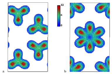
Figure 4: Energy density contour plots for two different soliton lattices. On the left is a triangular lattice of single solitons and on the right is a hexagonal lattice of double solitons. The single soliton lattice has a slightly lower energy per soliton.

There is a second soliton lattice, based on the hexagonal $B=2$ soliton of Figure 2.2a. This lattice is obtained if the initial condition is not subjected to a perturbation that breaks the left-right reflection symmetry. This lattice is displayed in the right-hand side of Figure 4. In this case the minimizing torus length is slightly reduced at $L=5.10$ and the energy per soliton is a little greater at $E/B=32.43.$ The fact that the energy of the double soliton lattice is larger than that of the single soliton lattice agrees with the preferred polyiamond form of the minimal energy solitons with $B>2.$

All the polyiamond solutions in Figure 1 may be viewed as finite $B$ pieces cut from the soliton lattice presented in the left-hand side of Figure 4. This explains why different solutions with the same value of $B$ have very similar energies. The difference is an edge effect associated with the way in which a finite $B$ piece is cut from the infinite lattice. This supports the expectation that stable soliton solutions exist for each polyiamond and suggests that the energy differences between solutions will decrease as $B$ increases.

5 An alternative $D_{3}$ model

As mentioned earlier, in [12] Ward introduced a potential with $D_{2}$ symmetry. It has the novel feature that an exact explicit solution exists for the soliton lattice, with the single soliton composed of two partons. The lattice has square symmetry and consists of half solitons. In this section, we apply Ward’s analysis to construct a potential with $D_{3}$ symmetry, for which there is an exact explicit triangular lattice solution. We then investigate the solitons of this alternative $D_{3}$ model, pointing out some of the differences and similarities with our earlier three colour theory.

Consider the energy (2.1) defined on a torus $\hbox{\mybb T}^{2},$ with an arbitrary potential $V.$ Let $b$ denote the topological charge density, the integrand in (2.3),

$$b=-\frac{1}{4\pi}\mbox{\boldmath$\phi$}\cdot(\partial_{1}\mbox{\boldmath$\phi$}\times\partial_{2}\mbox{\boldmath$\phi$}).$$ (5.1)

The inequality

$$(4\pi\kappa b-\sqrt{2V})^{2}\geq 0$$ (5.2)

leads to the following lower bound for the energy on the torus

$$E\geq 4\pi\bigg{(}B+\kappa\int_{\hbox{\mybb T}^{2}}b\sqrt{2V}\,d^{2}x\bigg{)},$$ (5.3)

where, without loss of generality, we have restricted to the situation where $B>0.$

Following [12], the inequality (5.3) can be written as a Bogomolny bound

$$E/B\geq 4\pi+\kappa\beta,$$ (5.4)

where $\beta$ is the constant

$$\beta=\int_{S^{2}}\sqrt{2V}\,d^{2}S,$$ (5.5)

with $d^{2}S$ the standard area element on the target two-sphere, normalized to $4\pi.$

To investigate the bound further, it is useful to introduce complex coordinates on both the domain and target by defining $z=x_{1}+ix_{2}$ and $W=(\phi_{1}+i\phi_{2})/(1-\phi_{3}).$ A necessary condition to attain the bound (5.4) is that $W$ is a meromorphic function of $z.$ With this assumption the topological charge density (5.1) becomes

$$b=\frac{1}{\pi(1+|W|^{2})^{2}}\bigg{|}\frac{dW}{dz}\bigg{|}^{2}.$$ (5.6)

The bound is then attained if the inequality (5.2) becomes an equality, which requires

$$V=\frac{8\kappa^{2}}{(1+|W|^{2})^{4}}\bigg{|}\frac{dW}{dz}\bigg{|}^{4}.$$ (5.7)

This defines a suitable potential if $dW/dz$ is an explicit function of $W.$ As the domain is a torus, the most elegant choice is to take $W$ to be proportional to a Weierstrass elliptic function. For simplicity, we set $W(z)=\wp(z),$ where the Weierstrass function is defined in terms of the invariants $g_{2},g_{3}$ by

$$\bigg{(}\frac{d\wp}{dz}\bigg{)}^{2}=4\wp^{3}-g_{2}\wp-g_{3}.$$ (5.8)

Substituting this choice into (5.7) yields the family of potentials

$$V=\frac{8\kappa^{2}|4W^{3}-g_{2}W-g_{3}|^{2}}{(1+|W|^{2})^{4}}.$$ (5.9)

Ward studied the case $g_{3}=0,$ when the potential (5.9) has $D_{2}$ symmetry ($W\mapsto iW$), with an exact lattice solution of half solitons and square symmetry [12]. In this paper we consider the theory with $g_{2}=0,$ so that there is $D_{3}$ symmetry ($W\mapsto e^{i2\pi/3}W$). Different values of $g_{3}$ are related by a scaling symmetry, which we use to set $g_{3}=4.$ The potential of our alternative $D_{3}$ model is therefore given by

$$V=\frac{128\kappa^{2}|1-W^{3}|^{2}}{(1+|W|^{2})^{4}}=16\kappa^{2}(1-\phi_{3})(1+3\phi_{3}^{2}+3\phi_{1}\phi_{2}^{2}-\phi_{1}^{3}),$$ (5.10)

where in the final expression the potential is written in terms of the field $\mbox{\boldmath$\phi$}.$

As in the previous sections, from now on we set $\kappa=1.$ The vacua of the potential (5.10) are the same as those of the three colour broken baby Skyrme model (2.4). Considering elementary excitations around the vacuum $\mbox{\boldmath$\phi$}=(0,0,1),$ reveals that the fields $\phi_{1}$ and $\phi_{2}$ both have mass $m=8.$ This is not an important difference, and is simply a consequence of our choice of scaling for the exact elliptic function solution, but does mean that the scale of the solitons will be smaller in the alternative $D_{3}$ model and the energies higher.

A significant difference between the two $D_{3}$ theories concerns the relative values of the potential at particular points of interest on the target two-sphere. These four points are $\mbox{\boldmath$\phi$}=(0,0,-1),$ defining the centre of the soliton, and the three points on the equator midway between the equatorial vacua, such as $\mbox{\boldmath$\phi$}=(-1,0,0).$ In the broken baby Skyrme model the potential at a midway point is greater than the potential at the soliton centre, producing a split of the single soliton energy density into three peaks. However, for the alternative $D_{3}$ theory this situation is reversed, so the energy density is not split but is simply stretched into a triangular deformation. In this sense the alternative model does not reveal the parton constituents in the same way as the broken baby Skyrme model. However, as we now describe, there are a number of similarities between the solitons of the two theories.

The energy density of the exact elliptic function solution is displayed in Figure 5. To aid comparison with the previous lattice solutions, the energy density is plotted for a rectangular torus containing two copies of the fundamental torus. The length of the rectangular torus is equal to the real period of the elliptic function, hence $L=\omega_{1}=\Gamma(\frac{1}{6})\Gamma(\frac{1}{3})/(2\sqrt{3\pi})=2.428...$

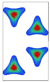
Figure 5: An energy density contour plot of the lattice of single solitons given by an exact elliptic function solution of the alternative $D_{3}$ model.

A numerical evaluation of the integral (5.5) yields $\beta=89.30$ and hence from (5.4) an energy per soliton of $E/B=101.86.$ Note the similarity between Figure 5 and the left-hand side of Figure 4. Both are triangular lattices of single solitons, with the main difference being that the energy density of the single soliton is not split into three peaks in the alternative $D_{3}$ theory, as discussed above. The similarity between the minimal energy lattices in the two theories suggests that solitons in the alternative $D_{3}$ theory may also be related to polyiamonds. To investigate this issue, the same numerical code used in section 3 is applied to the problem, with the only change being a reduction in the lattice spacing to $\Delta x=0.02,$ reflecting the smaller scale of the solitons.

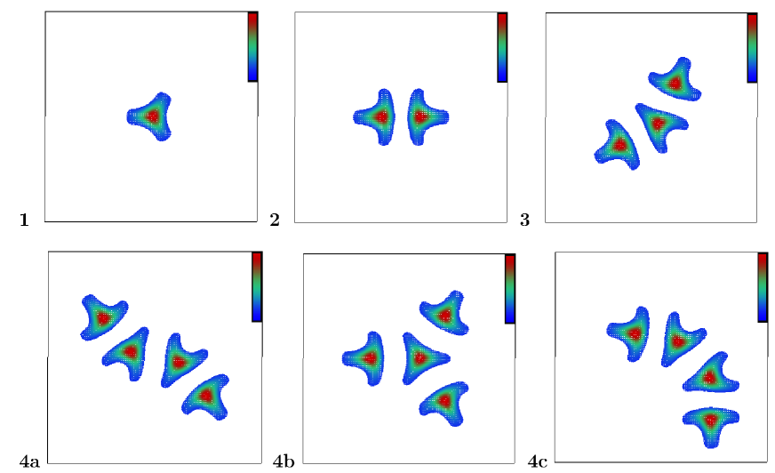
Figure 6: Energy density contour plots for solitons of charge $B$ in the alternative $D_{3}$ model. The top row displays stable solitons for $B=1,2,3$ and the bottom row shows three different stable solitons with $B=4.$

$B$	$E/B$	$G$	Figure
1	108.99	$D_{3}$	6.1
2	105.80	$D_{2}$	6.2
3	104.99	$D_{1}$	6.3
4	104.59	$C_{2}$	6.4a
4	104.62	$D_{1}$	6.4c
4	104.81	$D_{3}$	6.4b

Table 2: The energy per soliton $E/B$ and symmetry group $G$ of solitons with topological charge $B\leq 4$ in the alternative $D_{3}$ model.

Energy density contour plots are displayed in Figure 6 for some solitons with $B\leq 4.$ The similarity to Figure 1 for the broken baby Skyrme model is obvious, as is the polyiamond form of the solutions. The symmetry and energy per soliton for each of these solutions is presented in Table 2 and the results are consistent with the limiting lattice value of $E/B=101.86.$

One difference between the two theories concerns the non-polyiamond solutions, such as the $B=2$ hexagon solution shown in Figure 2.2a. In the alternative $D_{3}$ model a $B=2$ hexagon appears to be unstable, with an energy per soliton of $E/B=106.33,$ which is larger than that of the diamond solution $E/B=105.80.$

6 Conclusion

A version of the baby Skyrme model has been introduced in which the global $O(3)$ symmetry is broken by the potential to a dihedral symmetry $D_{N},$ with the result that the single soliton is composed of $N$ topologically confined partons. Multi-solitons have been computed in the $N=3$ theory and shown to be related to polyiamonds, with a form consistent with cutting pieces from a doubly periodic soliton lattice. It would be worth extending the results in this paper to larger soliton numbers, to verify that the polyiamonds correspondence continues. It might also be amusing to investigate the $N=4$ theory and determine whether the multi-solitons are related to polyominoes.

The obvious extension of the work in this paper is to the (3+1)-dimensional Skyrme model. It is straightforward to construct an analogous symmetry breaking potential in the Skyrme model, though the physical consequences of isospin symmetry breaking must be carefully considered. The potential term in the Skyrme model does not play as crucial a role as in the baby Skyrme model, so the influence of a symmetry breaking potential is not expected to be as dramatic. However, even the inclusion of the traditional pion mass term does produce qualitative differences in the structure of multi-Skyrmions, for sufficiently large baryon numbers [15, 16], so some new features should appear.

Appendix A: long range inter-lump forces

In this appendix we present an analysis of the long-range forces between solitons in the baby Skyrme model with a general smooth potential $V:S^{2}\rightarrow[0,\infty)$. Let ${\bf v}\in V^{-1}(0)$ be the vacuum value of $\phi$ (so $\lim_{r\rightarrow\infty}\mbox{\boldmath$\phi$}={\bf v}$). By definition, this is a (possibly degenerate) minimum of $V$, so the Hessian of $V$ at ${\bf v}$ is well-defined, and has non-negative eigenvalues $\mu_{1}^{2},\mu_{2}^{2}\geq 0$, which we choose to order so that $\mu_{1}^{2}\leq\mu_{2}^{2}$. (Recall that the Hessian of $V$ at ${\bf v}$ is the unique self-adjoint linear map $J_{\bf v}:T_{\bf v}S^{2}\rightarrow T_{\bf v}S^{2}$ such that

$$\frac{d^{2}V(\mbox{\boldmath$\phi$}(t))}{dt^{2}}\bigg{|}_{t=0}\equiv{\bf X}\cdot J_{\bf v}{\bf X},$$ (6.1)

where $\mbox{\boldmath$\phi$}(t)$ is any curve in $S^{2}$ with $\mbox{\boldmath$\phi$}(0)={\bf v}$, $\dot{\mbox{\boldmath$\phi$}}(0)={\bf X}$.) The case $\mu_{1}^{2}=0$ was treated in [11], so we shall concentrate on the case where $\mu_{1}^{2}>0$. Let $\mbox{\boldmath$\epsilon$}_{1},\mbox{\boldmath$\epsilon$}_{2}$ be the corresponding unit eigenvectors, oriented so that $\mbox{\boldmath$\epsilon$}_{2}={\bf v}\times\mbox{\boldmath$\epsilon$}_{1}$. At large $r$ one expects the fields of a soliton to be well approximated by a solution of the linearization of the field equation about ${\bf v}$, namely

$$\mbox{\boldmath$\phi$}(r,\theta)={\bf v}-\frac{q_{1}\mu_{1}}{2\pi}K_{1}(\mu_{1}r)\cos\theta\mbox{\boldmath$\epsilon$}_{1}-\frac{q_{2}\mu_{2}}{2\pi}K_{1}(\mu_{2}r)\cos\theta\mbox{\boldmath$\epsilon$}_{2}+\cdots$$ (6.2)

where $K_{\nu}$ denotes the modified Bessel function of the second kind and $q_{1},q_{2}$ are unknown real constants which will receive a physical interpretation shortly. We define linearized fields $\chi_{1},\chi_{2}$ so that $\mbox{\boldmath$\phi$}={\bf v}+\chi_{1}\mbox{\boldmath$\epsilon$}_{1}+\chi_{2}\mbox{\boldmath$\epsilon$}_{2}$ and observe [4] that (6.2) corresponds to the solution of the linearized model, with Lagrangian density

$${\cal L}=\sum_{i=1}^{2}\bigg{(}\frac{1}{2}\partial_{\mu}\chi_{i}\partial^{\mu}\chi_{i}-\frac{1}{2}\mu_{i}^{2}\chi_{i}^{2}+\kappa_{i}\chi_{i}\bigg{)}$$ (6.3)

in the presence of external point sources

$$\kappa_{1}=q_{1}\partial_{x}\delta({\bf x}),\qquad\kappa_{2}=q_{2}\partial_{y}\delta({\bf x}).$$ (6.4)

Asymptotically, the soliton coincides with the fields induced by scalar dipoles of moment $q_{1}$ pointing along the $x$-axis and $q_{2}$ along the $y$-axis, inducing fields of mass $\mu_{1}$ and $\mu_{2}$ respectively. This is the soliton in standard orientation and position. If the soliton is rotated through an angle $\alpha$ and translated to ${\bf a}\in\hbox{\mybb R}^{2}$, it corresponds to the composite point source

$$\kappa_{1}={\bf q}_{1}\cdot\nabla\delta({\bf x}-{\bf a}),\qquad\kappa_{2}={\bf q}_{2}\cdot\nabla\delta({\bf x}-{\bf a}),$$ (6.5)

where ${\bf q}_{1}=q_{1}(\cos\alpha,\sin\alpha)$ and ${\bf q}_{2}=q_{2}(-\sin\alpha,\cos\alpha)$. The interaction energy experienced by two solitons placed at ${\bf a}$ and $\widehat{{\bf a}}$ with orientations $\alpha,\widehat{\alpha}$ is expected to coincide asymptotically as $R=|{\bf a}-\widehat{\bf a}|\rightarrow\infty$ with that of their corresponding point sources $\kappa_{i},\widehat{\kappa}_{i}$ interacting via the linear theory (6.3),

$$U=-\int(\kappa_{1}\widehat{\chi}_{1}+\kappa_{2}\widehat{\chi}_{2})\,d^{2}x,$$ (6.6)

where $\widehat{\chi}_{i}$ denotes the field induced by $\widehat{\kappa}_{i}$. A lengthy but straightforward calculation yields the formula

$$U=\frac{1}{2\pi}\sum_{i=1}^{2}\mu_{i}^{2}\left\{K_{0}(\mu_{i}R)q_{i}^{\parallel}\widehat{q}_{i}^{\parallel}+\frac{K_{1}(\mu_{i}R)}{\mu_{i}R}\left[q_{i}^{\parallel}\widehat{q}_{i}^{\parallel}-q_{i}^{\perp}\widehat{q}_{i}^{\perp}\right]\right\},$$ (6.7)

where $\parallel$ and $\perp$ represent the components of ${\bf q}$ relative to the orthonormal basis ${\bf n}=({\bf a}-\widehat{\bf a})/R$ and ${\bf n}^{\perp}.$

The form of $U$ depends strongly on whether $\mu_{1}$ and $\mu_{2}$ are equal. If $\mu_{1}<\mu_{2}$, the expression (6.7) is dominated at large $R$ by its first term

$$U=\frac{\mu_{1}^{2}}{2\pi}K_{0}(\mu_{1}R)q_{1}^{\parallel}\widehat{q}_{1}^{\parallel}+\cdots$$ (6.8)

which predicts that the force between two solitons is maximally attractive when the dominant dipoles ${\bf q}_{1}$, $\widehat{\bf q}_{1}$ are anti-aligned along the line joining the soliton centres (${\bf q}_{1}=-\widehat{\bf q}_{1}=\pm q_{1}{\bf n}$). The neglected terms in (6.7) may become significant at intermediate range, particularly if $\mu_{2}^{2}-\mu_{1}^{2}$ is small.

If $\mu_{1}=\mu_{2}$ and $q_{1}=q_{2}$, then whatever the orientations of the two solitons, $q_{1}^{\parallel}=q_{2}^{\perp}$, $q_{1}^{\perp}=-q_{2}^{\parallel}$ (and similarly for $\widehat{\bf q}_{i}$), so (6.7) simplifies to

$$U=\frac{\mu_{1}^{2}}{2\pi}K_{0}(\mu_{1}R){\bf q}_{1}\cdot\widehat{\bf q}_{1},$$ (6.9)

as found in [4]. This is maximally attractive when ${\bf q}_{1}=-\widehat{\bf q}_{1}$, independent of the orientation of ${\bf q}_{1}$ relative to ${\bf n}$. Depending on the details of $V$, there may be higher order terms which break this symmetry. Note that the choice of eigenvectors $\mbox{\boldmath$\epsilon$}_{1},\mbox{\boldmath$\epsilon$}_{2}$ is purely arbitrary in this case (since $\mu_{1}^{-2}J_{\bf v}$ is the identity map), so the notion of standard orientation is similarly a matter of convention.

Given the above, it is interesting to determine what properties of $V,{\bf v}$ will enforce $\mu_{1}=\mu_{2}$. Let $G\subset O(3)$ denote the subgroup of the isometry group of $S^{2}$ leaving $V$ invariant, and $G_{\bf v}\subset G$ the isotropy subgroup of ${\bf v}$ in $G$. There is an induced isometric action of $G_{\bf v}$ on $T_{\bf v}S^{2}$ which commutes with $J_{\bf v}$, so the eigenspaces of $J_{\bf v}$ are invariant under $G_{\bf v}$. Hence, if $\mu_{1}\neq\mu_{2}$, $T_{\bf v}S^{2}$ must have a line (in fact, an orthogonal pair of lines) invariant under $G_{\bf v}$. Now $G_{\bf v}\subset O(2)$ (the isometry group of $T_{\bf v}S^{2}$), and an element of $O(2)$ fixes a line if and only if it has order 2.  Hence, unless $G_{\bf v}=1$ or $\hbox{\mybb Z}_{2}$ or $\hbox{\mybb Z}_{2}\times\hbox{\mybb Z}_{2}$, $T_{\bf v}S^{2}$ has no such fixed line, and we conclude that $\mu_{1}=\mu_{2}$. It does not immediately follow that $U$ simplifies to (6.9) however, since this also requires $q_{1}=q_{2}$. The last condition follows if we assume (as is certainly plausible) that the single soliton is $G_{\bf v}$ equivariant, as we will now demonstrate.

So assume $G_{\bf v}$ is nontrivial and different from $\hbox{\mybb Z}_{2}$ and $\hbox{\mybb Z}_{2}\times\hbox{\mybb Z}_{2}$. Having chosen eigenvectors $\mbox{\boldmath$\epsilon$}_{1},\mbox{\boldmath$\epsilon$}_{2}$ we have an induced isomorphism between the vector spaces $\hbox{\mybb R}^{2}$ (physical space) and $T_{\bf v}S^{2}$, which we can use to transfer the $G_{\bf v}$ action to $\hbox{\mybb R}^{2}$. Then a map $\mbox{\boldmath$\phi$}:\hbox{\mybb R}^{2}\rightarrow S^{2}$ is $G_{\bf v}$ equivariant if $g\mbox{\boldmath$\phi$}({\bf x})=\mbox{\boldmath$\phi$}(g{\bf x})$ for all $g\in G_{\bf v}$. Let ${\bf X}:\hbox{\mybb R}^{2}\rightarrow T_{\bf v}S^{2}$ be the asymptotic field defined in (6.2) so that $\mbox{\boldmath$\phi$}={\bf v}+{\bf X}+\cdots$, namely (since $\mu_{1}=\mu_{2}$),

$${\bf X}({\bf x})=\frac{\mu_{1}^{2}}{2\pi}\frac{K_{0}^{\prime}(\mu_{1}r)}{\mu_{1}r}(q_{1}x\mbox{\boldmath$\epsilon$}_{1}+q_{2}y\mbox{\boldmath$\epsilon$}_{2}).$$ (6.10)

Equivariance of $\phi$ implies $g{\bf X}({\bf x})={\bf X}(g{\bf x})$, and hence every $g\in G_{\bf v}$ commutes with ${\rm diag}(q_{1},q_{2})$. But, if $q_{1}\neq q_{2}$, this implies $G_{\bf v}$ has only elements of order 2, which, by assumption, is false. Hence if the single soliton is $G_{\bf v}$ equivariant, $q_{1}=q_{2}$.

The potential studied in the current paper, (2.4) with $N\geq 3$, nicely illustrates this symmetry analysis. If we choose boundary value ${\bf v}=(0,0,1)$ then $G_{\bf v}=D_{N}$ and $\mu_{1}=\mu_{2}=m$. Further, (at least for $N=3$) the single soliton is observed to be $D_{N}$ equivariant, so $q_{1}=q_{2}$ and the long range forces are as described by (6.9). By contrast, if we choose any of the other vacua, for example ${\bf v}=(1,0,0)$, then $G_{\bf v}=\hbox{\mybb Z}_{2}$ and there is no reason why $\mu_{1}$ and $\mu_{2}$ should be equal. The eigenvectors must be invariant under the $\hbox{\mybb Z}_{2}$ action, which fixes them, up to orientation, as $(0,1,0)$ and $(0,0,1)$. The corresponding eigenvalues are $2N^{2}m^{2}$ and $0$, so with our choice of conventions, $\mu_{1}=0$, $\mu_{2}=\sqrt{2}Nm$, $\mbox{\boldmath$\epsilon$}_{1}=(0,0,1)$, $\mbox{\boldmath$\epsilon$}_{2}=(0,-1,0)$, and the long range forces are as described in [11].

It would be interesting to see how this analysis generalizes to the $(3+1)$-dimensional Skyrme model.

Appendix B: the stress-energy of a baby Skyrme lattice

In sections 4 and 5, baby Skyrme models with doubly periodic boundary conditions were studied. Equivalently, the model was put on a torus $\hbox{\mybb C}/\Lambda$, where $\Lambda$ is a period lattice, chosen in this case to be rhombic, $\Lambda_{*}=\{(n+me^{i\pi/3})L\>:\>n,m\in\hbox{\mybb Z}\}$, where the side length $L>0$ is determined numerically. Of course, given any lattice $\Lambda$, and any topological charge $B$, one would expect the baby Skyrme model on $\hbox{\mybb C}/\Lambda$ to have an energy minimizer of charge $B$. Not all such doubly periodic solutions can be meaningfully interpreted as soliton lattices, however. For fixed $B$, we have a map which sends the lattice $\Lambda$ to the energy of its charge $B$ minimizer, and to be a genuine soliton lattice, $\Lambda$ should be (at least a local) minimizer of this map. That is, the energy of a soliton lattice should be stationary under variations not just of the field $\phi$, but also of the lattice $\Lambda$. This condition can be usefully reformulated in terms of the stress-energy of the field $\phi$, as we now show.

All tori $\hbox{\mybb C}/\Lambda$ are diffeomorphic via real linear maps, so we can fix a standard lattice, for example $\Lambda_{*}$, and consider every other torus $\hbox{\mybb C}/\Lambda$ to be identified with $\hbox{\mybb C}/\Lambda_{*}$, but with a nonstandard metric $g$ (the pullback of the usual metric on $\hbox{\mybb C}/\Lambda$ by the diffeomorphism $\hbox{\mybb C}/\Lambda_{*}\rightarrow\hbox{\mybb C}/\Lambda$). So now the domain of $\phi$, call it $M,$ is fixed as a smooth manifold, but has a Riemannian metric $g$ which varies as we vary $\Lambda$. In order to be a soliton lattice, a field $\phi:(M,g)\rightarrow S^{2}$ should be a critical point of $E$ under all smooth variations of $\phi$, and all variations of $g$ arising from changing $\Lambda$. This leads us to compute the variation of $E(\phi,g)$ with respect to $g$.

It costs no effort to put the computation in a general geometric setting. So let $M$ be a compact oriented $n$-manifold, $(N,h)$ be a Riemannian manifold, $\omega$ be an $n$-form on $N$ and $V:N\rightarrow\hbox{\mybb R}$ be a smooth function. For a given metric $g$ on $M$, the energy of a map $\phi:M\rightarrow N$ is, by definition,

$$E(\phi,g)=\frac{1}{2}\|\mathrm{d}\phi\|^{2}+\frac{1}{2}\|\phi^{*}\omega\|^{2}+\int_{M}V(\phi)\,\mathrm{vol}_{g}$$ (6.11)

where $\|\cdot\|$ denotes $L^{2}$ norm and $\mathrm{vol}_{g}$ is the volume form on $M$ associated with $g$. We wish to compute the variation of $E(\phi,g)$ with respect to $g$. Let $g_{t}$ be a smooth curve in the space of Riemannian metrics, with $g_{0}=g$ and $\partial_{t}g_{t}|_{t=0}=\varepsilon$. Note that $\varepsilon$ is (like $g$) a section of $\odot^{2}T^{*}M$, a real vector bundle over $M$ of rank $\frac{1}{2}n(n+1)$. This bundle inherits a fibre metric from $g$, which we denote $\langle\cdot,\cdot\rangle$, defined as follows: let $e_{1},\ldots,e_{n}$ be a local orthonormal coframe on $(M,g)$; then we demand that $\{\frac{1}{2}(e_{i}\otimes e_{j}+e_{j}\otimes e_{i})\>:\>i\leq j\}$ is a local orthonormal frame for $(\odot^{2}T^{*}M,\langle\cdot,\cdot\rangle)$. The key fact is:

Proposition  Let $g_{t}$ be a smooth, one-parameter family of metrics on $M$ with $g_{0}=g$ and $\partial_{t}g_{t}|_{t=0}=\varepsilon$. Then, for fixed $\phi:M\rightarrow N$,

$$\left.\frac{d\>}{dt}E(\phi,g_{t})\right|_{t=0}=\frac{1}{2}\langle S(\phi),\varepsilon\rangle_{L^{2}}$$

where

$$S(\phi)=(\frac{1}{2}|\mathrm{d}\phi|^{2}-\frac{1}{2}|\phi^{*}\omega|^{2}+V(\phi))g-\phi^{*}h$$

which, following the terminology of harmonic map theory, we call the stress-energy tensor. Note that, like $g$ and $\varepsilon$, $S(\phi)$ is a section of $\odot^{2}T^{*}M$.

Proof: We compute separately the variations of the three terms in $E$, which we denote $E_{2},E_{4}$ and $E_{0}$ respectively. The first term $E_{2}=\frac{1}{2}\|\mathrm{d}\phi\|^{2}$ is the Dirichlet energy of $\phi$, whose variation with respect to $g$ is [17]

$$\left.\frac{d\>}{dt}E_{2}(\phi,g_{t})\right|_{t=0}=\frac{1}{2}\langle\frac{1}{2}|\mathrm{d}\phi|^{2}g-\phi^{*}h,\varepsilon\rangle_{L^{2}}.$$ (6.12)

In the course of the proof of this, one finds that

$$\partial_{t}|_{t=0}\mathrm{vol}_{g_{t}}=\frac{1}{2}\mathrm{tr\,}\varepsilon\,\mathrm{vol}_{g}=\frac{1}{2}\langle\varepsilon,g\rangle\mathrm{vol}_{g}.$$ (6.13)

It follows that the third term, $E_{0}=\int_{M}V(\phi)\mathrm{vol}_{g}$, has variation

$$\left.\frac{d\>}{dt}E_{0}(\phi,g_{t})\right|_{t=0}=\frac{1}{2}\langle V(\phi)g,\varepsilon\rangle_{L^{2}}.$$ (6.14)

Finally, to handle the middle term $E_{4}$, we must compute the variation of the Hodge isomorphism $*_{t}:\Omega^{n}(M)\rightarrow\Omega^{0}(M)$ defined by $g_{t}$. Let $\mu$ be a fixed $n$-form on $M$. Then, by definition $*_{t}\mu=f_{t}$ where $\mu=f_{t}\mathrm{vol}_{g_{t}}$. Differentiating this with respect to $t$ at $t=0$ yields

$$0=(\partial_{t}f_{t})|_{t=0}\mathrm{vol}_{g}+\frac{1}{2}f_{0}\langle\varepsilon,g\rangle\mathrm{vol}_{g}$$ (6.15)

using (6.13). Hence

$$\partial_{t}(*_{t}\mu)|_{t=0}=-\frac{1}{2}\langle\varepsilon,g\rangle*_{0}\mu$$ (6.16)

and so

$$\left.\frac{d\>}{dt}E_{4}(\phi,g_{t})\right|_{t=0}=\frac{1}{2}\frac{d\>}{dt}\int_{M}\phi^{*}\omega\wedge*_{t}\phi^{*}\omega=-\frac{1}{4}\int_{M}\langle\varepsilon,g\rangle\phi^{*}\omega\wedge*\phi^{*}\omega=-\frac{1}{4}\langle\varepsilon,|\phi^{*}\omega|^{2}g\rangle_{L^{2}}$$ (6.17)

which completes the proof.

Figure 7: The period parallelogram of a generic torus.

We now return to the problem of finding criticality constraints on a baby Skyrmion lattice. So from now on, $M=\hbox{\mybb T}^{2}=\hbox{\mybb C}/\Lambda$, where $\Lambda$ is some fixed lattice, $N=S^{2}$, $\omega=\kappa\times(\mbox{area form on $S^{2}$})$ and $V$ is some potential. Without loss of generality, we can assume that one of the periods of $\Lambda$ is positive-real, and the other has argument $\alpha\in(0,\pi)$. Then the period parallelogram is as depicted in Figure 7. There is a three-parameter family of variations of $\Lambda$, up to isometries, generated by (a) homothety (uniformly scaling the parallelogram), (b) stretching the parallelogram horizontally, and (c) varying the interior angle of the parallelogram through $\alpha$. We claim that the corresponding variations of the metric $g=dx_{1}^{2}+dx_{2}^{2}$ are tangent to the symmetric bilinear forms

$$\varepsilon_{(a)} = g$$

$$\varepsilon_{(b)} = dx_{1}^{2}$$

$$\varepsilon_{(c)} = -2dx_{1}dx_{2}+\cot\alpha dx_{2}^{2}.$$ (6.18)

Of these, $\varepsilon_{(a)}$ and $\varepsilon_{(b)}$ are clear. To obtain $\varepsilon_{(c)}$, we note that varying $\alpha$ as $\alpha+t$ is equivalent to defining the inner product between the fixed pair of unit vectors $X_{1},X_{2}$ to be $\cos(\alpha+t)$, while keeping their lengths unchanged (see Figure 7). Hence,

$$\varepsilon(X_{1},X_{1})=\varepsilon(X_{2},X_{2})=0,\qquad\varepsilon(X_{1},X_{2})=\varepsilon(X_{2},X_{1})=-\sin\alpha.$$ (6.19)

Now

$$\frac{\partial\>}{\partial x_{1}}=X_{1}\qquad\mbox{and}\qquad\frac{\partial\>}{\partial x_{2}}=\frac{1}{\sin\alpha}(X_{2}-\cos\alpha X_{1}),$$ (6.20)

so

$$\varepsilon(\partial/\partial x_{1},\partial/\partial x_{1})=0,\quad\varepsilon(\partial/\partial x_{1},\partial/\partial x_{2})=-1,\quad\varepsilon(\partial/\partial x_{2},\partial/\partial x_{2})=\cot\alpha$$ (6.21)

which is equivalent to (6.18). If $\phi:M\rightarrow S^{2}$ is a soliton lattice, then, by the Proposition, $S(\phi)$ must be $L^{2}$ orthogonal to each of $\varepsilon_{(a)},\varepsilon_{(b)},\varepsilon_{(c)}$. Hence, $S(\phi)$ must be $L^{2}$ orthogonal to any section of $\odot^{2}T^{*}M$ in the span of these, for example

$$\varepsilon_{(a)}=g,\qquad\varepsilon_{(b^{\prime})}=dx_{1}dx_{2},\qquad\varepsilon_{(c^{\prime})}=dx_{1}^{2}-dx_{2}^{2}.$$ (6.22)

Now $\langle g,g\rangle=n=2$, and $\langle\phi^{*}h,g\rangle=|\mathrm{d}\phi|^{2}$, so

$$\langle S(\phi),\varepsilon_{(a)}\rangle_{L^{2}}=0\quad\Leftrightarrow\quad\int_{M}\left(-\frac{1}{2}|\phi^{*}\omega|^{2}+V(\phi)\right)\mathrm{vol}_{g}=0,$$ (6.23)

which coincides with identity (4.2). Further, $\langle\varepsilon_{(b^{\prime})},g\rangle=\langle\varepsilon_{(c^{\prime})},g\rangle=0$, so

$$\langle S(\phi),\varepsilon_{(b^{\prime})}\rangle=0\quad\Leftrightarrow\quad\langle\phi^{*}h,dx_{1}dx_{2}\rangle=\int_{M}\frac{\partial\phi}{\partial x_{1}}\cdot\frac{\partial\phi}{\partial x_{2}}dx_{1}\,dx_{2}=0$$ (6.24)

which is identity (4.4), and

$$\langle S(\phi),\varepsilon_{(c^{\prime})}\rangle=0\quad\Leftrightarrow\quad\langle\phi^{*}h,dx_{1}^{2}-dx_{2}^{2}\rangle=\int_{M}\left(\left|\frac{\partial\phi}{\partial x_{1}}\right|^{2}-\left|\frac{\partial\phi}{\partial x_{2}}\right|^{2}\right)dx_{1}\,dx_{2}=0$$ (6.25)

which is identity (4.3).

We conclude by making two remarks. First, it is interesting that we get the same integral constraints on a baby Skyrmion lattice for all tori $\hbox{\mybb C}/\Lambda$. Second, in the case where the minimizer $\phi$ is holomorphic (e.g. the alternative $D_{3}$ model in section 5, or Ward’s model [12]) only the scaling constraint (6.23) is nontrivial, since $\phi$ is conformal and $\partial/\partial x_{1}$, $\partial/\partial x_{2}$ are orthonormal, so $\partial\phi/\partial x_{1}$ and $\partial\phi/\partial x_{2}$ have equal length and are orthogonal, pointwise, and hence (6.24) and (6.25) hold automatically.

Note added

The preprint [18] contains several ideas related to those appearing in this paper. In particular, there is a similar proposal to identify quarks inside Skyrmions, and a suggestion that many new Skyrmions might be found as pieces of the Skyrme crystal; in the same way that the polyiamond solitons may be viewed as pieces of the soliton lattice.

References

- [1] T. H. R. Skyrme, Proc. R. Soc. Lond. A260, 127 (1961); Nucl. Phys. 31, 556 (1962).
- [2] E. Witten, Nucl. Phys. B223, 422 (1983); B223, 433 (1983).
- [3] T. Sakai and S. Sugimoto, Prog. Theor. Phys. 113, 843 (2005).
- [4] B. M. A. G. Piette, B. J. Schroers and W. J. Zakrzewski, Z. Phys. C65, 165 (1995).
- [5] S. L. Sondhi, A. Karlhede, S. A. Kivelson and E. H. Rezayi, Phys. Rev. B47, 16419 (1993).
- [6] X. Z. Yu, Y. Onose, N. Kanazawa, J. H. Park, J. H. Han, Y. Matsui, N. Nagaosa and Y. Tokura, Nature 465, 901 (2010).
- [7] G. S. Adkins and C. R. Nappi, Nucl. Phys. B233, 109 (1984).
- [8] G. H. Derrick, J. Math. Phys. 5, 1252 (1964).
- [9] R. A. Leese, M. Peyrard and W. J. Zakrzewski, Nonlinearity 3, 773 (1990).
- [10] T. Weidig, Nonlinearity 12, 1489 (1999).
- [11] J. Jäykkä and M. Speight, Phys. Rev. D82, 125030 (2010).
- [12] R. S. Ward, Nonlinearity 17, 1033 (2004).
- [13] T. H. O’Beirne, New Scientist 12, 379 (1961).
- [14] D. Foster, Nonlinearity 23, 465 (2010).
- [15] R. A. Battye and P. M. Sutcliffe, Phys. Rev. C73, 055205 (2006).
- [16] R. A. Battye, N. S. Manton and P. M. Sutcliffe, Proc. R. Soc. Lond. A463, 261 (2007).
- [17] P. Baird and J.C. Wood, Harmonic Morphisms Between Riemannian Manifolds, (Oxford University Press, Oxford, UK, 2003) p81.
- [18] N. S. Manton, Classical Skyrmions – Static Solutions and Dynamics, arXiv:1106.1298.