$GW$ approximations and vertex corrections on the Keldysh time-loop contour: application for model systems at equilibrium

Abstract

We study the effects of self-consistency and vertex corrections on different $GW$-based approximations for model systems of interacting electrons. For dealing with the most general case, we use the Keldysh time-loop contour formalism to evaluate the single-particle Green’s functions. We provide the formal extension of Hedin’s $GW$ equations for the Green’s function in the Keldysh formalism. We show an application of our formalism to the plasmon model of a core electron within the plasmon-pole approximation. We study in detail the effects of the diagrammatic perturbation expansion of the core-electron/plasmon coupling on the spectral functions in the so-called S-model. The S-model provides an exact solution at equilibrium for comparison with the diagrammatic expansion of the interaction. We show that self-consistency is essential in $GW$-based calculations to obtain the full spectral information. The second-order exchange diagram (i.e. a vertex correction) is also crucial to obtain the good spectral description of the plasmon satellites. We corroborate these results by considering conventional equilibrium $GW$-based calculations for the pure jellium model. We find that with no second-order vertex correction, one cannot obtain the full set of plasmon side-band resonances. We also discuss in detail the formal expression of the Dyson equations obtained for the time-ordered Green’s function at zero and finite temperature from the Keldysh formalism and from conventional equilibrium many-body perturbation theory.

I Introduction

Equilibrium, zero- and finite-temperature Green’s functions techniques based on many-body perturbation theory (MBPT) are widely used in electronic-structure and total energy calculations Abrikosov et al. (1963). Hedin’s formulation Hedin (1965); Hedin and Lundqvist (1969) for the electronic Green’s function closes the many-body hierarchy by expanding the electron self-energy of the one-particle Green’s function in terms of the screened Coulomb interaction in the presence of vertex corrections.

Without these vertex corrections, one obtains the conventional $GW$ equations Hedin and Lundqvist (1969); Godby et al. (1988); Del Sole et al. (1994); Aryasetiawan and Gunnarsson (1998); Rieger et al. (1999); Onida et al. (2002). The $GW$ method is an approximate treatment of the propagation of electrons: it can be seen as if electrons interact with themselves via a Coulomb interaction that is screened by virtual electron-hole pairs. In bulk semiconductors, the $GW$ approximation is known to lead to surprisingly accurate band gaps Godby et al. (1988); Rohlfing et al. (1995); Aryasetiawan and Gunnarsson (1998); Rieger et al. (1999), while for finite-size systems and molecules the method provides qualitatively correct values of ionization energies and electron affinities Rohlfing and Louie (2000). It also provides a convenient starting point for many useful approximations and applications to photoemission spectroscopy Onida et al. (2002) and optical absorption in metals or semiconductors as well as in finite size molecular systems Aryasetiawan and Gunnarsson (1998); Rohlfing and Louie (2000); Benedict:2002 ; Blase et al. (2011); Faber et al. (2011). Most practical $GW$ calculations today are performed in a perturbative manner using equilibrium MBPT.

However, if we want to consider a system driven out of equilibrium by an external “force”, such as, for example, a molecular wire coupled to electrodes sustaining an electronic current flow, or any system driven by an external electromagnetic field (time-dependent or not), we need to extend the equations for the dynamics of the quantum many-body interacting system (Hedin’s equations or their simplified $GW$ form) to non-equilibrium conditions.

For this, the non-equilibrium Green’s function (NEGF) techniqueKeldysh (1965); Wagner (1991); Danielewicz (1984a); van Leeuwen et al. (2006) has been widely used to calculate electronic transport properties of mesoscopicHaug and Jauho (1996) and nanoscaleMyöhänen et al. (2009, 2008); Rammer (2007); Stefanucci and Almbladh (2004); Rammer (1991); Rammer and Smith (1986) systems, plasmas, quantum transport in semiconductorsHaug and Jauho (1996) and high-energy processes in nuclear physics Danielewicz (1984b). Also known as the closed time-path formalism Schwinger (1961); chao Chou et al. (1985), the NEGF formalism depends on an “artificial” time parameter that runs on a mathematically convenient time-loop contour (plus eventually an imaginary time for taking into account the initial correlation and statistical boundary conditions). It is a formal procedure that only has a direct physical meaning when one projects back the time parameters of the time-loop contour onto real times. It was introduced because it allows one to obtain self-consistent Dyson-like equations for the Keldysh Green’s function using Schwinger’s functional derivative technique. Transforming the Dyson equation to real time by varying the Keldysh time parameter over the time-loop contour results in a set of self-consistent equations for the different non-equilibrium Green’s functions (advanced/retarded or lesser/greater). The NEGF technique is general and can treat non-equilibrium as well as equilibrium conditions, and the zero and finite temperature limits, within a single framework.

The NEGF technique has been applied to the study of different levels of self-consistency in the $GW$ approach for atoms, molecules and semiconductors in Refs. [Spataru:2004, ; Stan et al., 2006; Dahlen and van Leeuwen, 2007; Stan et al., 2009a, b; Thygesen and Rubio, 2007; Rostgaard et al., 2010]. However, these works did not include the effects of simultaneous self-consistency and vertex corrections. Other levels of approximation for electron-electron interactions have also been considered in finite-size nanoclusters by using the Kadanoff-Baym flavour of NEGF PuigvonFriesen:2009 ; PuigvonFriesen:2010 .

In this paper, we want to study these effects (self-consistency and vertex corrections) and use the most general formalism to deal with the full equivalent to Hedin’s $GW$ equations. We believe that the Keldysh formalism, even applied to equilibrium conditions, can be more useful than the conventional approaches since it is by nature a more general approach.

We extend Hedin’s equations to the Keldysh time-loop contour, and derive the equations for the one-particle Green’s function $G$, self-energy $\Sigma$, screened Coulomb interaction $W$ and for the (3-point) vertex functions $\Gamma$. Note that a non-equilibrium approach to Hedin’s $GW$ equations has been provided in Ref. [Harbola and Mukamel, 2006] where an alternative distinct approach based on the Liouvillian superoperator formalism is used. However, working in a Louivillian vector space is much less convenient and much more computationaly demanding for practical applications than working within an Hilbert space as in the formalism we develop below.

We then apply our formalism to the calculation of the spectral function of a particular model of an homogeneous electron gas: the plasmon model for a core electron Langreth (1970); Minnhagen (1975); Hedin and Lundqvist (1969). We choose this model as it can be solved exactly at equilibrium, and thus we are able to compare the different approximations introduced in the calculations (self-consistency versus one-shot calculations, and/or vertex corrections) and check their validity for different limiting cases (the high and low electronic density regimes). We also compare the outcome of these calculations with conventional $GW$ calculations for the jellium model. We examine if the effects on the spectral functions rendered by self-consistency iterations and the inclusion of vertex corrections which we find for the plasmon model with a core electron also hold for the jellium model.

To our knowledge, the only available exact results are for equilibrium conditions, and thus we benchmark our formalism against exact results at equilibrium before extending the discussion to non-equilibrium conditions.

The paper is organized as follows. In Section II, we recall the expressions of Hedin’s $GW$ equations and briefly review the performance of conventional $GW$ calculations. The extension of Hedin’s equations to the Keldysh time-loop contour is provided in Section III. We also show that we recover the conventional non-equilibrium $GW$ formalism developed and used by others Spataru:2004 ; Stan et al. (2009a, b); Thygesen and Rubio (2007); Rostgaard et al. (2010) when ignoring the vertex corrections in Appendix C). The lowest-order expansion, in terms of the interaction for the screened Coulomb interaction $W$ and for the vertex functions $\Gamma$, is given in Appendix C. In Appendix D we also provide a rigorous mathematical proof of the difference between equilibrium time-ordered Green’s functions in the zero and finite temperature limits that were discussed less rigorously in Chapter IV.17 of Ref. [Hedin and Lundqvist, 1969].

In Section IV, we apply our formalism to the calculation of the spectral function of a model system and core electron coupled to a plasmon mode Langreth (1970); Minnhagen (1975); Hedin and Lundqvist (1969). The exact solution of this model at equilibrium permits us to examine the effects of self-consistency and vertex corrections on the spectral density. We also examine these effects for another model of an electron gas, the jellium model, by using conventional $GW$ calculations (Section IV.5). We show a general trend: second-order diagrams for the interactions (i.e. vertex corrections) are necessary to obtain the full series of plasmon side-band peaks. Finally, we conclude our work in Section V.

II Hedin’s GW equations

Hedin’s $GW$ equations Hedin (1965); Hedin and Lundqvist (1969) were originally derived for the time-ordered single-particle Green’s function $G$ at equilibrium, defined by

$$G(12)=-{\rm i}\langle\mathcal{T}\Psi(1)\Psi^{\dagger}(2)\rangle\ .$$ (1)

They are expressed as follows Hedin (1965); Hedin and Lundqvist (1969):

$$G(12) =G_{0}(12)+\int{\rm d}(34)\ G_{0}(13)\ \Sigma(34)\ G(42),$$ (2a)

$$\Sigma(12) ={\rm i}\int{\rm d}(34)\ G(13)\ \Gamma(32;4)\ W(41),$$ (2b)

$$W(12) =v(12)+\int{\rm d}(34)\ v(13)\ \tilde{P}(34)\ W(42),$$ (2c)

$$\tilde{P}(12) =-{\rm i}\int{\rm d}(34)\ G(13)\ G(41)\ \Gamma(34;2),$$ (2d)

$$\Gamma(12;3) =\delta(12)\delta(13)+$$ (2e)

$$\qquad\int{\rm d}(4567)\ \frac{\delta\Sigma(12)}{\delta G(45)}\ G(46)\ G(75)\ \Gamma(67;3),$$

with the usual notation for the space-time coordinates: any integer $i$ represents a point in space-time $\underline{i}=\mathbf{x}_{i}=(\mathbf{r}_{i},t_{i})$; and for the electron single-particle Green’s function $G$, the corresponding self-energy $\Sigma$, the screened Coulomb interaction $W$, the irreducible polarizability $\tilde{P}$ (sometimes also called polarization), and the vertex function $\Gamma$.

Up to now, most practical $GW$ calculations are performed not fully self-consistently, using a single iteration of the $GW$ equations, called one-shot $GW$ or $G_{0}W_{0}$. When a single iteration is performed, the initial approximation must be good, so typically $G_{0}$ is constructed from the orbitals of any current ground-state method which correctly predicts the basic physics of the system.

The application of $G_{0}W_{0}$ corrections to spectral properties and band gaps as calculated in the local density approximation (LDA) and generalized gradient approximation (GGA) in density functional theory (DFT) is a long-standing success story Aulbur et al. (2000), at least for many s-p bonded systems. However, total energies calculated from the Galitskii-Migdal formula at the $G_{0}W_{0}$ level are generally worse than those given by other ground-state methods. The initial close agreements with measured band gaps were later shown to be partly due to technical approximations used along the way. Several studies have shown that LDA+$G_{0}W_{0}$ systematically underestimates band gaps when solved in state-of-the-art all-electron schemes with full explicit treatment of frequency integrals (gaps are underestimated by about 1-10% for s-p bonded systems and about 20-50% for systems with d electrons, like rare-earth oxides, sulfides and nitrides)Rinke et al. (2008); van Schilfgaarde et al. (2006). The remaining discrepancy has prompted the search for more accurate but still tractable methods.

In general, attempts at fully self-consistent $GW$ have shown that spectral properties worsen as compared with $G_{0}W_{0}$, while total energies improve. $GW$ band gaps were first shown to be larger than expected in a quasi one-dimensional Si wire model by de Groot et aldeGroot et al. (1995). Von Barth and Holm showed that in jellium for a self-consistent update only of the Green’s function (a $GW_{0}$ approach) a displacement of weight from quasiparticle peaks into the incoherent background occurs von Barth and Holm (1996). Also, the occupied bandwidth broadens rather than narrows, as expected from experiments on simple metals. At the same time, E. L. Shirley showed that the bandwidth of jellium broadens further with full self-consistency, while the bandwidth narrows again once vertex corrections are taken into account Shirley (1996). The effects of non-locality in vertex corrections were also addressed in Ref.[Romaniello et al., 2009].

Later studies have shown that $GW$ total energies for jellium are very accurateHolm and von Barth (1998); Holm (1999); García-González and Godby (2001), as expected from a conserving approximation in the Baym-Kadanoff sense Baym and Kadanoff (1961). This holds true even for low-dimensional atomic and molecular systems, and ionization potentials as calculated by the extended Koopman’s theorem also tend to be accurate Stan et al. (2006); Kaasbjerg and Thygesen (2010); Rostgaard et al. (2010). Full $GW$ calculations were performed by Kutepov et al. for simple metals and semiconductors, They showed inter alia that the calculated equilibrium lattice parameters were all very close to the experimental onesKutepov et al. (2009).

In view of improving the starting point, quasi-particle self-consistent GW has emerged as a good compromise between self-consistency and a practical path to good spectral properties Faleev et al. (2004). It has been shown that vertex corrections further improve the correspondence between theory and experiment Shishkin et al. (2007), but consistently accurate results still remain elusive for systems with localized states, defects and band offsetsJiang et al. (2009); Chantis et al. (2007); Giantomassi et al. (2011).

In particular relevance to the present paper, no existant implementation of $GW$ seems to describe the full spectrum of plasmon satellites in metals.

III Extension of Hedin’s $GW$ equations to the Keldysh time-loop contour

We now consider the generalization of the single-particle Green’s function on the time-loop contour (the so-called Keldysh contour $C_{K}$ with two branches, branch ($+$) for forward time evolution and branch ($-$) for backward time evolution):

$$G(12)=-{\rm i}\langle\mathcal{T}_{C_{K}}\Psi(1)\Psi^{\dagger}(2)\rangle\ .$$ (3)

For the moment, we do not specify the nature of the “external force” that drives the system out of equilibrium. We consider the generalized Green’s function on the Keldysh time-loop contour and hence end up with four different Keldysh components for the Green’s functions: $G^{++},G^{+-},G^{-+},G^{--}$, defined according to the way the two real-time arguments $(t_{1},t_{2})$ are positioned on the time-loop contour $C_{K}$. The initial correlations (i.e the initial boundary conditions) are assumed to be dealt with in an appropriate way Wagner (1991); Stefanucci and Almbladh (2004); van Leeuwen et al. (2006).

To derive the NE-$GW$ equations, we proceed as follows: in each integral $\int{\rm d}(1)$, the time is integrated over the time-loop contour $C_{K}$: $\int_{C_{K}}{\rm d}\tau_{1}$ and then decomposed onto the two real-time branches: $\int_{C_{K}}{\rm d}\tau_{1}\equiv\int_{(+)}{\rm d}t^{+}_{1}+\int_{(-)}{\rm d}t^{-}_{1}=\int{\rm d}t^{+}_{1}-\int{\rm d}t^{-}_{1}$. We then calculate the different components $X^{\eta_{1}\eta_{2}}$ (with $\eta_{1,2}=\pm$) for the Green’s function, self-energy, screened Coulomb interaction $W$, polarizability $P$, and vertex function $\Gamma$. Where possible, we re-express these in a more convenient way by using the relations between the different Green’s functions and self-energies on the time-loop contour (see Appendix A).

There are actually three kinds of equation in Hedin’s $GW$ equations Eq. (2a-e). First, there is a set of Dyson-like equations for the electron Green’s function $G$ and for the boson Green’s function $W$, i.e. the screened Coulomb interaction. In these two equations, the vertex function $\Gamma$ does not appear explicitly. Next there is another set of equations for the electron self-energy $\Sigma$ and for the polarizability (the boson self-energy) $\tilde{P}$. In these equations, the vertex function appears explicitly. Finally there is the equation for the vertex function itself, $\Gamma$. The vertex function can be expanded as a series $\Gamma(12;3)=\sum_{n}\Gamma_{(n)}(12;3)$ where the index $n$ represents the number of times the screened Coulomb interaction $W$ appears explicitly in the series expansion. Each occurrence of the screened Coulomb interaction $W$ in the vertex function $\Gamma$ is generated by the functional derivative $\delta\Sigma/\delta G$.

Finally, one should note that the equilibrium properties of the system are, in principle, recovered from the extension of Hedin’s $GW$ equations to the Keldysh time-loop contour when the external driving force is omitted and the whole system is at thermodynamical equilibrium.

III.1 The electron Green’s function and the self-energy

Following the prescriptions given above, we calculate the components $G^{++}$, $G^{+-}$ and $G^{-+}$ from the extension of Eq. (2) on the time-loop contour, and we find the Dyson-like equation for $G^{r,a}$:

$$G^{r,a}(12)=G_{0}^{r,a}(12)+\int{\rm d}(34)\ G_{0}^{r,a}(13)\Sigma^{r,a}(34)G^{r,a}(42),$$ (4)

which has the same functional form as in Eq. (2).

We also obtain the following quantum kinetic equation (QKE) for $G^{\lessgtr}$:

$$\begin{split}&G^{\lessgtr}(12)=\int{\rm d}(3456)\\ &\left[\delta(14)+G^{r}(13)\Sigma^{r}(34)\right]G_{0}^{\lessgtr}(45)\left[\delta(52)+\Sigma^{a}(56)G^{a}(62)\right]\\ &+\int{\rm d}(34)\ G^{r}(13)\ \Sigma^{\lessgtr}(34)\ G^{a}(42).\end{split}$$ (5)

III.2 The screened Coulomb potential

By looking at Eq.(2c), one can see that $W$ has the same functional form as the electron Green’s function $G$. The screened Coulomb interaction $W$ is a bosonic Green’s function with an associated bosonic self-energy, the polarizability $\tilde{P}$. With the formal equivalence $(G,\Sigma)\leftrightarrow(W,\tilde{P})$, one can expect to obtain a Dyson-like equation for the advanced and retarded screened Coulomb interaction and a quantum kinetic equation for $W^{\lessgtr}$ as equivalently obtained for the electron Green’s function.

This is indeed what we find: $W^{r,a}$ follows the usual Dyson-like equation as

$$W^{r,a}(12)=v(12)+\int{\rm d}(34)\ v(13)\ \tilde{P}^{r,a}(34)\ W^{r,a}(42),$$ (6)

or in a more compact notation

$$\begin{split}W^{r,a}&=v+v\tilde{P}^{r,a}W^{r,a}=v+W^{r,a}\tilde{P}^{r,a}v\\ &=v[1-\tilde{P}^{r,a}v]^{-1}=[1-v\tilde{P}^{r,a}]^{-1}v,\end{split}$$ (7)

where any product $XY$ implies a space-time integration $[XY](12)=\int{\rm d}(3)X(13)Y(32)$.

Since the bare Coulomb potential $v(12)$ is instantaneous, it corresponds to an interaction local in time and therefore its extension to the Keldysh contour has no $v^{+-}$ or $v^{-+}$ components. Hence, we obtain the following quantum kinetic equations for $W^{\lessgtr}$ :

$$W^{\lessgtr}(12)=\int{\rm d}(34)\ W^{r}(13)\ \tilde{P}^{\lessgtr}(34)\ W^{a}(42).$$ (8)

III.3 The vertex function $\Gamma(12;3)$ on the contour $C_{K}$

The derivation of $\Gamma(12;3)$ on $C_{K}$ does not create any formal difficulties. However since $\Gamma(12;3)$ is a three-point function, it is not possible to recover a Dyson-like or a quantum-kinetic-like equation for $\Gamma$.

For any Keldysh components of the vertex function $\Gamma^{\eta_{3}\eta_{2}\eta_{4}}(32;4)$, we can formally write the different components of the self-energy on the Keldysh contour as follows:

$$\begin{split}\Sigma^{\eta_{1}\eta_{2}}(12)={\rm i}\sum_{\eta_{3}\eta_{4}}\ &\eta_{3}\eta_{4}\int{\rm d}(34)\\ &G^{\eta_{1}\eta_{3}}(13)\ \Gamma^{\eta_{3}\eta_{2}\eta_{4}}(32;4)\ W^{\eta_{4}\eta_{1}}(41),\end{split}$$ (9)

and likewise for the polarizability

$$\begin{split}\tilde{P}^{\eta_{1}\eta_{2}}(12)=-{\rm i}\sum_{\eta_{3}\eta_{4}}\ &\eta_{3}\eta_{4}\int{\rm d}(34)\\ &G^{\eta_{1}\eta_{3}}(13)\ G^{\eta_{4}\eta_{1}}(41)\ \Gamma^{\eta_{3}\eta_{4}\eta_{2}}(34;2).\end{split}$$ (10)

Now we need to close the above equations, i.e. to find an equation for the different components $\Gamma^{\eta_{1}\eta_{2}\eta_{3}}(12;3)$ of the vertex function. By considering the equivalent of Eq.(2e) on the Keldysh contour, we obtain

$$\begin{split}&\Gamma^{\eta_{1}\eta_{2}\eta_{3}}(12;3)=\delta^{\eta_{1}\eta_{2}}(12)\delta^{\eta_{1}\eta_{3}}(13)+\sum_{\eta_{4}...\eta_{7}}\eta_{4}\eta_{5}\eta_{6}\eta_{7}\\ &\int{\rm d}(4567)\ \frac{\delta\Sigma^{\eta_{1}\eta_{2}}(12)}{\delta G^{\eta_{4}\eta_{5}}(45)}G^{\eta_{4}\eta_{6}}(46)G^{\eta_{7}\eta_{5}}(75)\Gamma^{\eta_{6}\eta_{7}\eta_{3}}(67;3).\end{split}$$ (11)

In Appendix C, we consider the series expansion of the vertex function $\Gamma(12;3)=\sum_{n}\Gamma_{(n)}(12;3)$ where the index $n$ represents the number of times the screened Coulomb interaction $W$ appears explicitly in the series expansion, and we provide explicit results for the electron self-energy $\Sigma$ and polarizability $P$ for the lowest order terms $\Gamma_{(0)}(12;3)$ and $\Gamma_{(1)}(12;3)$.

IV Application to models related to the homogeneous electron gas

Now we want to test our extended formalism of Hedin’s $GW$ equation onto the Keldysh time-loop contour and the corresponding series expansion of the vertex functions. The importance of self-consistency and vertex corrections was discussed in Section II. Self-consistency and vertex corrections apply in both equilibrium and non-equilibrium systems and therefore are more conveniently addressed in as simple a model system as possible.

Calculations could be performed for several model systems, but would not lead to any pertinent conclusions if they could not be compared to exact results. To our knowledge, exact results for interacting electron systems are few and not as widespread as numerical (highly accurate) calculations even for models of interacting electron systems. One of the available exactly-solvable models has been used in the context of x-ray spectroscopy of metals, and leads to tractable analytical expressions for the electron Green’s function: the plasmon model for the core electron Langreth (1970).

In the next section, we consider this exactly-solvable model and compare the exact results with those obtained from our $GW$ formalism, at zero and finite temperatures and with or without lowest-order vertex corrections. We note here that the exact solution is obtained for a model of an homogeneous electron gas at equilibrium. Dealing with an interacting system at equilibrium does not cause any problem within our formalism, since the equilibrium condition is just a special case of our more general formalism for non-equilibrium conditions (See appendix D for a full discussion about the equilibrium limit of the Keldysh formalism at zero and finite temperatures).

IV.1 Effective Hamiltonian for the plasmon model of a core electron

The properties of an homogeneous 3D electron gas can be well-described within the plasmon model. The plasmon model is defined from Hedin’s equations Eqs. (2a-e) together with the so-called plasmon-pole parametrization. In reciprocal space, the screened Coulomb potential can be written as $W(\omega,q)=v_{q}\ \epsilon^{-1}(\omega,q)$, where $v_{q}$ is the Fourier component $q$ of the Coulomb potential. The dielectric function $\epsilon^{-1}(\omega,q)$ is then obtained from the plasmon-pole approximation $\epsilon^{-1}(\omega,q)=1+\omega_{p}^{2}/(\omega^{2}-\omega_{q}^{2})$, where $\omega_{p}$ is the bulk plasmon energy, related to the electron density $n$ as usual, $\omega_{p}^{2}=(4\pi ne^{2}/m)$, and the plasmon dispersion $\omega_{q}$ remains to be defined.

Within this model, the dynamic part of the Coulomb potential $W(\omega,q)-v_{q}$ can be re-expressed as

$$v_{2}=v_{q}\left(\epsilon^{-1}(\omega,q)-1\right)=\frac{v_{q}\omega_{p}^{2}}{2\omega_{q}}\ \frac{2\omega_{q}}{\omega^{2}-\omega_{q}^{2}}=\gamma_{q}^{2}\ B(\omega,q),$$ (12)

which involves a coupling constant $\gamma_{q}$ and the bosonic propagator $B(\omega,q)$ of the plasmon modes.

Following Refs. [Minnhagen, 1975; Langreth, 1970; Hedin and Lundqvist, 1969] we consider the following Hamiltonian for the plasmon model of a core electron

$$H_{\rm eff}=\varepsilon_{c}c^{\dagger}c+\sum_{q}\omega_{q}b_{q}^{\dagger}b_{q}+\sum_{q}\gamma_{q}c^{\dagger}c(b_{q}+b_{-q}^{\dagger}).$$ (13)

For this model of the core-electron case there exists a precise and well-defined relation between the solution defined by a plasmon model for an electron gas and the solution defined by the corresponding effective Hamiltonian $H_{\rm eff}$Minnhagen (1975). Finally we consider the $q\rightarrow 0$ limit of static random-phase approximation Hedin and Lundqvist (1969) for the plasmon dispersion:

$$\omega_{q}=\omega_{p}\left(\frac{q^{4}}{(\omega_{p}^{0})^{2}}+\frac{16}{3}\frac{q^{2}}{(\omega_{p}^{0})^{2}}+1\right)^{1/2},$$ (14)

with $\omega_{p}^{0}=\omega_{p}/\varepsilon_{F}=4(\frac{\alpha r_{S}}{3\pi})^{1/2}$, $\alpha=(\frac{4}{9\pi})^{1/3}$, and $r_{S}$ defines the electron density $n=(\frac{4\pi}{3}r_{S}^{3})^{-1}$.

IV.2 The S-model

A particularly simple model of a core electron, known as the S-model Minnhagen (1975), is obtained by further replacing $\omega_{q}^{-1}$ by a step function $\omega_{q}^{-1}\rightarrow\omega_{p}^{-1}\theta(q_{c}-q)$, where the cut-off parameter $q_{c}$ is determined by:

$$q_{c}=\int_{0}^{q_{c}}dq=\int_{0}^{\infty}\frac{\omega_{p}^{2}}{\omega_{q}^{2}}\ dq.$$ (15)

From this definition of $q_{c}$, it follows that the energy shift parameter

$$D=\sum_{q}\frac{\gamma_{q}^{2}}{\omega_{q}}=\frac{1}{2}\sum_{q}v_{q}\frac{\omega_{p}^{2}}{\omega_{q}^{2}},$$ (16)

is the same as for the corresponding plasmon model.

The solution of the S-model can be mapped onto a simpler Hamiltonian, giving rise to the same spectral information

$$H_{\rm eff}=\varepsilon_{c}c^{\dagger}c+\omega_{p}b^{\dagger}b+\gamma_{0}c^{\dagger}c(b+b^{\dagger}),$$ (17)

with $\gamma_{0}^{2}=D\omega_{p}$.

An analytical expression for the relaxation energy $D$ is found from the chosen dispersion relation of the plasmon frequency $\omega_{q}$.

We then find that the corresponding relaxation energy is given by

$$D=\sum_{q}\frac{\gamma_{q}^{2}}{\omega_{q}}=\frac{1}{2}\int\frac{{\rm d}^{3}q}{(2\pi)^{3}}v_{q}\frac{\omega_{p}^{2}}{\omega_{q}^{2}}=\frac{1}{2\sqrt{2}}\frac{\omega_{p}^{0}}{(\omega_{p}^{0}+\frac{8}{3})^{1/2}}.$$ (18)

This result is very similar to the relaxation energy found by Minnhagen Minnhagen (1975) when one replaces the prefactor $\frac{16}{3}$ in the dispersion relation $\omega_{q}$ by $\frac{4}{3}$ and when one uses the trigonometric relations $\sin(\frac{a}{2})=\sqrt{\frac{1-\cos a}{2}}$ and $\cos[\tan^{-1}(u)]=1/\sqrt{(1+u^{2})}$.

The other advantage of dealing with the S-model is that it has an exact solution Langreth (1970); Minnhagen (1975); Ness (2006) which can be compared with approximate calculations performed with Hedin’s $GW$ equation for different levels of expansion of the self-energy and/or vertex function. The exact solution of the S-model at zero temperature provides us with an analytical expression for the retarded Green’s function, given by

$$G^{r}(\omega)=\sum_{n=0}^{\infty}e^{-\gamma^{2}}\frac{\gamma^{2n}}{n!}\frac{1}{\omega-\tilde{\varepsilon}_{c}+n\omega_{p}+{\rm i}\eta},$$ (19)

with $\gamma^{2}=({\gamma_{0}}/{\omega_{p}})^{2}={D}/{\omega_{p}}$ and the renormalized core level $\tilde{\varepsilon}_{c}=\varepsilon_{c}+D=\varepsilon_{c}+\gamma^{2}\omega_{p}$. The finite temperatures solution is obtained from the prescription given in Ref. [Ness, 2006].

IV.3 Feynman diagrams for the self-energy

The Hamiltonian for the S-model given by Eq. (17) is effectively a single electron coupled to a single-boson-mode model similar to the model we studied for an electron-phonon coupled system in Refs.[Dash et al., 2010, 2011]. We can then use the NEGF code we have developed to study the electronic properties of the S-model for different levels of approximation for the corresponding self-energies. In the Feynman diagram language, these are given in Figure 1 and correspond to (a) non-self-consistent calculations for the self-energy $\Sigma=G_{0}W_{p}$, where $G_{0}$ is the core-electron bare Green’s function and $W_{p}$ is the plasmon propagator given in Eq. (12); (b) self-consistent calculations for the core electron Green’s function $\Sigma=GW_{p}$; and to vertex corrections taken at the $\Gamma_{(1)}$ level of approximation for (e) non-self-consistent calculations $\Sigma=G\Gamma_{(1)}^{GW}W_{p}$ with $G$ and $\Gamma_{(1)}^{GW}$ taken at the $GW_{p}$ level and (f) fully self-consistent $\Sigma=G\Gamma_{(1)}^{\rm SC}W_{p}$ calculations.

Our NEGF code, presented in Ref. [Dash et al., 2010] is versatile. It was originally developed to deal with an electron-phonon coupled system in contact with two electron reservoirs each at their own equilibrium. But the code can deal with any model Hamiltonian of electron-boson coupled systems. In the following we use this code and we consider the whole system at equilibrium, and at zero or finite temperature. As explained above, the exact solution of the S-model exists only for the equilibrium condition.

Additionally we use an extremely small coupling constant to the reservoirs in order to introduce a finite but very small broadening in the spectral features of the S-model Hamiltonian Eq. (17) in a simple way ($\eta$ has a tiny but finite numerical value). The details for the calculations of the different NEGF, at equilibrium and out of equilibrium, are given in Ref.[Dash et al., 2010].

In Ref. [Dash et al., 2010], we discussed the first and second-order diagrams for the electron-phonon interaction—topologically speaking, this will look similar to the $GW$-like self-energy diagrams we consider here (Fig. 1), however there the boson line is the phonon propagator and not the screened Coulomb interaction $W$ with which we are concerned here. Furthermore the parameters of the core electron-plasmon coupled system are given here by a single physical quantity: the electron density (see Table 1).

(a) (b)

(c) (d)

Figure 1: Different levels of approximation for the one-particle self-energy $\Sigma=\Sigma^{(1)}+\Sigma^{(2)}$ within the plasmon model. First order diagrams: (a) $\Sigma^{(1)}=G_{0}W_{p}$ with $G_{0}$ being the bare core-electron Green’s function; (b) $\Sigma^{(1)}=GW_{p}$ for self-consistent calculations. Second order diagrams with vertex corrections (c) $\Sigma^{(2)}=G\Gamma_{(1)}^{GW}W_{p}$ for non self-consistent calculations; (d) $\Sigma^{(2)}=G\Gamma_{(1)}^{\rm SC}W_{p}$ for the full self-consistent calculations (see Appendix C.2).

IV.4 Results

Within our model, all the characteristics of the plasmon are determined by a single parameter: the electron density, or equivalently by the Wigner-Seitz radius $r_{S}$. There is then only one other parameter left: the energy level $\varepsilon_{c}$ of the core electron, which we take as being located one atomic unit of energy below the Fermi level $\varepsilon_{F}$ of the different systems we consider.

$r_{S}$	5.0	4.0	3.0	2.0
$n$	0.00191	0.00373	0.00884	0.02984
$\varepsilon_{F}$	0.0737	0.1151	0.2046	0.4604
$\omega_{p}$	0.1549	0.2165	0.3333	0.6124
$\omega^{0}_{p}$	2.103	1.881	1.629	1.330
$D$	0.34046	0.31186	0.27789	0.23523
$\gamma_{0}$	0.22966	0.25985	0.30435	0.37953
$\gamma_{0}/\omega_{p}$	1.48	1.20	0.91	0.62

Table 1: Values (in atomic units) of the different relevant parameters, electron density $n$, Fermi energy $\varepsilon_{F}$, plasmon energy $\omega_{p}$, electron-plasmon coupling constant $\gamma_{0}$ and relaxation energy $D$ for different values of $r_{S}$.

Table 1 contains the values of the different relevant parameters for four different values of $r_{S}$. The high-density limit ($r_{S}=2$) corresponds to a medium electron-plasmon coupling, while the low-density limit ($r_{S}=5$) corresponds to a very strong electron-plasmon coupling.

Below, and in Figs. 2–5, we show results for the spectral function $A(\omega)=-{\rm i}(G^{r}(\omega)-G^{a}(\omega))/2$ calculated at equilibrium for two values of $r_{S}$ (medium coupling $r_{S}=2$, strong coupling $r_{S}=4$) at zero temperature and at a finite temperature. We compare the exact results Eq. (19) for the spectral function with the results obtained from the diagrammatic expansion of the self-energy and the vertex function shown in Fig. 1.

IV.4.1 Exact results

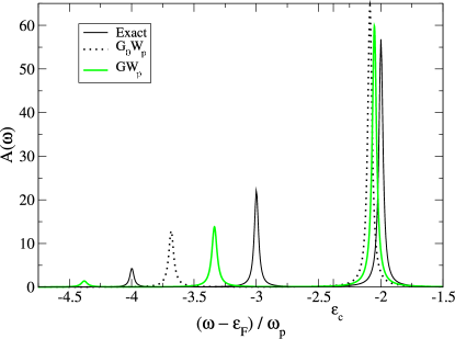
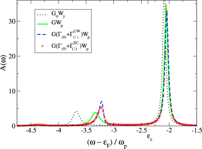
Figure 2: (Color online) Zero-temperature equilibrium spectral functions $A(\omega)$ for the for the high-density limit with $r_{S}=2$, corresponding to medium core electron-plasmon coupling $\gamma_{0}/\omega_{p}=0.62$. Top panel: Exact results and $GW$ calculations with and without self-consistency $\Sigma=GW_{p}$, $G_{0}W_{p}$. Bottom panel: Results for different levels of approximation for the self-energy $\Sigma=G_{0}W_{p}$, $GW_{p}$, $G(\Gamma_{(0)}+\Gamma_{(1)}^{GW})W_{p}$ and $G(\Gamma_{(0)}+\Gamma_{(1)}^{\rm SC})W_{p}$ (see Fig. 1) with fewer grid points ($N_{\omega}=1579$), giving an extra broadening.

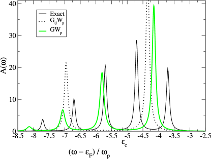
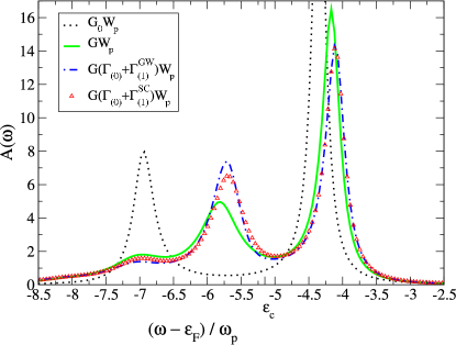
Figure 3: (Color online) Zero-temperature equilibrium spectral functions $A(\omega)$ for the low-density limit with $r_{S}=4$, corresponding to very strong core electron-plasmon coupling $\gamma_{0}/\omega_{p}=1.20$. Top panel: Exact results and $GW$ calculations for the different self-energies $\Sigma=G_{0}W_{p}$, $GW_{p}$. Bottom panel: Results for different levels of approximation for the self-energy $\Sigma=G_{0}W_{p}$, $GW_{p}$, $G(\Gamma_{(0)}+\Gamma_{(1)}^{GW})W_{p}$ and $G(\Gamma_{(0)}+\Gamma_{(1)}^{\rm SC})W_{p}$ (see Fig. 1) with fewer grid points ($N_{\omega}=1579$), giving an extra broadening, in comparison to the top panel.

The exact spectral function, calculated from the expression for the Green’s function given in Eq. (19), is shown as a solid black line in Figs. 2 and 3. A broadening equal to the broadening of our NEGF calculations has been applied. Fig. 2 shows the zero-temperature results for the high-density electron gas ($r_{S}=2$). The exact result provided by Eq. (19) (solid black line) gives a spectral function with a peak localized at the renormalized core level $\tilde{\varepsilon}_{c}=\varepsilon_{c}+D$, and plasmon side-band peaks at $\tilde{\varepsilon}_{c}-n\omega_{p}$ ($n\geq 1$) corresponding to plasmon emission. The peaks are hence separated by the plasmon energy $\omega_{p}$. In terms of amplitude, the main peak is that at $\tilde{\varepsilon}_{c}$ in the limit of weak to medium/strong electron-plasmon coupling, i.e. where $\gamma_{0}/\omega_{p}\leq 1$, and so for which $\gamma_{0}/\omega_{p}\leq 1$.

Fig. 3 shows the zero-temperature results for stronger coupling, $r_{S}=4$ and $\gamma_{0}/\omega_{p}>1$. Now the renormalized core level $\tilde{\varepsilon}_{C}$ has shifted to $\omega/\omega_{p}\sim 1.5$, while the spectral weight is shifted towards lower energies and the main peak is now the plasmon side-band peak at around $\omega/\omega_{p}$ Mahan (1990).

IV.4.2 Diagrammatic expansion results

The main differences between the exact result and the diagrammatic expansions of the self-energies and of the vertex functions (as represented in Fig. 1) are as follows:

First, let us discuss the results for the spectral functions in the high-density limit ($r_{S}=2$) for which the electron-plasmon coupling is medium $\gamma_{0}/\omega_{p}=0.62$.

The non-self-consistent $GW$ calculations (i.e. $\Sigma=G_{0}W_{p}$, Fig. 1(a), dotted black lines in Fig. 2) generate only two peaks, the renormalized core level with one plasmon side-band peak, as expected. However the positions of those two peaks are incorrect.

The self-consistent $GW$ calculations (i.e. $\Sigma=GW_{p}$, Fig. 1(b), solid green lines in Figs. 2 and 3) generate the correct series of plasmon side-band peaks. However the corresponding relaxation energy $D$ is too small and the energy position of the first plasmon side-band peak is too low. It should be noticed however that the energy separation between the plasmon side-band peaks is correctly reproduced, i.e. equal to $\omega_{p}$.

For the low-density limit ($r_{S}=4$) for which the electron-plasmon coupling is very strong $\gamma_{0}/\omega_{p}=1.20$, the $GW$ calculations poorly describe the exact spectral density. The self-consistent $GW$ calculations generate the correct series of peaks but with a completely wrong weight distribution. This is unsurprising since the $GW$ approach corresponds to a partial resummation of the diagrams, and does not include all other relevant diagrams necessary to deal with the very strong regime.

The lowest-order vertex corrections to the self-energy (Figs. 1(d) and 1(e), blue dashed lines and red triangles in Figs. 2 and 3) introduce modifications of the peak positions. They generate a slightly better relaxation energy $D$ and a shift of the side-band peaks towards the renormalized electron core level (Figs. 2 and 3, bottom panels). Vertex corrections globally improve the spectral information towards better overall agreement with the exact results. However, the lowest-order vertex correction expansion $\Gamma_{(0)}+\Gamma_{(1)}$ (see Appendix C) is still not sufficiently good to qualitatively reproduce the exact spectral functions in the limit of very strong electron-plasmon coupling.

The fully self-consistent calculations with $G\Gamma_{(1)}^{\rm SC}W_{p}$ seem to only marginally affect the lineshape of the plasmon side-band peaks in comparison to their non self-consistent counterpart.

Note that a fine analysis of the comparison between the exact results and the diagrammatic perturbation results with vertex correction is difficult to perform in Figs. 2 and 3, as the calculations were done for different numbers of $\omega$-grid points $N_{\omega}$. It was necessary to perform the calculations in that way because the vertex corrections scale as $N_{\omega}^{3}$ as shown in Ref. [Dash et al., 2010]. Therefore we have performed the corresponding calculations with a lower number of points $N_{\omega}=1579$ for the bottom panels of Figs. 2 and 3, instead of $N_{\omega}=16385$ points for the top panels, in order to have tractable computational costs. Our NEGF code works with a finite broadening related to the number of grid points to deal with sharply peaked and/or discontinuous functions, hence the different lineshape in the spectral functions in the top and bottom panels of Figs. 2 and 3 respectively. This numerical extra broadening affects only the width of the peaks and the global amplitude of the spectral functions, though all spectral functions are always normalized. There is no major problem with the spectral information contained in $A(\omega)$. We have discussed in detail the effects of this extra broadening in Ref. [Dash et al., 2010].

In addition, we want to add that our results confirm those obtained in earlier studies, see for example Refs. [Langreth, 1970; Minnhagen, 1975; Verdozzi et al., 1995; Shirley, 1996]. However our self-consistent scheme for calculating the second-order diagrams by starting with the $GW$-like Green’s function allows us to avoid the problem of negative spectral densities (at least within the range of parameters we have explored) that were obtained in Refs. [Minnhagen, 1974, 1975; Verdozzi et al., 1995].

IV.4.3 Finite temperatures

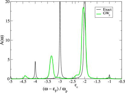
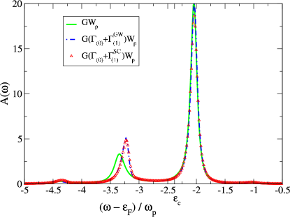
Figure 4: (Color online) Finite-temperature equilibrium spectral functions $A(\omega)$ for the high-density electron gas with $r_{S}=2$ and a finite temperature $kT=0.2$ corresponding to $\omega_{p}/kT=3.062$. Top panel: Exact results and calculations for different self-energies $\Sigma=GW_{p}$ and $GW^{(2){\rm SC}}_{p}$. Bottom panel: Results for different self-energies $\Sigma=GW_{p}$, $G(\Gamma_{(0)}+\Gamma_{(1)}^{GW})W_{p}$ and $G(\Gamma_{(0)}+\Gamma_{(1)}^{\rm SC})W_{p}$ (see Fig. 1) with fewer grid points ($N_{\omega}=1579$), giving an extra broadening.

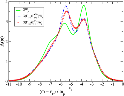
Figure 5: (Color online) Finite-temperature equilibrium spectral functions $A(\omega)$ for the low-density electron gas with $r_{S}=4$ and a finite temperature $kT=0.2$ (corresponding to $\omega_{p}/kT=1.083$) and with fewer grid points $N_{\omega}=1579$. Calculations for different self-energies $\Sigma=GW_{p}$, $GW^{(2){\rm SC}}_{p}$, $G(\Gamma_{(0)}+\Gamma_{(1)}^{GW})W_{p}$ and $G(\Gamma_{(0)}+\Gamma_{(1)}^{\rm SC})W_{p}$ (see Fig. 1) are shown.

For finite temperatures, the exact result provided by Eq. (19) can be generalized from a thermodynamical average over the boson statistics within a canonical ensembleMahan (1990); Ness (2006). In addition to the peaks at $\tilde{\varepsilon}_{c}-n\omega_{p}$ ($n\geq 0$), one also sees spectral information at $\tilde{\varepsilon}_{c}+n\omega_{p}$ ($n\geq 1$) which corresponds to absorption of the thermally populated plasmons, as shown in Figure 4.

The results for the spectral functions obtained from the diagrammatic expansion of the self-energy and of the vertex functions as shown in Fig. 1 are shown in Figs. 4 and 5. Qualitatively we obtain similar effects of the second-order diagrams on the spectral functions as in the case of zero temperature. Note that however, for finite temperatures, the dependence of the lineshape upon the extra broadening related to the number of $\omega$-grid points is much less important, since the thermal broadening is dominating. In Fig. 4 we see that, as for the zero-temperature case, the self-consistent $GW_{p}$ calculations generate the correct series of peaks with the plasmon emission sideband peaks again appearing at too low energies. However the new plasmon absorption peak just above the main peak is almost at the correct energy position.

We do not yet have an accurate explanation for the tiny shoulder-like feature around the Fermi level in the top panel of Fig. 4. However, this feature is related to plasmon absorption processes since at the chosen temperature the plasmon mode can be thermally populated. Nonetheless, it is clear that the feature disappears when performing the calculations with an extra broadening (i.e. introducing an effective finite lifetime for the plasmon mode).

When we consider the strong coupling case, shown in Fig. 5, we find that for all levels of approximation the lineshape is strongly broadened, washing out most of the features.

We can conclude that, within the limit of the S-model and for both the zero-temperature and finite-temperature cases, the various $GW$ approximations are much more accurate for the high-density regime. For the low-density electron gas both the $GW$ peak positions and lineshapes are poor in comparison to the exact results, although the separation between the plasmon sideband peaks is correctly reproduced.

IV.5 Spectral function of pure jellium and vertex corrections

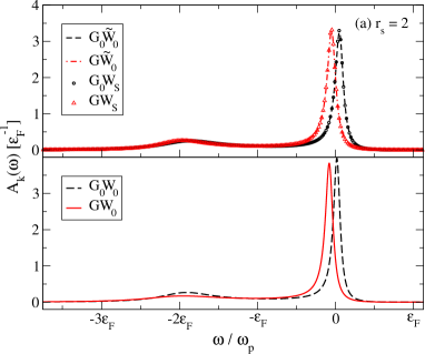
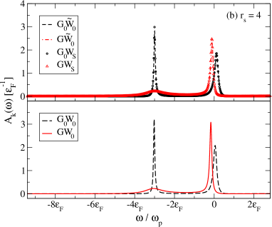
Figure 6: (Color online) Spectral function $A_{k}(\omega)$ at $k=0$ and for (a) $r_{\mathrm{S}}=2$ and (b) $r_{\mathrm{S}}=4$ for the pure jellium model. Each set of curves shows a one-shot calculation for $G_{0}$ (black data) and self-consistent iterations for $G$ (red data). The bottom panel of plots (a) and (b) show standard $G_{0}W_{0}$ and $GW_{0}$, the top panels show $G_{0}\tilde{W}_{0}$ and $G\tilde{W}_{0}$ with a local vertex correction in $\tilde{W}_{0}$ as described in Ref. [Del Sole et al., 1994]. $G_{0}W_{\mathrm{S}}$ and $GW_{\mathrm{S}}$ refer to a momentum-dependent vertex correction in $W_{\mathrm{S}}$ defined in Ref. [Shirley, 1996] to approximate the exact $W$ of jellium. The results including the different vertex corrections are indicated with a line (for $\tilde{W}_{0}$) and a symbol (for $W_{\mathrm{S}}$). All chemical potentials are aligned at the Fermi energy $\epsilon_{F}$ of the noninteracting gas. The positive (negative) deviation of the main quasiparticle peak from the origin indicates a narrowing (broadening) of the occupied bandwidth. None of these approximations provides more than one plasmon satellite in contrast to the expected exact result.

In this section, we compare different approximations for the vertex corrections for another model system: the pure jellium model (without a distinct core level). The spectral functions in this system are evaluated in the zero-temperature limit within conventional Green’s functions calculations Stankovski:unpub .

It is expected from the original work of Hedin et al. Hedin and Lundqvist (1969) and also of ShirleyShirley (1996) that the exact spectral function of pure jellium should show several plasmon resonances below the main quasiparticle peak. However, we do not observe any such peaks (see Fig. 6) when iterating the Green’s function to self-consistency within the $GW$ approximation, nor when we use model vertex corrections Del Sole et al. (1994); Shirley (1996). These vertex corrections were however supposed to provide an exact description of screened Coulomb interaction $W$ for the jellium model.

Any self-consistent iteration has the effect of broadening the occupied bandwidth (a feature which is known to be unphysical) as evidenced by the shift in the main quasiparticle peak at the bottom of the band seen in Fig. 6. The model vertex corrections tested do not remedy this behavior, nor do they lead to any multi-plasmon resonances. We consider two different models for the vertex corrections: Firstly, a strictly local vertex correction applied in the screening, annotated $\tilde{W}_{0}$ and modelled directly by the LDA exchange-correlation kernel as described by Del Sole et al. Del Sole et al. (1994). Secondly, the other vertex correction incorporates a momentum-dependent local field factor modelled on exact quantum Monte Carlo results for jellium, as described by Shirley Shirley (1996) (annotated $W_{\mathrm{S}}$).

In general, the difference between the two different types (static vs. $q$-dependent) of vertex corrections implemented is practically negligible in the spectral functions. This shows that the screened interaction can be very insensitive to the exact type of vertex correction used, in contrast to the self-energy. With a self-consistent calculation, we also observe the broadening of spectral peaks previously noted in Refs. [von Barth and Holm, 1996; Holm and von Barth, 1998].

This also indicates that the explicit evaluation of the second-order diagrammatic vertex correction, ${\Gamma}_{(1)}$, is imperative in order to capture the higher-order plasma sattelites in a metallic system, and in corresponding models with a coupling to a core state as shown in the previous section. This finding is fully consistent with the previous work of Shirley Shirley (1996) where the vertex function ${\Gamma}_{(1)}$ was approximately evaluated within the zero-temperature formalism.

V Conclusions

We have formally expressed the Hedin’s $GW$ equations on the Keldysh time-loop contour. This implies that within our formalism one can now deal with full non-equilibrium conditions for fully interacting electron systems. The equilibrium properties of the system are obtainable from our formalism as a special case of the more general non-equilibrium conditions.

We have considered in particular the lowest-order expansions of the electron self-energy $\Sigma$ and of the vertex function $\Gamma$, and compare our results with previous work. We have then used our formalism to study a simple model of an electron core level coupled to a plasmon mode for which exact results for the spectral function are available (i.e. the S-model). We have compared our lowest-order expansions of the electron self-energy and of the vertex function with the exact results, considering the second-order diagrams in terms of the plasmon propagator $W_{p}$.

We have shown that self-consistent $GW$-based approximations (with or without vertex corrections) provide a good approximation to the exact results in the limit of weak to medium electron-plasmon coupling (i.e. high electron-density limit) both at zero and finite temperatures. Non self-consistent $G_{0}W_{p}$ calculations do not reproduce the complete series of plasmon sattelites. However the $GW$ based approximations perform quite poorly in the strong-coupling limit (i.e. low electron-density limit). Vertex corrections generally re-adjust the peak positions (the relaxation energy responsible for the renormalization of the core level as well as the plasmon side-band peaks) towards the correct result.

Furthermore we have also analyzed the spectral functions obtained from conventional equilibrium $GW$ calculations for the pure jellium model and using different approximation for the vertex corrections in $W$. The corresponding results confirm that the explicit second order diagrams for the vertex corrections are needed to obtain the full series of plasmon side-band resonances.

In appendix D, we have also addressed an important issue about the Dyson-like equation for the time-ordered Green’s function in the energy represention. We have shown that there is a difference between Dyson equation for the Green’s function obtained at zero-temperature and at finite temperature, as already pointed out in Ref. [Hedin and Lundqvist, 1969]. We have shown that at finite temperature there are extra terms in the Dyson equation of the time-ordered Green’s function. These terms are obtained rigorously from the Keldysh time-loop formalism we derived at equilibrium, while they were introduced ad hoc by Hedin and Lundqvist Hedin and Lundqvist (1969) to recover an exact result.

Finally, we have studied in this paper models of interacting electron systems, but we believe that our theoretical approach is well-suited for applications towards more realistic physical systems, such as the one-dimensional plasmon modes recently observed in an atomic-scale metal wire deposited on a surface Nagao et al. (2006).

Appendix A Relationship between the different Green’s functions and self-energies

The relations between the different components of the Green’s functions and self-energies on the Keldysh time-loop contour are given as usual, with $X^{\eta_{1}\eta_{2}}(12)\equiv G^{\eta_{1}\eta_{2}}(12)$ or $\Sigma^{\eta_{1}\eta_{2}}(12)$.

$$\begin{split}X^{r}=X^{++}-X^{+-}&=X^{-+}-X^{--}\\ X^{a}=X^{++}-X^{-+}&=X^{+-}-X^{--}\\ X^{++}+X^{--}&=X^{+-}+X^{-+}\\ X^{-+}-X^{+-}&=X^{r}-X^{a}\end{split}$$ (20)

The usual lesser and greater projections are defined respectively as $X^{<}\equiv X^{+-}$ and $X^{>}\equiv X^{-+}$, and the usual time-ordered (anti-time-ordered) as $X^{t}=X^{++}$ ($X^{\tilde{t}}=X^{--}$).

Appendix B Rules for analytical continuation

For the following products $P_{(i)}(\tau,\tau^{\prime})$ on the time-loop contour $C_{K}$,

$$\begin{split}P_{(2)}&=\int_{C_{K}}AB\\ P_{(3)}&=\int_{C_{K}}ABC\\ P_{(n)}&=\int_{C_{K}}A_{1}A_{2}...A_{n},\\ \end{split}$$

we have the following rules for the different components $P_{(i)}^{x}(t,t^{\prime})$ on the real-time axis: $(x=r,a,>,<)$

$$\begin{split}P_{(2)}^{\gtrless}&=\int_{t}A^{r}B^{\gtrless}+A^{\gtrless}B^{a}\\ P_{(3)}^{<}&=\int_{t}A^{<}B^{a}C^{a}+A^{r}B^{<}C^{a}+A^{r}B^{r}C^{<}\\ P_{(n)}^{r}&=\int_{t}A_{1}^{r}A_{2}^{r}...A_{n}^{r}\ ,\hskip 14.22636ptP_{(n)}^{a}=\int_{t}A_{1}^{a}A_{2}^{a}...A_{n}^{a}.\end{split}$$

Appendix C Lowest order expansion of the vertex function $\Gamma(12;3)$

C.1 The $\Gamma_{(0)}$ level of approximation: no vertex corrections

In this section, we derive from our general results the more conventional $GW$ approach used in previous studies on the ground state properties of molecules, semi-conductors, or on the linear response or the full non-equilibrium transport properties of nanoscale systems driven by an applied external voltage Strange et al. (2011); Mera et al. (2010); Rostgaard et al. (2010); Spataru:2004 ; Spataru et al. (2009); Wang et al. (2008); Thygesen and Rubio (2007); Darancet et al. (2007).

With no vertex corrections, $\Gamma(12;3)$ is simply given by $\Gamma_{(0)}(12;3)=\delta(12)\delta(13)$. Hence the polarizability $\tilde{P}(12)$ and the electron self-energy $\Sigma(12)$ are

$$\begin{split}\tilde{P}(12)&=-{\rm i}G(12)\ G(21),\\ \Sigma(12)&={\rm i}G(12)\ W(21).\end{split}$$ (21)

The different components of the polarizability are then

$$\tilde{P}^{\lessgtr}(12)=-{\rm i}G^{\lessgtr}(12)\ G^{\gtrless}(21).$$ (22)

Using Eqs. (20), we find that the retarded polarizability is given by

$$\begin{split}\tilde{P}^{r}(12)&=-{\rm i}[G(12)\ G(21)]^{r}\\ &=-{\rm i}G^{r}(12)\ G^{<}(21)-{\rm i}G^{<}(12)\ G^{a}(21),\end{split}$$ (23)

and the electron self-energy by

$$\begin{split}\Sigma^{<}(12)&={\rm i}G^{<}(12)\ W^{>}(21),\\ \Sigma^{r}(12)&={\rm i}[G(12)\ W(21)]^{r}\\ &={\rm i}G^{r}(12)\ W^{<}(21)+{\rm i}G^{<}(12)\ W^{a}(21).\end{split}$$ (24)

Using the symmetry relations for $W$ and Eqs. (20), we can easily recast the above equations in the following form

$$\begin{split}\Sigma^{<}(12)&={\rm i}G^{<}(12)\ W^{<}(12)\\ \Sigma^{r}(12)&={\rm i}G^{r}(12)\ W^{>}(12)+{\rm i}G^{<}(12)\ W^{r}(12).\end{split}$$ (25)

These expressions for $\Sigma$ and $\tilde{P}$ are just the equivalent of Eqs. (3-8) in Ref. [Thygesen and Rubio, 2007] and are similar to the corresponding expressions in Refs. [Stan et al., 2009a, b; Rostgaard et al., 2010; Spataru:2004, ].

C.2 The $\Gamma_{(1)}$ level of approximation

With the series expansion $\Gamma(12;3)=\sum_{n}\Gamma_{(n)}(12;3)$, in which the index $n$ represents the number of times the screened Coulomb interaction $W$ appears explicitly in the series, we take for $\Gamma_{(1)}(12;3)$

$$\Gamma_{(1)}(12;3)=\int{\rm d}(4567)\ \frac{\delta\Sigma(12)}{\delta G(45)}G(46)G(75)\Gamma(67;3),$$ (26)

where$\Gamma(67;3)=\Gamma_{(0)}(67;3)=\delta(67)\delta(63)$ and $\Sigma={\rm i}GW$. Hence $\Gamma_{(1)}(12;3)={\rm i}W(21)\ G(13)\ G(32)$.

In the following, we derive the part of the electron self-energy and the part of the polarizability arising from $\Gamma_{(1)}$ only. In principle, the full $\Sigma$ and $\tilde{P}$ should be calculated by using $\Gamma=\Gamma_{(0)}+\Gamma_{(1)}$. We find for the electron self-energy (defined on the contour $C_{K}$):

$$\begin{split}\Sigma(12)&={\rm i}\int{\rm d}(34)\ G(13)\ \Gamma_{(1)}(32;4)\ W(4,1)\\ &={\rm i}\times{\rm i}\int{\rm d}(34)\ G(13)\ W(23)\ G(34)\ G(42)\ W(41).\end{split}$$ (27)

The different components $\Sigma^{\eta_{1}\eta_{2}}$ of the self-energy on the time-loop contour (with $\eta_{1,2}=\pm$) are then given by

$$\begin{split}\Sigma^{\eta_{1}\eta_{1}}(12)=-\sum_{\eta_{3}\eta_{4}}\ &\eta_{3}\eta_{4}\int{\rm d}(34)\ G^{\eta_{1}\eta_{3}}(13)\ W^{\eta_{2}\eta_{3}}(23)\\ &G^{\eta_{3}\eta_{4}}(34)\ G^{\eta_{4}\eta_{2}}(42)\ W^{\eta_{4}\eta_{1}}(41).\end{split}$$ (28)

This self-energy corresponds to the so-called double-exchange diagram. Note that we have studied the effects of such a diagram in the different context of a propagating electron coupled to a local vibration mode, in which the bosonic propagator $W$ is replaced by a phonon propagator $D$Dash et al. (2010).

At the $\Gamma_{(1)}$ level of approximation, we find that the polarizability is given by

$$\begin{split}\tilde{P}(12)&=-{\rm i}\int{\rm d}(34)\ G(13)\ G(41)\ \Gamma_{(1)}(34;2)\\ &=\int{\rm d}(34)\ G(13)\ G(41)\ W(43)\ G(24)\ G(32),\end{split}$$ (29)

with components on $C_{K}$ given by

$$\begin{split}\tilde{P}^{\eta_{1}\eta_{2}}(12)=\sum_{\eta_{3}\eta_{4}}\ &\eta_{3}\eta_{4}\int{\rm d}(34)G^{\eta_{1}\eta_{3}}(13)\ G^{\eta_{4}\eta_{1}}(41)\\ &W^{\eta_{4}\eta_{3}}(43)\ G^{\eta_{2}\eta_{4}}(24)\ G^{\eta_{3}\eta_{2}}(32).\end{split}$$ (30)

Here again, and as well as for the self-energy, the retarded (advanced) part $\tilde{P}^{r}(12)$ is obtained from $\tilde{P}^{r}=\tilde{P}^{++}-\tilde{P}^{+-}$. One can then express $\tilde{P}^{r}$ and $\tilde{P}^{+-}$ in a more compact form involving only terms like $X^{r,a,\lessgtr}$ (with $X\equiv G,W$).

Appendix D Time-ordered Green’s functions at equilibrium

In this section we discuss in detail the relation between time-ordered Green’s function (in energy representation) for two temperature limits. Differences are expected to arise as shown in Chapter IV.17. of Ref. [Hedin and Lundqvist, 1969]. We use the conventional equilibrium many-body perturbation theory (MBPT) to determine the time-ordered Green’s function $G^{t}$, and the generalization of the Green’s function onto the Keldysh time-loop contour at equilibrium to determine the counterpart of the time-ordered Green’s function $G^{++}$.

From MBPT, the time-ordered Green’s function satisfies the Dyson-like equation $G^{t}=g^{t}+g^{t}\Sigma^{t}G^{t}$ and the corresponding time-ordered Green’s function obtained from the Keldysh time-loop expansion satisfies the corresponding Dyson-like equation $G^{++}=g^{++}+(g\Sigma G)^{++}$. In principle, from the conventional definition we have $g^{t}=g^{++}$ and and should have $G^{t}=G^{++}$.

It is easy to show that from the rules of analytical continuation $G^{++}=g^{++}+(g\Sigma G)^{++}$ is expanded as follows

$$\begin{split}G^{++}&=g^{++}+g^{++}\Sigma^{++}G^{++}\\ &-g^{++}\Sigma^{<}G^{>}+g^{<}\Sigma^{>}G^{++}+g^{<}\Sigma^{--}G^{++},\end{split}$$ (31)

and after further manipulation (using the notation $(g/G)^{t}=(g/G)^{++}$),

$$G^{t}=g^{t}+\left(g^{t}\Sigma^{t}-g^{<}\Sigma^{>}\right)G^{t}-(g\Sigma)^{<}G^{>}.$$ (32)

So, strictly speaking, the non-equilibrium formalism introduces two extra terms $g^{<}\Sigma^{>}G^{t}$ and $(g\Sigma)^{<}G^{>}$ in the Dyson equation for $G^{t}$.

We now analyze these two terms in more detail. First of all, we recall that at equilibrium or in a steady state, the Green’s functions and self-energies depend only on the time difference of their argument and can be Fourier transformed with a single energy argument. We then have the following expression

$$\begin{split}G^{t}(\omega)=g^{t}(\omega)&+\left(g^{t}(\omega)\Sigma^{t}(\omega)-g^{<}(\omega)\Sigma^{>}(\omega)\right)G^{t}(\omega)\\ &-(g\Sigma)^{<}(\omega)G^{>}(\omega).\end{split}$$ (33)

Furthermore, at equilibrium or in a steady state, the lesser and greater components of either a Green’s function or a self-energy ($X^{\lessgtr}$) can be expressed in terms of the corresponding advanced and retarded quantity and a distribution function Ness et al. (2010); Kita (2010); Meden et al. (1995); Lipavský et al. (1986), i.e.

$$X^{\lessgtr}(\omega)=-f^{\lessgtr}(\omega)(X^{r}(\omega)-X^{a}(\omega)).$$ (34)

At equilibrium $f^{\lessgtr}(\omega)=f_{0}^{\lessgtr}(\omega)$ and for a system of fermoins, $f_{0}^{<}$ is given by the Fermi-Dirac distribution function $f^{\rm eq}(\omega)=1/(1+\exp\beta(\omega-\mu^{\rm eq}))$ and $f_{0}^{>}=f^{\rm eq}-1$ (with $\beta=1/kT$).

At zero temperature, the Fermi-Dirac distribution takes only two different values, $f^{\rm eq}=1$ or $0$. Hence we have the property $(f^{\rm eq})^{2}=f^{\rm eq}$, which implies that $f_{0}^{<}(\omega)f_{0}^{>}(\omega)=f^{\rm eq}(f^{\rm eq}-1)=0$. Consequently any products of the kind $X^{<}(\omega)Y^{>}(\omega)$ or $X^{>}(\omega)Y^{<}(\omega)$ vanish. Therefore we recover from the Keldysh time-loop formalism Eq. (33) at zero temperature, the conventional Dyson equation $G^{t}=g^{t}+g^{t}\ \Sigma^{t}\ G^{t}$ as expected.

At finite temperature $f_{0}^{<}(\omega)f_{0}^{>}(\omega)=f^{\rm eq}(f^{\rm eq}-1)=kT\partial_{\omega}f^{\rm eq}\neq 0$, and the product $f_{0}^{<}f_{0}^{>}$ gives a sharply peaked function at the Fermi level $\mu^{\rm eq}=\varepsilon_{F}$ with a width of approximately $kT$.

We now check the individual contribution of each term $g^{<}\Sigma^{>}$ and $(g\Sigma)^{<}G^{>}$, first for a specific case (i.e. the quasi-particle approximation) and then for the general case.

In a quasi-particle scheme, i.e. when a single index $k$ is good enough to represent the quantum states (with energy $\varepsilon_{k}$), the Green’s functions and the self-energies in the absence and in the presence of interaction are diagonal in this representation. We have

$$\begin{split}&g^{<}_{k}(\omega)\Sigma^{>}_{k}(\omega)\\ &=-f_{0,k}^{<}(g^{r}_{k}-g^{a}_{k})(\omega)\times-f_{0,k}^{>}(\Sigma^{r}_{k}-\Sigma^{a})(\omega)\\ &=4\pi f_{0,k}^{<}f_{0,k}^{>}\delta(\omega-\varepsilon_{k})\ \Im m\Sigma^{r}_{k}(\omega).\end{split}$$ (35)

For purely fermionic systems at equilibrium, one usually has $\Im m\Sigma^{r}_{k}(\mu^{\rm eq})=0$ Benedict:2002 , and therefore $g^{<}_{k}(\mu^{\rm eq})\Sigma^{>}_{k}(\mu^{\rm eq})=0$. When $\Im m\Sigma^{r}_{k}$ also vanishes in the energy window around the Fermi level, defined by $f_{0}^{<}f_{0}^{>}\neq 0$, then the product $g^{<}_{k}(\omega)\Sigma^{>}_{k}(\omega)$ also vanishes. When there are no eigenvalues $\varepsilon_{k}$ (of the non-interacting system) within this energy window, then once more we have $g^{<}_{k}(\omega)\Sigma^{>}_{k}(\omega)\sim 0$.

Otherwise $g^{<}_{k}(\omega)\Sigma^{>}_{k}(\omega)=\tilde{Z}_{k}\delta(\omega-\varepsilon_{k})$ with $\tilde{Z}_{k}=4\pi\left(f_{0}^{<}f_{0}^{>}\Im m\Sigma^{r}_{k}(\omega)\right)_{\omega=\varepsilon_{k}}$.

For the second correction term, we have

$$\begin{split}&(g\Sigma)_{k}(\omega)^{<}G^{>}_{k}(\omega)\\ &=-f_{0,k}^{<}((g\Sigma)^{r}_{k}-(g\Sigma)^{a}_{k})(\omega)\times-f_{0,k}^{>}(G^{r}_{k}-G^{a}_{k})(\omega)\\ &=f_{0,k}^{<}(g^{r}_{k}\Sigma^{r}_{k}-g^{a}_{k}\Sigma^{a}_{k})(\omega)\ f_{0,k}^{>}(G^{r}_{k}-G^{a}_{k})(\omega).\end{split}$$ (36)

For the quasi-particle scheme, $\Im m\Sigma^{r/a}_{k}\sim\pm{\rm i}\eta$ around the Fermi level $\mu^{\rm eq}\pm kT$, and we find that

$$(g_{k}\Sigma_{k})^{<}G^{>}_{k}=-4\pi f_{0}^{<}f_{0}^{>}Z_{k}\Re e\Sigma^{r}_{k}(\varepsilon_{k})\ \delta(\omega-\varepsilon_{k})\delta(\omega-\tilde{\varepsilon}_{k})$$ (37)

with $Z_{k}^{-1}=1-(\partial\Re e\Sigma^{r}_{k}/\partial\omega)_{\omega=\tilde{\varepsilon}_{k}}$ being the effective mass renormalisation parameter and $\tilde{\varepsilon}_{k}=\varepsilon_{k}+\Re e\Sigma^{r}_{k}$ being the renormalized eigenvalue. Hence the product $(g_{k}\Sigma_{k})^{<}G^{>}_{k}$ vanishes because in general one has $\tilde{\varepsilon}_{k}\neq\varepsilon_{k}$. In the opposite case when $\tilde{\varepsilon}_{k}=\varepsilon_{k}$ for some quantum states, the product $(g_{k}\Sigma_{k})^{<}G^{>}_{k}$ also vanishes because then $\Re e\Sigma^{r}_{k}=0$.

Therefore our analysis show that, in the quasi-particle scheme at finite temperature, Eq. (33) reduces to the conventional Dyson equation $G^{t}_{k}=g^{t}_{k}+g^{t}_{k}\ \Sigma^{t}_{k}\ G^{t}_{k}$ as expected.

Now we need to check what is happening to the two contributions $g^{<}\Sigma^{>}$ and $(g\Sigma)^{<}G^{>}$ beyond the quasi-particle approximation. For that we can proceed further: going back to the full time-dependence of Eq. (32) and factorizing the non-interacting time-ordered Green’s function $g^{t}$:

$$G^{t}=g^{t}\left(1+\left(\Sigma^{t}-(g^{t})^{-1}g^{<}\Sigma^{>}\right)G^{t}-(g^{t})^{-1}(g\Sigma)^{<}G^{>}\right),$$ (38)

with $(g\Sigma)^{<}=g^{<}\Sigma^{a}+g^{r}\Sigma^{<}$.

By using the equation of motion of the non-interacting time-ordered Green’s function $g^{t}$:

$$\left({\rm i}\frac{\partial}{\partial t_{1}}-h_{0}(1)\right)g^{t}(12)=\delta(12),$$ (39)

it is straightforward to find that

$$(g^{t})^{-1}(13)=\left({\rm i}\frac{\partial}{\partial t_{1}}-h_{0}(1)\right)\delta(13).$$ (40)

and consequently

$$\begin{split}(g^{t})^{-1}g^{<}(14)&\equiv\int{\rm d}3\ (g^{t})^{-1}(13)g^{<}(34)\\ &=\left({\rm i}\frac{\partial}{\partial t_{1}}-h_{0}(1)\right)g^{<}(14)=0,\end{split}$$ (41)

the last equality comes from the definition of $g^{<}(14)$. Similarly one can find that $(g^{t})^{-1}g^{r}\equiv\int{\rm d}3\ (g^{t})^{-1}(13)g^{r}(34)=\delta(14)$.

Hence Eq. (38) is transformed into

$$G^{t}=g^{t}+g^{t}\Sigma^{t}G^{t}-\Sigma^{<}G^{>},$$ (42)

where the last term $\Sigma^{<}G^{>}$ satisfies the detailed balance equation at equilibrium Danielewicz (1984a): $\Sigma^{<}G^{>}=\Sigma^{>}G^{<}$.

Eq. (42) is the most general expression for $G^{t}$ and is the most important result of this section. It is interesting to note that Eq. (42) is the equivalent of Eq. (17.9) derived in Ref. [Hedin and Lundqvist, 1969]. However in our approach, the extra term $\Sigma^{<}G^{>}$ is obtained rigorously from the use of the general Keldysh time-loop contour formalism. While in Ref. [Hedin and Lundqvist, 1969], Hedin and Lundqvist introduced this correction term ad hoc in the Dyson equation for the finite temperature time-ordered Green’s function in order to recover the proper limit of the independent particle case.

Once more one can show that, after Fourier transforming, the product $\Sigma^{<}G^{>}$ vanishes at equilibrium and at zero temperature because of Eq. (33) and $f_{0}^{<}f_{0}^{>}=0$. Within the quasi-particle scheme at finite temperature, we have $\Sigma^{<}_{k}(\omega)G^{>}_{k}(\omega)=-4f_{0,k}^{<}f_{0,k}^{>}\ \Im m\Sigma^{r}_{k}(\omega)\ \Im mG^{r}_{k}(\omega)$. Thus, one needs to check the contributions of the spectral information in $\Im m\Sigma^{r}_{k}(\omega)$ and in $\Im mG^{r}_{k}(\omega)$ (in the energy window defined by $f_{0,k}^{<}f_{0,k}^{>}$ around the Fermi level) to see if the product $\Sigma^{<}_{k}G^{>}_{k}$ vanishes (as shown above).

We conclude this appendix by saying that there is indeed a difference between the Dyson equations for the time-ordered Green’s functions at zero and finite temperature Hedin and Lundqvist (1969); Fetter and Walecka (1971)^,. This result by no means contradicts the fact that the Green’s functions on the Keldysh contour, the time-ordered Green’s function at zero temperature and the Matsubara temperature Green’s function of imaginary argument all obey the same formal Dyson equation. Our derivations provide a rigorous mathematical result for the finite temperature time-ordered Green’s function (in the energy representation) which satisfies a Dyson equation with an extra term as introduced in an ad-hoc way in Chap IV.17. of Ref. [Hedin and Lundqvist, 1969].

In our calculations, the correction term $\Sigma^{<}G^{>}$ is automatically taken into account since we work with the Keldysh time-loop formalism. We have checked numerically that the $\Sigma^{<}G^{>}$ indeed vanishes at zero temperature. For finite temperatures we have found that $\Sigma^{<}G^{>}\sim 0$ in the energy window defined by $f_{0}^{<}f_{0}^{>}\neq 0$ since most of the spectral weight is far below the Fermi level (see Figures 2 to 5). However, in the limit of very high temperatures (i.e. $\omega_{p}/kT\ll 1$), the energy window defined by $f_{0}^{<}f_{0}^{>}\neq 0$ is wide and the product $\Sigma^{<}G^{>}$ does not vanish; though the corrections are two orders of magnitude smaller than the amplitude of the Green’s function $G^{t}$ itself.

It would be interesting to find real cases of interacting electron systems (probably of low dimensionality) for which the correction term $\Sigma^{<}G^{>}$ is not negligible. At finite but low temperatures, systems with a strong spectral density around the Fermi level (i.e. presenting the Kondo effect) at low temperature should be a good example. The high temperature limit for metallic systems represents another interesting case as shown, for example, in Ref. [Benedict:2002, ].

References

- Abrikosov et al. (1963) A. A. Abrikosov, L. P. Gorkov, and I. E. Dzyaloshinski, Methods of Quantum Field Theory in Statistical Physics (Dover, New York, 1963).
- Hedin (1965) L. Hedin, Physical Review 139, A796 (1965).
- Hedin and Lundqvist (1969) L. Hedin and S. Lundqvist, Effects of Electron-Electron and Electron-Phonon Interactions on the One-Electron States of Solids, vol. 23 of Solid State Physics (Academic Press, New York, 1969).
- Godby et al. (1988) R. W. Godby, M. Schlüter, and L. J. Sham, Phys. Rev. B 37, 10159 (1988).
- Del Sole et al. (1994) R. Del Sole, L. Reining, and R. W. Godby, Phys. Rev. B 49, 8024 (1994).
- Aryasetiawan and Gunnarsson (1998) F. Aryasetiawan and O. Gunnarsson, Reports on Progress in Physics 61, 237 (1998).
- Rieger et al. (1999) M. M. Rieger, L. Steinbeck, I. D. White, H. N. Rojas, and R. W. Godby, Comp. Phys. Comm. 117, 211 (1999).
- Onida et al. (2002) G. Onida, L. Reining, and A. Rubio, Rev. Mod. Phys. 74, 601 (2002).
- Rohlfing et al. (1995) M. Rohlfing, P. Krüger, and J. Pollmann, Phys. Rev. B 52, 1905 (1995).
- Rohlfing and Louie (2000) M. Rohlfing and S. G. Louie, Phys. Rev. B 62, 4927 (2000).
- (11) L. X. Benedict, C. D. Spataru, and S. G. Louie, Phys. Rev. B 66, 085116 (2002).
- Blase et al. (2011) X. Blase, C. Attaccalite, and V. Olevano, Physical Review B 83, 115103 (2011).
- Faber et al. (2011) C. Faber, C. Attaccalite, V. Olevano, E. Runge, and X. Blase, Physical Review B 83, 115123 (2011).
- Keldysh (1965) L. Keldysh, Sov. Phys. JETP 20, 1018 (1965).
- Wagner (1991) M. Wagner, Physical Review B 44, 6104 (1991).
- Danielewicz (1984a) P. Danielewicz, Annals of Physics 152, 239 (1984a).
- van Leeuwen et al. (2006) R. van Leeuwen, N. E. Dahlen, G. Stefanucci, C.-O. Almbladh, and U. von Barth, Lecture Notes in Physics 706, 33 (2006).
- Haug and Jauho (1996) H. Haug and A. P. Jauho, Quantum Kinetics in Transport and Optics of Semi-conductors (Springer-Verlag, Berlin, 1996).
- Myöhänen et al. (2009) P. Myöhänen, A. Stan, G. Stefanucci, and R. van Leeuwen, Physical Review B 80, 115107 (2009).
- Myöhänen et al. (2008) P. Myöhänen, A. Stan, G. Stefanucci, and R. van Leeuwen, EuroPhysics Letters 84, 67001 (2008).
- Rammer (2007) J. Rammer, Quantum Field Theory of Non-Equilibrium States (Cambridge University Press, Cambridge, 2007).
- Stefanucci and Almbladh (2004) G. Stefanucci and C.-O. Almbladh, Physical Review B 69, 195318 (2004).
- Rammer (1991) J. Rammer, Review of Modern Physics 63, 781 (1991).
- Rammer and Smith (1986) J. Rammer and H. Smith, Review of Modern Physics 58, 323 (1986).
- Danielewicz (1984b) P. Danielewicz, Annals of Physics 152, 305 (1984b).
- Schwinger (1961) J. Schwinger, J. Math. Phys. 2, 407 (1961).
- chao Chou et al. (1985) K. chao Chou, Z. bin Su, B. lin Hao, and L. Yu, Physics Reports 118, 1 (1985).
- (28) C. D. Spataru, L. X. Benedict, and S. G. Louie, Phys. Rev. B 69, 205204 (2004).
- Stan et al. (2006) A. Stan, N. E. Dahlen, and R. van Leeuwen, Europhysics Letters 76, 298 (2006).
- Dahlen and van Leeuwen (2007) N. E. Dahlen and R. van Leeuwen, Physical Review Letters 98, 153004 (2007).
- Stan et al. (2009a) A. Stan, N. E. Dahlen, and R. van Leeuwen, J. Chem. Phys. 130, 114105 (2009a).
- Stan et al. (2009b) A. Stan, N. E. Dahlen, and R. van Leeuwen, J. Chem. Phys. 130, 224101 (2009b).
- Thygesen and Rubio (2007) K. S. Thygesen and A. Rubio, Journal of Chemical Physics 126, 091101 (2007).
- Rostgaard et al. (2010) C. Rostgaard, K. W. Jacobsen, and K. S. Thygesen, Physical Review B 81, 085103 (2010).
- (35) M. Puig von Friesen and C. Verdozzi and C.-O. Almbladh, Physical Review Letters, 103, 176404 (2009).
- (36) M. Puig von Friesen and C. Verdozzi and C.-O. Almbladh, Physical Review B, 82, 155108 (2010).
- Harbola and Mukamel (2006) U. Harbola and S. Mukamel, Journal of Chemical Physics 124, 044106 (2006).
- Langreth (1970) D. C. Langreth, Phys. Rev. B 1, 471 (1970).
- Minnhagen (1975) P. Minnhagen, Journal of Physics C: Solid State Physics 8, 1535 (1975).
- Aulbur et al. (2000) W. G. Aulbur, C. Jönsson, and J. W. Wilkins, Solid State Physics 54, 1 (2000).
- Rinke et al. (2008) P. Rinke, A. Qteish, J. Neugebauer, and M. Scheffler, phys. stat. sol. (b) 4245, 929 (2008).
- van Schilfgaarde et al. (2006) M. van Schilfgaarde, T. Kotani, and S. Faleev, Physical Review Letters 96, 226402 (2006).
- deGroot et al. (1995) H. J. deGroot, P. A. Bobbert, and W. van Haeringen, Physical Review B 52, 11000 (1995).
- von Barth and Holm (1996) U. von Barth and B. Holm, Physical Review B 54, 8411 (1996).
- Shirley (1996) E. L. Shirley, Phys. Rev. B 54, 7758 (1996).
- Romaniello et al. (2009) P. Romaniello, S. Guyot, and L. Reining, Journal of Chemical Physics 131, 154111 (2009).
- Holm and von Barth (1998) B. Holm and U. von Barth, Physical Review B 57, 2108 (1998).
- Holm (1999) B. Holm, Physical Review Letters 83, 788 (1999).
- García-González and Godby (2001) P. García-González and R. Godby, Physical Review B 63, 075112 (2001).
- Baym and Kadanoff (1961) G. Baym and L. P. Kadanoff, Physical Review 124, 287 (1961).
- Kaasbjerg and Thygesen (2010) K. Kaasbjerg and K. S. Thygesen, Physical Review B 81, 085102 (2010).
- Kutepov et al. (2009) A. Kutepov, S. Y. Savrasov, and G. Kotliar, Physical Review B 80, 041103(R) (2009).
- Faleev et al. (2004) S. Faleev, M. van Schilfgaarde, and T. Kotani, Physical Review Letters 93, 126406 (2004).
- Shishkin et al. (2007) M. Shishkin, M. Marsman, and G. Kresse, Physical Review Letters 99, 246403 (2007).
- Jiang et al. (2009) H. Jiang, R. Gomez-Abal, P. Rinke, and M. Scheffler, Physical Review Letters 102, 126403 (2009).
- Chantis et al. (2007) A. N. Chantis, M. van Schilfgaarde, and T. Kotani, Physical Review B 76, 165126 (2007).
- Giantomassi et al. (2011) M. Giantomassi, M. Stankovski, R. Shaltaf, M. Grüning, F. Bruneval, P. Rinke, and G.-M. Rignanese, phys. stat. sol. (b) 248, 275 (2011).
- Ness (2006) H. Ness, Journal of Physics: Condensed Matter 18, 6307 (2006).
- Dash et al. (2010) L. K. Dash, H. Ness, and R. W. Godby, Journal of Chemical Physics 132, 104113 (2010).
- Dash et al. (2011) L. K. Dash, H. Ness, and R. W. Godby, Phys. Rev. B 84, 085433 (2011).
- Mahan (1990) G. D. Mahan, Many-Particle Physics (Plenum Press, New York, 1990).
- Verdozzi et al. (1995) C. Verdozzi, R. W. Godby, and S. Holloway, Phys. Rev. Lett. 74, 2327 (1995).
- Minnhagen (1974) P. Minnhagen, Journal of Physics C: Solid State Physics 7, 3013 (1974).
- (64) M. Stankovski et al., unpublished.
- Ness et al. (2010) H. Ness, L. Dash, and R. W. Godby, Physical Review B 82, 085426 (2010).
- Kita (2010) T. Kita, Progress of Theoretical Physics 123, 581 (2010).
- Meden et al. (1995) V. Meden, C. Wöhler, J. Fricke, and K. Schönhammer, Physical Review B 52, 5624 (1995).
- Lipavský et al. (1986) P. Lipavský, V. Špička, and B. Velický, Physical Review B 34, 6933 (1986).
- Fetter and Walecka (1971) A. L. Fetter and J. D. Walecka, Quantum Theory of Many-Particle Systems (McGraw-Hill, New York, 1971).
- Nagao et al. (2006) T. Nagao, S. Yaginuma, T. Inaoka, and T. Sakurai, Physical Review Letters 97, 116802 (2006).
- Strange et al. (2011) M. Strange, C. Rostgaard, H. Häkkinen, and K. S. Thygesen, Physical Review B 83, 115108 (2011).
- Mera et al. (2010) H. Mera, K. Kaasbjerg, Y. M. Niquet, and G. Stefanucci, Phys. Rev. B 81, 035110 (2010).
- Spataru et al. (2009) C. D. Spataru, M. S. Hybertsen, S. G. Louie, and A. J. Millis, Physical Review B 79, 155110 (2009).
- Wang et al. (2008) X. Wang, C. D. Spataru, M. S. Hybertsen, and A. J. Millis, Physical Review B 77, 045119 (2008).
- Darancet et al. (2007) P. Darancet, A. Ferretti, D. Mayou, and V. Olevano, Phys. Rev. B 75, 075102 (2007).