The $J_{1}-J_{2}$ Heisenberg model at and close to its $z=4$ quantum critical point

Abstract

We study the frustrated $J_{1}-J_{2}$ Heisenberg model with ferromagnetic nearest neighbor coupling $J_{1}<0$ and antiferromagnetic next-nearest neighbor coupling $J_{2}>0$ at and close to the $z=4$ quantum critical point (QCP) at $J_{1}/J_{2}=-4$. The $J_{1}-J_{2}$ model plays an important role for recently synthesized chain cuprates as well as in supersymmetric Yang Mills theories. We study the thermodynamic properties using field theory, a modified spin-wave theory as well as numerical density-matrix renormalization group calculations. Furthermore, we compare with results for the classical model obtained by analytical methods and Monte-Carlo simulations. As one of our main results we present numerical evidence that the susceptibility at the QCP seems to diverge with temperature $T$ as $\chi\sim T^{-1.2}$ in the quantum case in contrast to the classical model where $\chi\sim T^{-4/3}$.

I Introduction

The frustrated one-dimensional (1D) $s=1/2$ Heisenberg model

$$H=J_{1}\sum_{j}\boldsymbol{S}_{j}\boldsymbol{S}_{j+1}+J_{2}\sum_{j}\boldsymbol{S}_{j}\boldsymbol{S}_{j+2}$$ (1)

with nearest neighbor coupling $J_{1}$ and next-nearest neighbor coupling $J_{2}$ is the minimal model to describe magnetism in a number of cuprate chain compounds. It can be viewed as a ladder with coupling $J_{2}$ along the legs and a zigzag rung coupling $J_{1}$ as shown in Fig. 1(a). Recently, there has been renewed interest in this model with ferromagnetic coupling $J_{1}<0$ and antiferromagnetic coupling $J_{2}>0$ propelled by the discovery of multiferroic behavior in edge sharing spin chains.et al. (2007); Masuda et al. (2004); Park et al. (2007); Seki et al. (2008); Drechsler et al. (2007); Katsura et al. (2005); Mostovoy (2006) The phase diagram of this model as a function of $\tilde{\alpha}=J_{1}/J_{2}$ has been studied by a combination of field theoretical and numerical methods.Tonegawa and Harada (1987); Chitra et al. (1995); White and Affleck (1996); Itoi and Qin (2001); Bursill et al. (1995); Nersesyan et al. (1998) It is shown schematically in Fig. 1(b). At $\tilde{\alpha}=0$ the system consists of two decoupled, critical antiferromagnetic Heisenberg chains. By bosonization it has been found that a small coupling, $|J_{1}|\ll 1$, leads to an exponentially small gap $\Delta\propto\exp(-\mbox{const}\,|\tilde{\alpha}|)$.White and Affleck (1996); Itoi and Qin (2001); Nersesyan et al. (1998) On the antiferromagnetic side, $\tilde{\alpha}>0$, the gapped phase exists up to a critical point (QCP2 in Fig. 1(b)) at $\tilde{\alpha}\approx 4.15$Okamoto and Nomura (1992) where the system enters a critical gapless phase. At the so-called Majumdar-Ghosh (MG) point,Majumdar and Ghosh (1969) $\tilde{\alpha}=2$, the ground state is known exactly and consists of decoupled dimers.

Figure 1: (a) The $J_{1}-J_{2}$ chain viewed as a ladder with zigzag coupling. (b) Phase diagram of the $J_{1}-J_{2}$ chain as a function of $J_{1}/J_{2}$ with $J_{2}>0$.

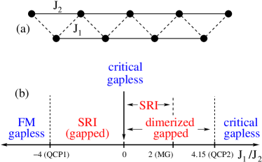
Dimerization is indeed present for the whole gapped phase $0<\tilde{\alpha}\lesssim 4.15$ while short-ranged incommensurate (SRI) spin correlations have only been found for $0<\tilde{\alpha}<2$.Chitra et al. (1995); White and Affleck (1996) On the ferromagnetic side, $\tilde{\alpha}<0$, a phase with incommensurate spin-spin correlations is followed by a ferromagnetic phase. The transition occurs at $\tilde{\alpha}=-4$ (QCP1 in Fig. 1(b)), both in the quantum as well as in the classical model.Bader and Schilling (1979); Härtel et al. (2008) Whereas the incommensurate (“spiral”) correlations are long-ranged in the classical model, these correlations are predicted to be short-ranged in the quantum model.Nersesyan et al. (1998) However, the gap is expected to be exponentially small and no numerical evidence for this gap has been found yet.Itoi and Qin (2001); Sirker (2010); Sudan et al. (2009) At the critical point QCP1, the ferromagnetic state and states of resonance valence bond (RVB) character are degenerate.HamadaKane In fact, all degenerate ground states at this point can be explicitly constructed.SuzukiTakano1 ; SuzukiTakano2 It turns out that there exists a unique ground state for a fixed total spin $S_{\rm tot}$ and fixed $z$-component of the total spin, $S_{\rm tot}^{z}$. The ground state with $S_{\rm tot}^{z}=0$ is, in particular, a uniformly distributed RVB state obtained as a superposition of all possible states where sites are grouped in singlet pairs.

In this paper we will study the thermodynamic properties of the $J_{1}-J_{2}$ model near the quantum critical point QCP1. There are two reasons why this model is of current interest: On the one hand, the recently studied compound Li₂ZrCuO₄ has been shown to be well described by the $J_{1}-J_{2}$ model with a frustration parameter $\tilde{\alpha}$ putting the system into the spiral phase but rather close to the critical point QCP1.Drechsler et al. (2007); Sirker (2010) By chemical or external presssure it might be possible to tune this or a related system across the phase transition. On the other hand, it has been shown using the anti de Sitter/conformal field theory (ADS/CFT) correspondence that a deep connection between spin chains and string theory exists.Beisert et al. (2003a, b) In $\mathcal{N}=4$ super Yang Mills theories the dilatation operator in two-loop order can be represented as the $S=1/2$ spin chain, Eq. (1), with parameters fixed by the Yang Mills coupling constant.Kruczenski (2004); Kruczenski et al. (2004) In the relevant parameter regime, both couplings $J_{1}$ and $J_{2}$ are ferromagnetic in this case. Interestingly, however, the second order contribution taken separately has $J_{1}/J_{2}=-4$ although with $J_{2}<0$, i.e., there is no frustration. We will see in Sec. II that for this specific ratio—irrespective of the sign of $J_{2}$—certain terms in the effective field theory will cancel exactly.

Our paper is organized as follows. In Sec. II we present a field theoretical description of the model in the ferromagnetic phase. Based on this field theoretical model we will also discuss the properties of the critical point QCP1 when approached from the ferromagnetic side. In Sec. III we investigate the thermodynamics of the classical model. We test the analytical results for the low-temperature properties obtained in Sec. II by comparing with Monte Carlo (MC) simulations. In Sec. IV.1 analytical results for the quantum model based on a modified spin-wave theory (MSWT) are obtained. We compare the MSWT predictions with the field theory and with numerical data obtained by the density-matrix renormalization group algorithm applied to transfer matrices (TMRG) in Sec. IV.2. A summary and conclusions are presented in Sec. V.

II Field theory and scaling arguments

We consider the case $\tilde{\alpha}<0$. Using spin coherent statesFradkin (1991) the Hamiltonian (1) can be mapped onto a nonlinear sigma model with Euclidean action

$$S_{E} = -\text{i}s\sum_{r}S_{WZ}[\boldsymbol{n}(r)]+S_{H}$$ (2)

with (we set $\hbar=k_{\text{B}}=1$)

$$S_{H} = \int_{0}^{\beta}\!\!\!d\tau\sum_{r}\left\{J_{1}s^{2}\boldsymbol{n}(r,\tau)\boldsymbol{n}(r+a_{0},\tau)\right.$$ (3)

$$+ \left.J_{2}s^{2}\boldsymbol{n}(r,\tau)\boldsymbol{n}(r+2a_{0},\tau)\right\}\,.$$

Here $\boldsymbol{n}^{2}(r,\tau)=1$ is a unit vector, $s$ the spin quantum number and $a_{0}$ the lattice constant. $S_{WZ}[\boldsymbol{n}(r)]$ is a topological (Berry) term giving a phase which is determined geometrically by the cap bounded by the trajectory $\boldsymbol{n}(\tau)$. Without the topological term we have a classical action. Parametrizing the unit vector in terms of angle variables and demanding that the action is stationary we can easily find the classical ground state. This leads to the well-known result that the ground state is ferromagnetic for $\tilde{\alpha}<-4$ and a spiral with pitch angle $\phi=\arccos(|\tilde{\alpha}|/4)$ for $\tilde{\alpha}>-4$.

Up to a constant we can replace $\boldsymbol{n}(r,\tau)\boldsymbol{n}(r+a_{0},\tau)\to-(\boldsymbol{n}(r,\tau)-\boldsymbol{n}(r+a_{0},\tau))^{2}/2$ and similarly for the next-nearest neighbor term. In the continuum limit we can then expand the action in terms of the lattice constant $a_{0}$ and obtain in leading orders

$$S_{H} = -\frac{J_{2}s^{2}a_{0}}{2}\int_{0}^{\beta}\!\!\!d\tau\int_{0}^{L}dr(4+\tilde{\alpha})(\partial_{r}\boldsymbol{n})^{2}$$ (4)

$$+ \frac{J_{2}s^{2}a_{0}^{3}}{24}\int_{0}^{\beta}\!\!\!d\tau\int_{0}^{L}dr(16+\tilde{\alpha})(\partial^{2}_{r}\boldsymbol{n})^{2}\,,$$

with $L=Na_{0}$ where $N$ is the number of lattice sites.

It is instructive to briefly discuss the planar case where $\boldsymbol{n}$ is restricted to the $x$-$y$ plane. In this case we can parametrize the unit vector by a single angle, $\boldsymbol{n}=(\cos\phi,\sin\phi,0)$, leading to

$$S_{H} = -\frac{J_{2}s^{2}a_{0}}{2}\int_{0}^{\beta}\!\!\!d\tau\int_{0}^{L}dr(4+\tilde{\alpha})(\partial_{r}\phi)^{2}$$

$$+ \frac{J_{2}s^{2}a_{0}^{3}}{24}\int_{0}^{\beta}\!\!\!d\tau\int_{0}^{L}dr(16+\tilde{\alpha})\left[(\partial^{2}_{r}\phi)^{2}+(\partial_{r}\phi)^{4}\right]\,.$$

For $\tilde{\alpha}<-4$ we see that the action is minimized by $\partial_{r}\phi=\partial^{2}_{r}\phi=0$, i.e., the ground state is ferromagnetic. For $\tilde{\alpha}>-4$ the system can gain energy by forming a spin spiral. Right at the transition point, the first line of Eq. (II) vanishes. The dispersion of the elementary excitations (first term in the second line of Eq. (II)) therefore becomes quartic at the critical point QCP1, $\omega_{k}\sim k^{4}$. The critical theory therefore has a dynamical critical exponent $z=4$ whereas in the ferromagnetic phase the dispersion is quadratic ($z=2$). The dynamical critical exponent relates the scaling of energy $\omega$ and length $L$, $\omega\sim L^{-z}$. For the free energy $f=-\frac{T}{L}\ln Z$ it follows that $f\sim-T^{3/2}$ in the ferromagnetic phase and $f\sim-T^{5/4}$ at the critical point. The same scaling relations apply for the inner energy. For the specific heat $c=-T\partial^{2}f/\partial T^{2}$ it follows $c\sim T^{1/2}$ in the ferromagnetic phase and $c\sim T^{1/4}$ at the critical point. These scaling relations will stay valid also in the general case described by Eq. (4) and depend only on the dimension of the dynamical critical exponent.

Next, we consider the magnetic susceptibility in the ferromagnetic phase. The operator in the second line of Eq. (4) is then irrelevant and can be ignored. The partition function, including a magnetic field $h$, to leading order is then given by

$$Z = \int D\boldsymbol{n}\exp\left\{-\frac{1}{T}\int_{0}^{L}dr\left[\frac{\rho_{s}}{2}\left(\partial_{r}\boldsymbol{n}\right)^{2}-hM_{0}n^{z}\right]\right\}$$ (6)

$$= \int D\boldsymbol{n}\exp\left\{-\int_{0}^{TL/\rho_{s}}dr^{\prime}\left[\frac{\left(\partial_{r^{\prime}}\boldsymbol{n}\right)^{2}}{2}-gn^{z}\right]\right\},$$

with the spin stiffness $\rho_{s}=-s^{2}a_{0}(J_{1}+4J_{2})$ and $M_{0}=s/a_{0}$. In the second line we have rescaled $r^{\prime}=Tr/\rho_{s}$ and introduced a new parameter $g=hM_{0}\rho_{s}/T^{2}$. We are always interested in $TL/\rho_{s}\gg 1$, i.e., in systems at temperatures $T$ much larger than the finite size gap $\sim 1/L$. If $g$ is the only parameter of the theory, then we expect a universal scaling for the magnetization, $M=M_{0}\Phi(g)$, where $\Phi(g)\sim g+\mathcal{O}(g^{2})$ is a universal scaling function. For the susceptibility it follows that $\chi\sim M_{o}^{2}\rho_{s}/T^{2}$.

Following Ref. Takahashi et al., 1996 one can even go one step further and calculate the scaling function $\Phi(g)$ explicitly. To do so it is important to realize that Eq. (6) is nothing but the imaginary time path integral of a quantum particle moving on a sphere. The corresponding Hamiltonian is then given by $H=\boldsymbol{L}^{2}/2-gn^{z}$ where $\boldsymbol{L}$ is the angular momentum operator. The scaling function can now be obtained by calculating the eigenspectrum of this Hamiltonian leading to $\Phi(g)=\frac{2}{3}g+\mathcal{O}(g^{3})$.Takahashi et al. (1996) If the scaling hypothesis is valid, we expect the susceptibility at low temperatures on the ferromagnetic side of the transition ($J_{1}+4J_{2}<0$) to be given by

$$\chi=\frac{2}{3}\frac{M_{0}^{2}\rho_{s}}{T^{2}}=-\frac{2s^{4}}{3}\frac{J_{1}+4J_{2}}{T^{2}}=-\frac{2J_{1}s^{4}}{3T^{2}}\left(1+\frac{4}{\tilde{\alpha}}\right)\,.$$ (7)

This relation has been found first in Ref. Härtel et al., 2008 based on an analysis of numerical data. The low-temperature behavior is therefore the same as for the nearest-neighbor ferromagnetic Heisenberg modelTakahashi et al. (1996) but with a rescaled spin stiffness $\rho_{s}$. At the critical point QCP1 we have $\rho_{s}\to 0$ signalling the formation of spiral correlations. In our treatment we have ignored the Berry phase term. In analogy to the simple ferromagnetic model, we expect that this term in the ferromagnetic phase does not play any role for the low-temperature physics and thus the low-temperature thermodynamic properties of the quantum and the classical $J_{1}$-$J_{2}$ model are the same.

Let us now consider the field theory, Eq. (4), at the critical point , still ignoring the topological term in Eq. 2. The partition function is then given by

$$Z = \int D\boldsymbol{n}\exp\left\{-\frac{1}{T}\int_{0}^{L}dr\left[\tilde{\rho}_{s}\left(\partial_{r}^{2}\boldsymbol{n}\right)^{2}-hM_{0}n^{z}\right]\right\}$$ (8)

$$= \int D\boldsymbol{n}\exp\left\{-\int_{0}^{L(T/\tilde{\rho}_{s})^{1/3}}\!\!\!\!\!\!\!dr^{\prime}\left[\left(\partial^{2}_{r^{\prime}}\boldsymbol{n}\right)^{2}-\tilde{g}n^{z}\right]\right\},$$

with $\tilde{\rho}_{s}=|J_{1}|s^{2}a^{3}_{0}/8$ and $\tilde{g}=hM_{0}\tilde{\rho}_{s}^{1/3}/T^{4/3}$. The susceptibility therefore scales as

$$\chi=C\frac{M_{0}^{2}\tilde{\rho}_{s}^{1/3}}{T^{4/3}}=C\frac{s^{8/3}}{2}\frac{|J_{1}|}{T^{4/3}}\,.$$ (9)

where $C$ is a constant. Two of us have shown that one can again go one step further by considering $Z$ as the path integral of a quantum anharmonic oscillator.Dmitriev and Krivnov (2010a) The eigenvalues of this Hamiltonian can then be calculated numerically. In full analogy to the ferromagnetic case discussed before, the proportionality factor can therefore be determined and is given numerically by $C\approx 2.14$.

The result (9) is expected to be the exact low temperature susceptibility for the classical model at $\tilde{\alpha}=-4$. However, for the quantum model the theory is above the upper critical dimension, $d+z=5$, with $d$ being the dimension of the system. Spin-wave interaction terms might therefore yield ultraviolet (UV) divergencies so that the result for the susceptibility might not only depend on the parameter $\tilde{g}$ but also on a UV cutoff.Sachdev (1999) In this case the scaling hypothesis would be violated and the formula (9) not applicable for the quantum model. Furthermore, the topological term which we have neglected throughout, is likely to play an important role at QCP1. Here the ferromagnetic state is degenerate with RVB statesHamadaKane which do not exist for the classical model. Within the nonlinear sigma model description one might expect that part of this difference is encoded in a nontrivial topological term. In the following, we will first check the analytical predictions for the classical model before analyzing a possible violation of Eq. (9) for the quantum model.

III The classical model

The classical nearest-neighbor ferromagnetic Heisenberg model has been solved by Fisher [Fisher, 1964]. For the classical model (1) with antiferromagnetic $J_{1}$ and $J_{2}$, Harada and Mikeska [Harada and Mikeska, 1988] have shown that thermodynamic quantities can be expressed in terms of eigenvalues of transfer matrices which follow from integral equations. The scaling $\chi\sim T^{-4/3}$ at the Lifshitz point, $\tilde{\alpha}=-4$, has already been discussed in Ref. [Selke, ]. Recently, also the thermodynamics for general $J_{1}<0$ and $J_{2}>0$ has been studied in more detail.Dmitriev and Krivnov (2006, 2008); Dmitriev et al. (2007); Dmitriev and Krivnov (2010a, b)

In the classical case, the results derived in the previous section by field theory methods—both for the ferromagnetic phase and the critical point—should be valid. Here we concentrate on providing numerical evidence that the parameter-free formulas for the magnetic susceptibility, Eq. (7) and (9), respectively, are correct. The numerical data are obtained using Monte Carlo simulations from the ALPS packageBauer and et al. (ALPS collaboration) with a cluster update and a system size $N=10000$.

For the ferromagnetic phase, Eq. (7) predicts that at low temperatures all data for $\chi/[s^{4}(J_{1}+4J_{2})]$ should collapse onto a single universal curve. In Fig. 2 Monte Carlo results for various $\tilde{\alpha}$ are compared with the analytical formula.

Figure 2: (Color online) Universal data collapse, $\chi/[s^{4}(-J_{1}-4J_{2})]=2/(3T^{2})$, at low temperatures for the classical model. The line denotes the analytical result (7), and the symbols MC results for $\tilde{\alpha}=-5$ (circles), $\tilde{\alpha}=-10$ (squares), and $\tilde{\alpha}=-20$ (diamonds).

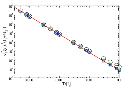
The data collapse onto the analytical curve is perfect over temperatures of several orders of magnitude. We note that the closer $\tilde{\alpha}$ is to the critical point QCP1 the lower the temperatures are where the universal scaling sets in.

Similarly, we can also check the formula for the critical point, $\tilde{\alpha}=-4$, see Fig. 3.

Figure 3: (Color online) Analytical formula (9) for the low-temperature susceptibility at $\tilde{\alpha}=-4$ (line) compared to MC data (circles).

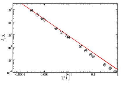
The numerical data do confirm the analytical result, however, we note that temperatures $T/|J_{1}|\ll 0.01$ are required.

IV The quantum model

The quantum $s=1/2$ nearest-neighbor ($J_{2}=0$) ferromagnetic Heisenberg chain is exactly solvable. Thermodynamic properties, in particular the susceptibility, have been calculated using the thermodynamic Bethe ansatz.Takahashi (1986, 1987a) The results have been shown to be in excellent agreement with those obtained by a modified spin-wave theory (MSWT).Takahashi (1987a) In the following we extend the MSWT approach to the ferromagnetic phase of the $J_{1}$-$J_{2}$ model and to the quantum critical point. We then test the obtained analytical results by comparing with numerical data obtained by the transfer matrix renormalization group.Bursill et al. (1996); Wang and Xiang (1997); Sirker and Klümper (2002a, b); Sirker (2010)

IV.1 Modified spin wave theory

To calculate the thermodynamic properties of the spin-$s$ ferromagnetic Heisenberg chain, Takahashi [Takahashi, 1987a, 1986] introduced a modified spin-wave theory. The spin operators are represented by bosonic operators as in regular spin-wave theory. In addition, the constraint of vanishing magnetization at finite temperatures posed by the Mermin-Wagner theorem is implemented in a simple way by adding an effective magnetic field which acts as a Lagrange multiplier for the magnetization. MSWT has also been used successfully to describe boundary contributions in the open ferromagnetic Heisenberg chain Sirker and Bortz (2006) as well as the thermodynamics in the dimerized ferromagnet.Sirker et al. (2008); Herzog et al. (2010, 2011) Moreover it has been shown that the classical ferromagnetic chain is well-described by MSWT.Takahashi (1987a); Sirker and Bortz (2006); Takahashi (1987b) Here we will apply the same method to the Hamiltonian (1) with general spin $s$.

We expect that MSWT can be applied for $\tilde{\alpha}<-4$ where the ground state is ferromagnetic. We will also use this approximation for the QCP at $\tilde{\alpha}=-4$, however, here the validity of MSWT is questionable because of the degeneracy of the ferromagnetic ground state with RVB states. A further discussion will be presented in Sec. IV.2, based on a comparison with numerical data, and in the conclusions, Sec. V. In the MSWT approximation the Hamiltonian (1) is represented as (in the following we set the lattice constant $a_{0}=1$)

$$H=N(J_{1}+J_{2})s^{2}+\sum_{k}\omega_{k}a^{\dagger}_{k}a_{k}$$ (10)

where $a_{k}^{(\dagger)}$ is a bosonic annihilation (creation) operator with $[a_{k},a_{k^{\prime}}^{\dagger}]=\delta_{k,k^{\prime}}$. The dispersion relation is given by $\omega_{k}=2s(|J_{1}|\left[1-\cos k\right]+J_{2}\left[\cos(2k)-1\right])$. The additional constraint of vanishing magnetization reads $s=N^{-1}\sum_{k}n_{k}$ where $n_{k}=(\exp[\omega_{k}/T+v]-1)^{-1}$ is the Bose function including the effective magnetic field, $v\equiv h/T$.

First, we study the case $\tilde{\alpha}<-4$. For small temperatures only spin-wave excitations with small momenta contribute and the dispersion can be approximated as $\omega_{k}=|J_{1}|s(1-4/|\tilde{\alpha}|)k^{2}$. The constraint can now be solved explicitly by expanding in the reduced temperature $t$. This leads to

$$\sqrt{v} = \frac{\sqrt{t}}{2s}\left(1+\frac{\zeta(\frac{1}{2})}{\sqrt{\pi}}\frac{\sqrt{t}}{2s}+\frac{\zeta^{2}(\frac{1}{2})}{\pi}\left(\frac{\sqrt{t}}{2s}\right)^{2}+\dots\right),$$

$$t \equiv \frac{T}{|J_{1}|s(1-4/|\tilde{\alpha}|)}.$$ (11)

Here $\zeta(x)$ is the Riemann zeta-function. We note that the expression for $v$ is the same as for the simple ferromagnet,Takahashi (1987a) only the definition of the reduced temperature is modified. The expansion (IV.1) is valid if $\sqrt{t}/2s\ll 1$, i.e., the temperature range where this result is applicable shrinks the closer we get to the critical point. The free energy in spin-wave approximation is given by

$$f=(J_{1}+J_{2})s^{2}-T\left[vs+\frac{1}{N}\sum_{k}\ln(1+n_{k})\right]\,.$$ (12)

At small temperatures we can expand the second term in $v$ and obtain

$$f=(J_{1}+J_{2})s^{2}-T\left[\frac{\zeta(3/2)}{2}\sqrt{\frac{t}{\pi}}-\frac{t}{4s}+\cdots\right]\,.$$ (13)

In agreement with the scaling relations derived in Sec. II we find as leading temperature dependence $f\sim-T^{3/2}$. From $C=-T\partial^{2}f/\partial T^{2}$ the leading temperature dependence of the specific heat can be obtained.

The susceptibility in MSWT is given by

$$\chi=\frac{1}{3TN}\sum_{k}n_{k}(n_{k}+1)$$ (14)

leading to the low-temperature expansion

$$\chi=\frac{s^{3}}{T}\left[\frac{2}{3t}-\frac{\zeta(\frac{1}{2})}{\sqrt{\pi s^{2}t}}+\dots\right]\,.$$ (15)

The leading temperature dependence found in MSWT therefore agrees exactly with formula (7) found by general scaling arguments.

Next, we consider the critical point $\tilde{\alpha}=-4$. For small momenta the dispersion now reads $\omega_{k}=|J_{1}|sk^{4}/4$ and thus the dispersion changes from quadratic to quartic which will have consequences for the temperature scaling of thermodynamic quantities. For the constraint we find

$$v=\left(\frac{\tilde{t}}{64s^{4}}\right)^{1/3}\left[1+\frac{\sqrt{2}\zeta(1/4)}{3s\Gamma(3/4)}\tilde{t}^{1/4}+\cdots\right]$$ (16)

with a new reduced temperature $\tilde{t}\equiv 4T/(|J_{1}|s)$. Using relation (12) we obtain for the free energy

$$f=(J_{1}+J_{2})s^{2}-T\left[\frac{\Gamma(1/4)\zeta(5/4)}{4\pi}\tilde{t}^{1/4}-3\left(\frac{\tilde{t}}{64s}\right)^{1/3}\right]$$ (17)

plus higher order terms. The scaling of the leading term, $f\sim-T^{5/4}$, is again consistent with the scaling arguments in Sec. II. Finally, we can calculate the susceptibility using Eq. (14) and obtain

$$\chi=\frac{1}{T}\left[\left(\frac{s^{7}}{\tilde{t}}\right)^{1/3}-\frac{7\zeta(\frac{1}{4})s^{4/3}}{6\sqrt{2}\Gamma(\frac{3}{4})}\left(\frac{1}{\tilde{t}}\right)^{1/12}+\frac{S}{3}+\dots\right]$$ (18)

We note that the scaling of the leading term is the same as in Eq. (9). However, the numerical prefactor is not the same. For the case $s=1/2$ we find, in particular, from (18) that $\chi=2^{-10/3}T^{-4/3}\approx 0.0992\,T^{-4/3}$. In contrast, Eq. (9)—which does give the correct low-temperature behavior of the classical model, see Fig. 3—yields $\chi\approx 0.1685\,T^{-4/3}$. First of all, this does suggest that at the QCP the classical and the quantum model no longer show the same thermodynamic properties at low temperatures. However, similarly to the scaling approach used in Sec. II one might also question the foundations of MSWT for the QCP alltogether. At the QCP the ground state is no longer a simple ferromagnet suggesting that also the excitations are no longer described by simple spin waves. Furthermore, UV divergencies in contributions from spin wave interaction terms might be expected because we are now dealing with a theory above the upper critical dimension. An independent test of the scaling and the MSWT approach at the QCP can only be obtained by unbiased numerical calculations. Such calculations will be presented in the next subsection.

IV.2 Numerical results

The quantum critical point QCP1 at $\tilde{\alpha}=-4$ is characterized by a level crossing of a singlet and a fully polarized state. Right at the critical point the singlet-triplet gap $\Delta_{st}$ is therefore expected to vanish. This is confirmed by the Lanczos calculations for finite size chains shown in Fig. 4.

Figure 4: (Color online) Numerical data (squares) for the singlet-triplet gap $\Delta_{st}$ for chains of even lengths $N=12,14,\cdots,36$. The solid line is a fit $\Delta_{st}=a_{0}+a_{1}\left(N^{-5}\right)^{a_{2}}$ with $a_{0}=-4.8\cdot 10^{-7}$, $a_{1}=594.1$, and $a_{2}=0.9994$.

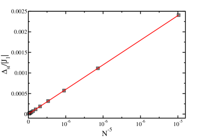
We find, in particular, that the singlet-triplet gap vanishes as $\Delta_{st}\sim N^{-5}$.

The thermodynamics of the $J_{1}-J_{2}$ model has been studied previously by a Green’s function methodHärtel et al. (2008) and by TMRG.Sirker (2010) In the second approach the one-dimensional quantum model is mapped onto a two-dimensional classical model with the help of a Trotter-Suzuki decomposition. It is then possible to express the partition function in terms of a transfer matrix for the classical model with the free energy depending only on the largest eigenvalue of this transfer matrix. The transfer matrix is extended in imaginary time direction—corresponding to a successive lowering of the temperature—with the help of a density-matrix renormalization group algorithm. For details concerning the algorithm the reader is referred to Refs. [I.Peschel et al., 1999; Bursill et al., 1996; Wang and Xiang, 1997; Shibata, 1997; Sirker and Klümper, 2002b, a].

Here we want to use the TMRG algorithm to test in how far the analytical predictions from the previous section hold for the $s=1/2$ case. In Fig. 5 numerical data for the susceptibility are compared to MSWT for $\tilde{\alpha}=-20$.

Figure 5: (Color online) Susceptibility for $\tilde{\alpha}=-20$. The symbols denote the TMRG data, the solid line a solution of (14) where the Lagrange parameter $v$ is determined by solving the non-linear equations numerically, and the dashed line the leading low-temperature asymptotics (15) extracted analytically. The inset shows the low-temperature region on a logarithmic scale.

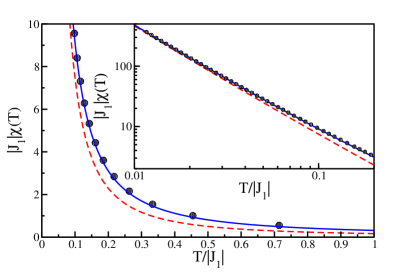
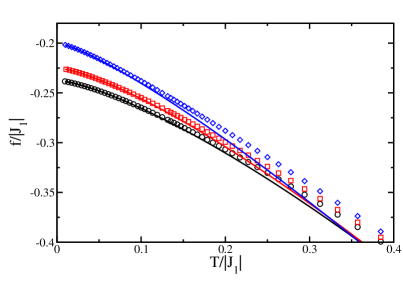
If we numerically solve the non-linear equation for the Lagrange parameter $v$ then the MSWT prediction is in excellent agreement with the numerical data up to temperatures of order $t/s\sim 1$. The formula (14) makes use of a representation of the susceptibility in terms of the spin-spin correlation function $\langle\boldsymbol{S}_{i}\boldsymbol{S}_{j}\rangle$ which also includes terms quartic in the bosonic operators. In this case, the constraint fortunately makes it possible to obtain a final expression which is still only bilinear in the bosonic operators. The result presented in Fig. 5 therefore goes beyond linear spin-wave theory. The formula for the free energy, Eq. (12), is, however, a linear spin-wave expression. Here it is not possible to include the quartic terms without further approximations because the constraint alone is not sufficient to obtain a final expression which is only bilinear in the bosonic operators. The MSWT results for the free energy are therefore only valid at very low temperatures as can be seen by the comparison with numerical data, Fig. 6.

Figure 6: (Color online) The free energy for $\tilde{\alpha}=-20,-10,-5$ (from bottom to top). The symbols denote the TMRG data, the solid lines the MSWT result (12) using a fully self-consistent solution for the Lagrange parameter $v$.

A similar comparison for the critical point is shown in Fig. 7.

Figure 7: (Color online) Free energy for the critical point $\tilde{\alpha}=-4$. The symbols denote the TMRG data, the dashed line the leading terms in the low-temperature asymptotics (17) obtained by MSWT. The solid line represents the fully self-consistent solution of Eq. (12).

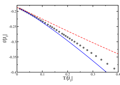
There is good quantitative agreement at temperatures $\tilde{t}/s\lesssim 1$, i.e. $T/|J_{1}|\lesssim 0.0625$ between the numerics and the fully self-consistent solution of the MSWT equations.

For the susceptibility the situation is expected to be more complex. The scaling hypothesis used to derive Eq. (9) is questionable because at the critical point we are above the upper critical dimension. Indeed, we have already seen that the predictions from MSWT deviate from formula (9) which we have confirmed to be the correct result for the classical model. This is contrary to the ferromagnetic regime where the MSWT results coincide at low temperatures with the solution of the classical model. A comparison with numerical data, Fig. 8, indicates nevertheless an apparently good quantitative agreement with MSWT up to temperatures $T\sim|J_{1}|$.

Figure 8: (Color online) Susceptibility for the critical point $\tilde{\alpha}=-4$. (a) and (b): The symbols denote the TMRG data, the solid line a solution of (14) where the Lagrange parameter $v$ is determined self-consistently, and the dashed line the low-temperature asymptotics (18). The inset (b) shows the low-temperature region on a logarithmic scale. (c) Comparison between numerical data for the quantum model (small circles) and the classical model (squares).

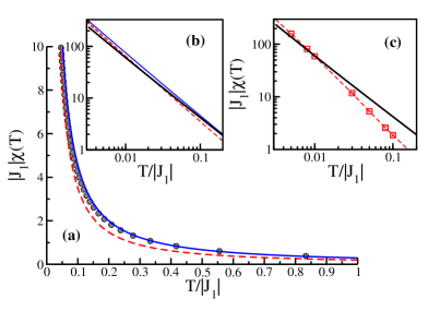
A closer inspection of the low-temperature asymptotics (see inset (b) of Fig. 8), however, shows that MSWT is not fully consistent with the numerics. Furthermore, inset (c) shows that classical and quantum model no longer share the same low-temperature properties. If we fit the numerically obtained $\chi(T)$ for the quantum model to a simple power law and vary the fit region we obtain the values summarized in table 1.

$T_{\rm max}$	$A$	$\gamma$
0.05	0.245	1.195
0.025	0.259	1.185
0.01	0.247	1.193
0.0075	0.244	1.195
0.005	0.240	1.198
0.004	0.237	1.201

Table 1: Parameters obtained by fitting $\chi(T)$ in Fig. 8 to $\chi(T)=A\cdot T^{-\gamma}$ in the interval $T/|J_{1}|\in[0.003,T_{\rm max}]$.

This seems to indicate that the exponent might actually be smaller than $4/3$ and therefore different from the exponent in the classical model. However, using the TMRG algorithm we are not able to reach temperatures for the quantum model which are as low as those obtainable for the classical model using MC simulations. We therefore can not completely rule out that the temperatures are just not low enough to observe the $T^{-4/3}$ power law predicted by MSWT.

V Conclusions

In summary, we have studied the frustrated $J_{1}$-$J_{2}$ Heisenberg chain at and near to its $z=4$ critical point at $\tilde{\alpha}=J_{1}/J_{2}=-4$. By developing a field theory we have discussed how the system is driven from a ferromagnetic state to a state with incommensurate (spiral) spin-spin correlations. Based on this analysis, the classical and the quantum model are expected to show the same low-energy properties in the ferromagnetic phase.

From scaling arguments we obtained, in particular, that the susceptibility diverges $\chi\sim(J_{1}+4J_{2})/T^{2}$ in the ferromagnetic phase with a known proportionality constant. We could reproduce this result using an alternative analytical approach based on a modified spin wave theory. Furthermore, we have verified the analytical prediction using Monte Carlo simulations for the classical model and the transfer matrix renormalization group for the quantum model and have found excellent agreement.

Right at the critical point, $J_{1}/J_{2}=-4$, simple dimensional analysis allowed us to predict the scaling of the free energy and specific heat with temperature. In particular, we found that the free energy scales as $f\sim T^{5/4}$. Our modified spin wave theory calculations have confirmed this scaling and the obtained parameter-free results have been shown to be in good agreement with numerical data for the quantum model at low temperatures. Scaling arguments can also be used to obtain a parameter-free formula for the low-temperature behavior of the susceptibility, which—according to this formula—diverges as $\chi\sim T^{-4/3}$. From the field theory analysis even the prefactor can be obtained and we have shown, using Monte-Carlo simulations, that this formula is indeed correct for the classical model.

The most interesting problem is the temperature dependence of the susceptibility at the critical point $J_{1}/J_{2}=-4$ for the quantum model. The modified spin wave approach also yields a $T^{-4/3}$ divergence, however, the prefactor is different from the one obtained from field theory. The numerical data, furthermore, seem to indicate that even the exponent might deviate from $4/3$. From fits of our numerical data at the lowest accessible temperatures we have obtained $\chi\sim T^{-1.2}$.

There are a number of possible reasons for this deviation: The simplest explanation is that we do not have numerical data for low enough temperatures to observe the true scaling behavior. However, there are good reasons to believe that the observed deviation has physical reasons. An inspection of the quartic term describing the interaction of spin waves within spin wave theory shows that this term is ultraviolet divergent. Such divergences are expected because $d+z=5$ is larger than the upper critical dimension. In such a case the ultraviolet properties of the theory can affect the critical behavior.

Another problem is the treatment of the Berry phase term which we have ignored in our field theory analysis. On the basis of a bosonization approach,Nersesyan et al. (1998); Itoi and Qin (2001) where the system is considered starting from the decoupling point $\tilde{\alpha}=0$, the spiral phase of the quantum model has been found to be gapped. Since we do not expect an additional phase transition, a gap should exist all the way to $\tilde{\alpha}\to-4$. In the field theory approach this gap in the quantum model must be related to the Berry phase term. This term might therefore also be important for the physical properties right at the transition point. This expectation seems to be consistent both with the known degeneracy of the ferromagnetic and resonance valence bond states at this point and our numerical results which show that the low-temperature properties of the classical and the quantum model are different.

The results attained here might be relevant and should be compared to future experiments on edge-sharing cuprate chain compounds.