Standard model with compactified spatial dimensions

Abstract

We analyze the structure of the standard model coupled to gravity with spatial dimensions compactified on a three-torus. We find that there are no stable one-dimensional vacua at zero temperature, although there does exist an unstable vacuum for a particular set of Dirac neutrino masses.

I Introduction

The standard model coupled to gravity has a unique four-dimensional vacuum. Nevertheless, in case of one spatial dimension compactified on a circle Arkani , or for two spatial dimensions compactified on a 2-torus, it has recently been shown that there may also exist lower-dimensional vacua stabilized by the Casimir energies of the standard model particles with the lowest mass, i.e., gravitons, photons and neutrinos. Such vacua of the low-energy effective theory exist at zero temperature for a wide range of experimentally allowed neutrino masses. In AFI it was shown that at high enough temperatures these stationary points are washed out. At zero temperature an extremely small rate for tunneling to a lower-dimensional anti-de Sitter spacetime was found following the steps outlined in Sean .

This work completes the series of papers Arkani ; AFW ; AFI concerning lower-dimensional standard model vacua by considering the last remaining case, when all spatial dimensions are compactified. We analyze the compactifications on $T^{3}$, $S^{1}\times S^{1}\times S^{1}$, $S^{1}\times T^{2}$, $S^{3}$, and $S^{1}\times S^{2}$, but our primary focus is on the 3-torus case, since it seems the most natural three-dimensional topology with no curvature.

Three-dimensional compactifications are qualitatively different from the one- and two-dimensional compactifications, since a stable vacuum cannot occur for a “generic range” of neutrino masses. Nonetheless, a brief study of this case is worthwhile. The geometry of the lower-dimensional vacuum is determined by the shape of the effective potential, which is a sum of Casimir energies of the particles and the cosmological constant term. We show that this potential for the 3-torus case has no stable stationary points at zero temperature. For the standard model with Dirac neutrinos, however, there does exist an unstable stationary point for a particular set of neutrino masses, depending on the type of hierarchy.

II Compactification on a 3-torus at zero temperature

In this section we explore the existence of lower-dimensional vacua of the standard model coupled to gravity with spatial dimensions compactified on a 3-torus. We start with the 4D Einstein-Hilbert action,

$$S=\int d^{4}x\sqrt{-g}\left[\frac{1}{2}M_{p}^{2}{\cal R}+\mathcal{L}_{\rm SM}\right],$$ (1)

where $g$ is the determinant of the 4D metric, the Planck mass $M_{p}\simeq 2.4\times 10^{18}~{}{\rm GeV}$, $\mathcal{R}$ is the Ricci scalar, and $\mathcal{L}_{\rm SM}$ is the standard model Lagrangian including the cosmological constant. Consider the following spacetime interval,

$$ds^{2}=-N^{2}dt^{2}+T_{ij}dy^{i}dy^{j}\,,$$ (2)

where $T_{ij}$ is the metric on the 3-torus with $i,j=1,2,3$ and the compact coordinates $y^{i}\in[0,2\pi)$. We adopt the same parametrization as in Arkani ,

$$T_{ij}=\frac{b^{2}}{(\rho_{3}\tau_{2})^{2/3}}\left(\begin{array}[]{ccc}1&\tau_{1}&\rho_{1}\\ \tau_{1}&\tau_{1}^{2}+\tau_{2}^{2}&\rho_{1}\tau_{1}+\rho_{2}\tau_{2}\\ \rho_{1}&\rho_{1}\tau_{1}+\rho_{2}\tau_{2}&\rho_{1}^{2}+\rho_{2}^{2}+\rho_{3}^{2}\\ \end{array}\right),$$ (6)

where $\Psi^{\rm T}=(\tau_{1},\tau_{2},\rho_{1},\rho_{2},\rho_{3})$ are the shape moduli and $b^{3}$ is the volume modulus, all functions only of time. The dimensionally reduced action is,

$$S=\!\!\int\!dt\!\left[\frac{1}{2}M_{p}^{2}\frac{(2\pi b)^{3}}{N}\left(\!-6\,\frac{\dot{b}^{2}}{b^{2}}\!+\!\dot{\Psi}^{\rm T}\hat{M}\dot{\Psi}\!\right)\!-\!N\,V(b,\Psi)\!\right]$$ (7)

where the dot indicates a derivative with respect to time. The potential is given by,

$$V(b,\Psi)=(2\pi b)^{3}\Lambda+\!\!\sum_{\rm particles}\!\!N_{f}\,E_{0}(b,\Psi,m)\ ,$$ (8)

where $\Lambda$ is the cosmological constant, $E_{0}$ is the Casimir energy for a scalar of mass $m$, and $N_{f}$ is the number of degrees of freedom, with a positive sign for bosons and a negative sign for fermions (i.e., $N_{f}=2$ for the photon and graviton, $N_{f}=-4$ for a Dirac neutrino, $N_{f}=-2$ for a Majorana neutrino Arkani ; Ponton ; Rubin ). In formula (7) the matrix $\hat{M}$ has the following nonzero entries,

$$M_{11}=\frac{\rho_{2}^{2}+\rho_{3}^{2}}{2\tau_{2}^{2}\rho_{3}^{2}}\ ,\ \ M_{22}=\frac{3\rho_{2}^{2}+4\rho_{3}^{2}}{6\tau_{2}^{2}\rho_{3}^{2}}\ ,\ \ M_{55}=\frac{2}{3\rho_{3}^{2}}\ ,$$

$$M_{25}=M_{52}=-\frac{1}{3\tau_{2}\rho_{3}}\ ,\ \ M_{33}=M_{44}=\frac{1}{2\rho_{3}^{2}}\ ,$$

$$M_{13}=M_{31}=M_{24}=M_{42}=\frac{\rho_{2}}{2\tau_{2}\rho_{3}^{2}}\ .$$ (9)

It is easy to check that $\hat{M}$ is positive definite. Varying the action (7) with respect to $N$ and setting $N=1$ (which corresponds to fixing the gauge) we arrive at,

$$\frac{1}{2}M_{p}^{2}(2\pi)^{3}\left(-6\,b\,\dot{b}^{2}+b^{3}\,\dot{\Psi}^{\rm T}\hat{M}\dot{\Psi}\right)+V(b,\Psi)=0\ ,$$ (10)

thus the total energy has to vanish. As a consequence, the existence of a vacuum at $(b_{0},\Psi_{0})$ requires $V(b_{0},\Psi_{0})=0$. In addition, we can set $N=1$ directly in the action (7) and write down the equations of motion that arise from varying the action with respect to the other parameters. For the volume modulus it takes the form,

$$\frac{\ddot{b}}{b}+\frac{1}{2}\frac{\dot{b}^{2}}{b^{2}}+\frac{1}{4}\dot{\Psi}^{\rm T}\hat{M}\dot{\Psi}-\frac{1}{48\pi^{3}M_{p}^{2}b^{2}}\frac{\partial V(b,\Psi)}{\partial b}=0\ .$$ (11)

As noted in Arkani , since all shape moduli have positive definite kinetic energy, while for the volume modulus it is negative, the conditions for the existence of a stable vacuum are,

$$V=0\ ,\ \ \partial_{b}V=\partial_{\alpha}V=0\ ,\ \ \partial_{b}^{2}V<0\ ,\ \ \partial_{\alpha}^{2}V>0$$ (12)

at the stationary point, where $\alpha=\tau_{1},\tau_{2},\rho_{1},\rho_{2},\rho_{3}$. This presents a fine tuning problem since both the potential and its derivative have to vanish at the same point. In addition, as we will shortly show, even conditions (12) themselves cannot be fulfilled simultaneously.

Note that the potential $V(b,\Psi)$ is expressed in terms of bare quantities, each of which is divergent. We first write the cosmological constant as,

$$\Lambda=\Lambda^{\rm obs}+\Lambda^{\rm div}\ ,$$ (13)

where $\Lambda^{\rm obs}\simeq 3.1\times 10^{-47}~{}{\rm GeV}^{4}$ pdg is the observed value, and $\Lambda^{\rm div}$ is the divergent quantum correction, equal to the sum of Casimir energies of particles in flat space,

$$\Lambda^{\rm div}=\frac{\Gamma\left(-2\right)}{32\,\pi^{2}}\sum_{\rm particles}N_{f}\,m^{4}\ .$$ (14)

The Casimir energy for a scalar of mass $m$ in a 4D spacetime with spatial dimensions compactified on a 3-torus, assuming periodic boundary conditions, is,

$$E_{0}(b,\Psi,m)=\frac{1}{2}\sum_{n_{1},n_{2},n_{3}=-\infty}^{\infty}\left(T^{ij}n_{i}n_{j}+m^{2}\right)^{\frac{1}{2}},$$ (15)

where $T^{ij}$ is the inverse of $T_{ij}$ given by equation (6). The regularized expression for the triple sum in (15) is derived in the appendix. We immediately notice that the divergent parts in formula (8) cancel and we can write the potential as,

$$V(b,\Psi)=(2\pi b)^{3}\Lambda^{\rm obs}+\!\!\sum_{\rm particles}N_{f}\,E_{0}^{\rm obs}(b,\Psi,m)\ ,$$ (16)

where the finite part of the Casimir energy (15) is given by,

$$\,E_{0}^{\rm obs}(b,\Psi,m)=-\frac{1}{\pi}\frac{1}{\sqrt{T^{11}}}\Bigg{\{}m\,\sqrt{T^{11}}\sum_{n=1}^{\infty}\frac{1}{n}\,K_{1}\!\left(\tfrac{2\pi m}{\sqrt{T^{11}}}n\right)$$ (17)

$$\!+\,\sqrt{T^{11}}\!\!\!\!\!\!\sum_{n_{2},n_{3}=-\infty}^{\infty}\!\!\!\!\!\!\!{}^{\prime}\ \ \ \,\sum_{n_{1}=1}^{\infty}\frac{1}{n_{1}}\cos\Big{[}\tfrac{2\pi}{T^{11}}n_{1}(n_{2}T^{12}+n_{3}T^{13})\Big{]}$$

$$\ \ \,\times\,\sqrt{d(n_{2},n_{3})+m^{2}}\,\,\,K_{1}\!\left[\tfrac{2\pi}{\sqrt{T^{11}}}n_{1}\sqrt{d(n_{2},n_{3})+m^{2}}\right]$$

$$\!+\,\,m^{3/2}\,\Delta_{11}^{1/4}\sum_{n=1}^{\infty}\frac{1}{n^{3/2}}\,K_{3/2}\!\left(\tfrac{2\pi\,m}{\sqrt{\Delta_{11}}}\,n\right)$$

$$\!+\,\,m^{2}\,\sqrt{\frac{D^{\prime}}{\Delta_{11}}}\,\sum_{n=1}^{\infty}\frac{1}{n^{2}}\,K_{2}\!\left(\tfrac{2\pi\,m}{\sqrt{D^{\prime}}}\,n\right)$$

$$\!+\,2\,\Delta_{11}^{1/4}\!\!\sum_{n_{2},n_{3}=1}^{\infty}\left(D^{\prime}n_{3}^{2}+m^{2}\right)^{3/4}\cos\left[2\,\pi\,n_{2}\,n_{3}\tfrac{\Delta_{12}}{\Delta_{11}}\right]$$

$$\ \ \,\times\,\frac{1}{n^{3/2}_{2}}\,K_{3/2}\!\left(\tfrac{2\pi}{\sqrt{\Delta_{11}}}n_{2}\sqrt{D^{\prime}n_{3}^{2}+m^{2}}\right)\Bigg{\}}\ .$$

In formula (17), $K_{n}(x)$ is the modified Bessel function of the second kind, the matrix $\hat{\Delta}$ and function $d$ are,

$$\!\!\hat{\Delta}=\frac{1}{T^{11}}\Bigg{(}\!\begin{array}[]{cc}T^{11}T^{22}-(T^{12})^{2}&\ T^{11}T^{23}-T^{12}T^{13}\\ T^{11}T^{23}-T^{12}T^{13}&\ T^{11}T^{33}-(T^{13})^{2}\\ \end{array}\!\Bigg{)},$$ (20)

$$d(n_{2},n_{3})=\left(\!\begin{array}[]{cc}n_{2}&n_{3}\\ \end{array}\!\right)\hat{\Delta}\left(\!\begin{array}[]{c}n_{2}\\ n_{3}\\ \end{array}\!\right),$$ (24)

and $D^{\prime}=\det(\hat{\Delta})/\Delta_{11}$. In the massless limit formula (17) reduces to,

$$\ E_{0}^{\rm obs}(b,\Psi,0)\ =\ -\frac{1}{\pi}\frac{1}{\sqrt{T^{11}}}\ \Bigg{\{}\frac{\pi}{12}\ T^{11}$$ (25)

$$\!+\,\sqrt{T^{11}}\!\!\!\!\!\!\sum_{n_{2},n_{3}=-\infty}^{\infty}\!\!\!\!\!\!\!{}^{\prime}\ \ \ \,\sum_{n_{1}=1}^{\infty}\frac{1}{n_{1}}\cos\Big{[}\tfrac{2\pi}{T^{11}}n_{1}(n_{2}T^{12}+n_{3}T^{13})\Big{]}$$

$$\ \ \,\times\,\sqrt{d(n_{2},n_{3})}\,\,\,K_{1}\!\left[\tfrac{2\pi}{\sqrt{T^{11}}}n_{1}\sqrt{d(n_{2},n_{3})}\right]$$

$$\!+\,\frac{\zeta(3)}{4\pi}\Delta_{11}+\frac{\pi^{2}}{180}\frac{1}{\sqrt{\Delta_{11}}}D^{\prime\ 3/2}$$

$$\!+\,2\,\Delta_{11}^{1/4}\,D^{\prime\ 3/4}\sum_{n_{2},n_{3}=1}^{\infty}\cos\left[2\,\pi\,n_{2}\,n_{3}\tfrac{\Delta_{12}}{\Delta_{11}}\right]$$

$$\,\ \ \times\,\left(\frac{n_{3}}{n_{2}}\right)^{3/2}K_{3/2}\!\left(2\,\pi\,n_{2}\,n_{3}\,\sqrt{\tfrac{D^{\prime}}{\Delta_{11}}}\right)\Bigg{\}}\ .$$

Note that for $m\gg 1/b$ the Casimir energy (17) behaves like $\exp(-C\,b\,m)$, where $C$ is a constant and depends on the shape moduli. We restrict our attention to the lengthscale $b\gg 1/m_{e}$, so that the Casimir energies of the electron and all heavier standard model particles are negligible compared to the contributions of the photon, graviton, and neutrinos.

It turns out that even before performing the numerical analysis, we can precisely determine the values of the shape moduli for which the potential (16) has its extrema. It can be shown that the Casimir energy (15) is invariant under $\textrm{SL}(3,\mathbb{Z})$ transformations. The nine generators of the $\textrm{SL}(3,\mathbb{Z})$ group are listed in SL3 ; generators . For example, the generator $T_{1}:\tau_{1}\rightarrow\tau_{1}+1$ corresponds to a change of indices $(n_{1},n_{2},n_{3})\rightarrow(n_{1},n_{2}-n_{1},n_{3})$ in (15), whereas $T_{3}:\rho_{3}\rightarrow\rho_{3}+1$ is equivalent to replacing $(n_{1},n_{2},n_{3})\rightarrow(n_{1},n_{2},n_{3}-n_{1})$. The same symmetries are exhibited by the potential (16), since it is a linear combination of Casimir energies of the particles. It has been argued that fixed points of the transformation under which the potential is invariant correspond to extrema of this potential 6D4 ; Ponton ; Wilczek . Such fixed points should also lie on the boundary of the fundamental domain of the symmetry group. The fundamental region for a 3-torus parametrized as in (6) is the following SL3 ; fund ,

$$\!\!\!\!\!\!\!\!1\leq\tau_{1}^{2}+\tau_{2}^{2}\leq\rho_{1}^{2}+\rho_{2}^{2}+\rho_{3}^{2}\ ,\ \ \ -1/2<\rho_{1},\tau_{1}\leq 1/2\ ,$$

$$\ \ \rho_{1}\tau_{1}+\rho_{2}\tau_{2}\leq(\tau_{1}^{2}+\tau_{2}^{2})/2\ ,\ \ \ \ \ \ \tau_{2}>0\ .$$ (26)

This is the moduli space of physically distinct 3-tori. Fixed points of $\textrm{SL}(3,\mathbb{Z})$ correspond to the case when the inequalities in the first and third relation in (II) become equalities, while $\tau_{1},\rho_{1}$ are $0$ or $1/2$. A numerical analysis shows that the fixed point corresponding to a minimum of the potential exists for $\tau_{1}=\rho_{1}=1/2$, thus the shape moduli for a vacuum stable in the subspace $\left(\tau_{1},\tau_{2},\rho_{1},\rho_{2},\rho_{3}\right)$ are,

$$\Psi_{0}^{\rm T}=\left(\frac{1}{2},\frac{\sqrt{3}}{2},\frac{1}{2},\frac{\sqrt{3}}{6},\frac{\sqrt{6}}{3}\right)\ .$$ (27)

Although neutrino masses have not been determined, we can use experimental mass splittings for the atmospheric and solar neutrinos to generate the spectrum given the lightest neutrino mass and a choice of hierarchy. This allows us to investigate the potential for various lightest neutrino masses. Experimentally, $\Delta m^{2}_{\rm atm}=(2.43\pm 0.13)\times 10^{-3}{\ \rm eV^{2}}$, $\Delta m^{2}_{\rm sol}=(7.59\pm 0.20)\times 10^{-5}{\ \rm eV^{2}}$ pdg . Denoting the lightest neutrino mass by $m_{l}$, the masses of the other two neutrinos, assuming normal hierarchy, are $m_{l}^{2}+\Delta m^{2}_{\rm sol}$ and $m_{l}^{2}+\Delta m^{2}_{\rm atm}+\Delta m^{2}_{\rm sol}$, whereas for an inverted hierarchy the masses are $m_{l}^{2}+\Delta m^{2}_{\rm atm}-\Delta m^{2}_{\rm sol}$ and $m_{l}^{2}+\Delta m^{2}_{\rm atm}$.

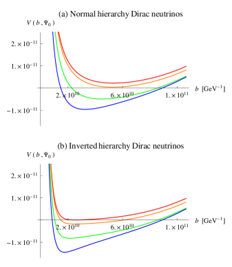
Figure 1: (a) Plots of $V(b,\Psi_{0})$ for Dirac neutrinos with normal hierarchy for masses $m_{l}=0$ (red), $10^{-12}\ {\rm GeV}$ (orange), $5\times 10^{-12}\ {\rm GeV}$ (green), and $10^{-11}\ {\rm GeV}$ (blue). (b) The same for an inverted hierarchy.

Under our assumption $b\gg 1/m_{e}$, the potential in case of the standard model with Dirac neutrinos is,

$$\!\!\!\!V(b,\Psi_{0})=(2\pi b)^{3}\Lambda^{\rm obs}$$ (28)

$$+\bigg{[}\,4\,E^{\rm obs}(b,\Psi_{0},0)-\,4\,\sum_{i=1}^{3}E^{\rm obs}(b,\Psi_{0},m_{\nu_{i}})\bigg{]}.$$

The plots of $V(b,\Psi_{0})$ for several lightest neutrino masses for normal and inverted hierarchy Dirac neutrinos are given in figure 1 (a) and (b), respectively. The only extremum of the potential is a minimum, but the conditions for a stable stationary point (12) require it to be a maximum. This proves that there are no stable one-dimensional vacua of the low-energy effective theory. Nevertheless, we find precisely one set of neutrino masses for each type of hierarchy for which an unstable vacuum exists. In the case of normal hierarchy Dirac neutrinos the lightest neutrino mass for such an unstable vacuum is $m_{l}\approx 10^{-12}{\rm\ GeV}$, whereas in the inverted hierarchy case it is $m_{l}\approx 0$. Both unstable vacua appear at the micron scale.

In the case of the standard model with Majorana neutrinos the potential takes the form,

$$\!\!\!\!V(b,\Psi_{0})=(2\pi b)^{3}\Lambda^{\rm obs}$$ (29)

$$+\bigg{[}\,4\,E^{\rm obs}(b,\Psi_{0},0)-\,2\,\sum_{i=1}^{3}E^{\rm obs}(b,\Psi_{0},m_{\nu_{i}})\bigg{]}.$$

Figure 2 (a) and (b) shows the plot of $V(b,\Psi_{0})$ for Majorana neutrinos for a few lightest neutrino masses. Note that in this case there does not even exist an unstable vacuum.

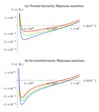
Figure 2: Plots of $V(b,\Psi_{0})$ for Majorana neutrinos with normal hierarchy (figure (a)) and inverted hierarchy (figure (b)) for masses $m_{l}=0$ (red), $10^{-12}\ {\rm GeV}$ (orange), $5\times 10^{-12}\ {\rm GeV}$ (green), and $10^{-11}\ {\rm GeV}$ (blue).

III Compactifications on other 3D manifolds

Our analysis from the last section can be easily extended to other topologies of the compact space, for instance $S^{1}\times S^{1}\times S^{1}$, $S^{1}\times T^{2}$, $S^{3}$, and $S^{1}\times S^{2}$. The first two cases are very similar to $T^{3}$. We briefly comment on the other two possibilities, which are considerably different because of a nonzero curvature of the compact space.

III.1 Compactification on $S^{1}\times S^{1}\times S^{1}$

Denoting the radii of compactification by $R_{1},R_{2},R_{3}$, the metric takes the form,

$$\!\!\!ds^{2}=-N^{2}dt^{2}+R_{1}^{2}(dy^{1})^{2}+R_{2}^{2}(dy^{2})^{2}+R_{3}^{2}(dy^{3})^{2},$$ (30)

where  $y^{1},y^{2},y^{3}\in[0,2\pi)$. The dimensionally reduced action (1) is,

$$S=\!\int\!dt\left[\frac{1}{2}M_{p}^{2}\frac{\rm Vol_{1}}{N}\dot{\Phi}_{1}^{\rm T}\hat{S}\,\dot{\Phi}_{1}-N\,V_{1}(\Phi_{1})\right],$$ (31)

with $\,\Phi_{1}^{\rm T}=(\log R_{1},\log R_{2},\log R_{3})$, ${\rm Vol}_{1}=(2\pi)^{3}R_{1}R_{2}R_{3}$, and the potential,

$$\!\!V_{1}(\Phi_{1})={\rm Vol}_{1}\ \Lambda^{\rm obs}+\!\!\!\sum_{\rm particles}\!\!N_{f}\,E_{1}^{\rm obs}(R_{1},R_{2},R_{3},m).$$ (32)

The only nonzero elements of matrix $\hat{S}$ are,

$$S_{12}=S_{21}=S_{23}=S_{32}=S_{13}=S_{31}=-1\ .$$ (33)

The Casimir energy for a scalar particle of mass $m$ is calculated using formula (65) from the appendix with the appropriate choice of metric and is given by,

$$\!\!\!\!\!\!\!\!\!\!E_{1}^{\rm obs}(R_{1},R_{2},R_{3},m)=-\frac{1}{\pi}R_{1}\,\Bigg{\{}\frac{m}{R_{1}}\,\sum_{n=1}^{\infty}\frac{1}{n}\,K_{1}\!\left(2\pi\,m\,R_{1}\,n\right)$$ (34)

$$\!+\,\,\frac{1}{R_{1}}\sum_{n_{2},n_{3}=-\infty}^{\infty}\!\!\!\!\!\!\!{}^{\prime}\ \ \ \,\sum_{n_{1}=1}^{\infty}\frac{1}{n_{1}}\sqrt{(\tfrac{n_{2}}{R_{2}})^{2}+(\tfrac{n_{3}}{R_{3}})^{2}+m^{2}}$$

$$\ \ \,\,\times\,K_{1}\left[2\pi R_{1}n_{1}\sqrt{(\tfrac{n_{2}}{R_{2}})^{2}+(\tfrac{n_{3}}{R_{3}})^{2}+m^{2}}\right]$$

$$\!+\,\,m^{3/2}\frac{1}{\sqrt{R_{2}}}\sum_{n=1}^{\infty}\frac{1}{n^{3/2}}\,K_{3/2}\!\left(2\pi\,m\,R_{2}\,n\right)$$

$$\!+\,\,m^{2}\frac{R_{2}}{R_{3}}\sum_{n=1}^{\infty}\frac{1}{n^{2}}\,K_{2}\!\left(2\pi\,m\,R_{3}\,n\right)$$

$$\!+\,\,\frac{2}{\sqrt{R_{2}}}\sum_{n_{2},n_{3}=1}^{\infty}\frac{1}{n_{2}^{3/2}}\left[(\tfrac{n_{3}}{R_{3}})^{2}+m^{2}\right]^{3/4}$$

$$\ \ \,\,\times\,K_{3/2}\left(2\pi\,R_{2}\,n_{2}\sqrt{(\tfrac{n_{3}}{R_{3}})^{2}+m^{2}}\right)\Bigg{\}}\ .$$

Note that the potential is invariant under the permutation of $(R_{1},R_{2},R_{3})$, which is not obvious from formula (34). Numerical analysis reveals that the only extremum of the potential is a minimum. The same reasoning as in the 3-torus case leads to a vanishing potential at the stationary point, which is accomplished again only for Dirac neutrinos, at $R_{1}=R_{2}=R_{3}\approx 3\times 10^{10}{\rm\ GeV^{-1}}$, $m_{l}\approx 10^{-12}{\rm\ GeV}$ in case of normal hierarchy, and at $R_{1}=R_{2}=R_{3}\approx 5\times 10^{10}{\rm\ GeV^{-1}}$, $m_{l}\approx 0$ for inverted hierarchy. The conditions fulfilled at the only possible candidate for a stationary point are, therefore,

$$V=0\ ,\ \ \partial_{\alpha}V=0\ ,\ \ \partial_{\alpha}^{2}V<0\ ,$$ (35)

where $\alpha=R_{1},R_{2},R_{3}$. Unfortunately, the matrix $\hat{S}$ is not positive definite, which indicates that the existing stationary point is not stable. Thus, the compactification on the manifold $S^{1}\times S^{1}\times S^{1}$ does not differ qualitatively from the 3-torus case and there is only one unstable vacuum for Dirac neutrinos for each choice of hierarchy.

III.2 Compactification on $S^{1}\times T^{2}$

In this case the metric is given by,

$$ds^{2}=-N^{2}dt^{2}+R^{2}(dy^{1})^{2}+t_{ij}dy^{i}dy^{j}\ ,$$ (36)

where,

$$t_{ij}=\frac{b^{2}}{\tau_{2}}\left(\begin{array}[]{cc}1&\tau_{1}\\ \tau_{1}&\tau_{1}^{2}+\tau_{2}^{2}\\ \end{array}\right),$$ (39)

$i,j=2,3$ and $y^{1},y^{2},y^{3}\in[0,2\pi)$. The reduced action is,

$$S=\int\!dt\,\bigg{[}\frac{1}{2}M_{p}^{2}\frac{\rm Vol_{2}}{N}\left(\dot{\Phi}_{2}^{\rm T}\hat{K}\,\dot{\Phi}_{2}\right)-N\,V_{2}(\Phi_{2})\bigg{]},$$ (40)

where $\,\Phi_{2}^{\rm T}=(\log R,\log b,\tau_{1},\tau_{2})$, ${\rm Vol}_{2}=(2\pi)^{3}R\,b^{2}$, and the nonzero entries of $\hat{K}$ are,

$$\!\!\!K_{12}=K_{21}=-2\ ,\ \ K_{22}=-2\ ,\ \ K_{33}=K_{44}=\frac{1}{2\tau_{2}^{2}}\ .$$ (41)

As was discussed in AFW , two-dimensional vacua for the compactification on a 2-torus are characterized by the shape moduli $(\tau_{1},\tau_{2})=(1/2,\sqrt{3}/2)$. In the $S^{1}\times T^{2}$ case we find that those values also correspond to a minimum of the potential. Since in the $(\tau_{1},\tau_{2})$ subspace the matrix $\hat{K}$ is positive definite, the above parameters describe a point stable in the directions $(\tau_{1},\tau_{2})$. Nevertheless, the subspace $(R,b)$ of matrix $\hat{K}$ is not positive definite. Since the only existing stationary point of $V_{2}(R,b,1/2,\sqrt{3}/2)$ is a minimum in both $R$ and $b$, it necessarily corresponds to an unstable vacuum, and appears again only for Dirac neutrinos at $R\approx b\approx 3\times 10^{10}{\rm\ GeV^{-1}}$, $m_{l}\approx 10^{-12}{\rm\ GeV}$ for normal hierarchy, and $R\approx b\approx 6\times 10^{10}{\rm\ GeV^{-1}}$, $m_{l}\approx 0$ for inverted hierarchy.

III.3 Compactification on $S^{3}$

For the compactification on a sphere the metric is,

$$\!\!\!ds^{2}\!=\!-N^{2}dt^{2}+R^{2}\left[d\theta^{2}\!+\!\sin^{2}\theta\left(d\psi^{2}\!+\sin^{2}\!\psi\,d\phi^{2}\right)\right],$$ (42)

where  $\theta,\psi\in[0,\pi)$ and $\phi\in[0,2\pi)$. The reduced action is,

$$S=\int\!dt\left[-M_{p}^{2}\frac{6\pi^{2}}{N}R{\dot{R}^{2}}-N\,V(R)\right],$$ (43)

with the potential given in terms of finite quantities,

$$\!\!\!V(R)\!=\!2\pi^{2}R^{3}\!\left(\!-\frac{3M_{p}^{2}}{R^{2}}\!+\!\Lambda^{\rm obs}\!\right)\!+\!\!\!\!\sum_{\rm particles}\!\!\!N_{f}E_{3}^{\rm obs}(R,m)\,.$$ (44)

Similar arguments as before yield the conditions at the stationary point,

$$V=0\ ,\ \ \partial_{R}V=0\ .$$ (45)

Note that this case is qualitatively different from the previous ones because of a nonzero curvature term. We find that Casimir energies are negligible compared to this curvature term for $R\gg 1/M_{p}$, which is well satisfied in the region we are considering ($R\gg 1/m_{e}$). It is now straightforward to check that both conditions (45) cannot be fulfilled simultaneously, which proves that there are no one-dimensional vacua. This remains true even after introducing a magnetic flux (see AFW for how this argument works in case of a two-dimensional compactification on a sphere). Choosing the compact topology to be $S^{1}\times S^{2}$ yields exactly the same conclusions.

We have also analyzed 3D compactifications on surfaces of genus greater than one. For analogous reasons as those presented in AFW , no vacua exist in those cases.

IV Conclusions

We have investigated the structure of the standard model coupled to gravity with spatial dimensions compactified on three-dimensional manifolds. We have focused on the 3-torus compactification, as it seems the most natural three-dimensional topology with no curvature. Other cases can be explored in a similar fashion.

For the 3-torus case, we have analyzed the standard model with Dirac and Majorana neutrinos, both for normal and inverted hierarchy. We have calculated the effective potential, which contains, apart from the cosmological constant term, the Casimir energies of the graviton, photon and neutrinos. The Casimir energies of particles of higher mass are negligible. We have found, arguing on the basis of the symmetry exhibited by the potential, the unique choice of the toroidal shape parameters required to have a stable vacuum in this subspace. The potential then becomes a function of just the volume modulus and is precisely determined by the shape moduli, neutrino masses, and their type. We have shown that there are no stable vacua of the low-energy effective theory, since the volume modulus has a negative kinetic term, while the only extremum of the effective potential is a minimum. Nevertheless, we have found that in case of Dirac neutrinos there exists an unstable one-dimensional vacuum for precisely one set of neutrino masses for each type of hierarchy. The volume modulus for this unstable vacuum is on the order of microns. This stationary point disappears at high enough temperatures.

For the compactifications on $S^{1}\times S^{1}\times S^{1}$ and $S^{1}\times T^{2}$ similar conclusions were found. The cases with spatial dimensions compactified on $S^{3}$ or $S^{1}\times S^{2}$ differ qualitatively because of the presence of a nonzero curvature term. We have shown that there are no one-dimensional vacua in those cases. A similar conclusion is reached for any compactification on a surface of genus greater than one.

Acknowledgment

The work of the authors was supported in part by the U.S. Department of Energy under contract No. DE-FG02-92ER40701.

Appendix A Generalized multidimensional Chowla-Selberg formula

In this section we present a derivation of the formula for the regularized triple sum in equation (15). Some steps of this calculation are given in eli ; elizalde3 . It can be shown AFW that,

$$\!\!\!\sum_{n=-\infty}^{\infty}\!\!\!e^{-(n+z)^{2}w}=\sqrt{\frac{\pi}{w}}\left[1+2\sum_{n=1}^{\infty}e^{-\frac{\pi^{2}n^{2}}{w}}\cos(2\pi nz)\right]$$ (46)

under the condition ${\rm Re}(w)>0$. We can also write,

$$\!\!\!\!\!\left(\vec{n}^{\rm T}\hat{A}\,\vec{n}+q\right)^{-s}=\frac{1}{\Gamma(s)}\int_{0}^{\infty}dt\,t^{s-1}e^{-(\vec{n}^{\rm T}\hat{A}\,\vec{n}+q)t}\ ,$$ (47)

where $\vec{n}^{\rm T}=(n_{1},\,n_{2},\,n_{3})$. We assume $A_{11},q>0$ and write the quadratic form as,

$$\!\!\!\!\vec{n}^{\rm T}\hat{A}\,\vec{n}=A_{11}\left(n_{1}+\tfrac{A_{12}}{A_{11}}n_{2}+\tfrac{A_{13}}{A_{11}}n_{3}\right)^{2}+d(n_{2},n_{3})\ ,$$ (48)

with

$$\!\!\!\!\!\!\!\!\!\!\!d(n_{2},n_{3})=\left(\!\begin{array}[]{cc}n_{2}&n_{3}\\ \end{array}\!\right)\hat{\Delta}\left(\!\begin{array}[]{c}n_{2}\\ n_{3}\\ \end{array}\!\right)$$ (58)

$$\!\!\!\!\!\!\!\!\!\!\!\!\!\!\!\!\!\!\!=\left(\!\begin{array}[]{cc}n_{2}&n_{3}\\ \end{array}\!\right)\left(\!\begin{array}[]{cc}A_{22}-\frac{A_{12}^{2}}{A_{11}}&A_{23}-\frac{A_{12}A_{13}}{A_{11}}\\ A_{23}-\frac{A_{12}A_{13}}{A_{11}}&A_{33}-\frac{A_{13}^{2}}{A_{11}}\\ \end{array}\!\right)\left(\!\begin{array}[]{c}n_{2}\\ n_{3}\\ \end{array}\!\right).$$

Using relation (46) with respect to the index $n_{1}$ we get,

$$\!\!\!\!\!\!\!\!\!\!\!\sum_{n_{1},n_{2},n_{3}=-\infty}^{\infty}\left(\vec{n}^{\rm T}\hat{A}\,\vec{n}+q\right)^{-s}$$ (59)

$$\!\!\!\!\!\!\!\!\!\!\!\!\!\!\!\!\!\!=\frac{1}{\Gamma(s)}\sqrt{\frac{\pi}{A_{11}}}\sum_{n_{2},n_{3}=-\infty}^{\infty}\int_{0}^{\infty}dt\,t^{s-\frac{3}{2}}e^{-\left[d(n_{1},n_{2})+q\right]t}$$

$$\!\!\!\!\!\!\!\!\!\!\!\!\!\times\left[1+2\sum_{n_{1}=1}^{\infty}e^{-\frac{\pi^{2}n_{1}^{2}}{A_{11}t}}\cos\left[2\pi\,n_{1}\left(\tfrac{A_{12}n_{2}+A_{13}n_{3}}{A_{11}}\right)\right]\right]\!.$$

The $(n_{2},n_{3})=(0,0)$ contribution to (59) is,

$$q^{-s}+2\,A_{11}^{-s}\sum_{n_{1}=1}^{\infty}\left(n_{1}^{2}+\tfrac{q}{A_{11}}\right)^{-s}\ .$$ (60)

Now, making use of the following property of modified Bessel functions of the second kind,

$$\int_{0}^{\infty}du\,u^{s-1}e^{-\alpha^{2}u-\frac{\beta^{2}}{u}}=2\left(\tfrac{\beta}{\alpha}\right)^{s}K_{s}(2\,\alpha\,\beta)\ ,$$ (61)

the $(n_{2},n_{3})\neq(0,0)$ contribution to (59) is,

$$\!\!\!\!\!\frac{\Gamma(s-\tfrac{1}{2})}{\Gamma(s)}\sqrt{\frac{\pi}{A_{11}}}\sum_{n_{2},n_{3}=-\infty}^{\infty}\!\!\!\!\!\!\!{}^{\prime}\ \ \left[d(n_{2},n_{3})+q\right]^{-s+\frac{1}{2}}$$ (62)

$$\!\!\!\!\!\!\!\!\!\!\!\!+\,\frac{4\,\pi^{s}}{\Gamma(s)}A_{11}^{-\frac{s}{2}-\frac{1}{4}}\!\!\sum_{n_{2},n_{3}=-\infty}^{\infty}\!\!\!\!\!\!\!{}^{\prime}\ \ \ \ \sum_{n_{1}=1}^{\infty}\left[d(n_{2},n_{3})+q\right]^{-\frac{s}{2}+\frac{1}{4}}$$

$$\!\!\!\!\!\!\!\times\ n_{1}^{s-\frac{1}{2}}\cos\left[\tfrac{2\pi n_{1}}{A_{11}}\,(A_{12}n_{2}+A_{13}n_{3})\right]$$

$$\!\!\!\!\!\!\!\times\ K_{s-\frac{1}{2}}\left(\tfrac{2\pi n_{1}}{\sqrt{A_{11}}}\sqrt{d(n_{2},n_{3})+q}\right),$$

where the prime indicates excluding the $(0,0)$ term. In order to calculate the first term in (62) we use the result of AFW and, under the assumptions $\Delta_{11},\det(\hat{\Delta})>0$, write the sum over $n_{2}$ and $n_{3}$ as,

$$\!\!\!\!\!\!\!\!\!\!\sum_{n_{2},n_{3}=-\infty}^{\infty}\!\!\!\!\!\!\!{}^{\prime}\ \left[d(n_{2},n_{3})+q\right]^{-s+\frac{1}{2}}=2\,\Delta_{11}^{-s+\frac{1}{2}}\zeta_{\rm EH}\left(s-\tfrac{1}{2},\tfrac{q}{\Delta_{11}}\right)$$ (63)

$$\!\!\!\!\!\!\!\!\!\!\!\!\!\!\!+\,2\,\sqrt{\pi}\,\frac{\Gamma(s-1)}{\Gamma\!\left(s-\frac{1}{2}\right)}\,\frac{\Delta_{11}^{s-\frac{3}{2}}}{D^{s-1}}\,\zeta_{\rm EH}\left(s-1,\tfrac{\Delta_{11}\,q}{D}\right)$$

$$\!\!\!\!\!\!\!\!\!\!\!\!\!\!\!+\,\frac{8\,\pi^{s-\frac{1}{2}}}{\Gamma\!\left(s-\frac{1}{2}\right)}\frac{1}{\sqrt{\Delta_{11}}}\sum_{n_{2},n_{3}=1}^{\infty}n_{2}^{s-1}\left(D\,n_{3}^{2}+\Delta_{11}\,q\right)^{-\frac{s}{2}+\frac{1}{2}}$$

$$\!\!\!\!\!\!\!\!\!\!\!\!\!\!\times\cos\left(2\pi\,n_{2}\,n_{3}\,\tfrac{\Delta_{12}}{\Delta_{11}}\right)K_{s-1}\!\left(\tfrac{2\,\pi\,n_{2}}{\Delta_{11}}\sqrt{D\,n_{3}^{2}+\Delta_{11}\,q}\right)$$

where $D=\det(\hat{\Delta})$ and the regularized form of the Epstein-Hurwitz zeta function is,

$$\!\!\!\!\!\!\!\!\!\!\!\!\!\!\!\!\!\!\!\!\!\zeta_{\rm EH}\left(s,q\right)\!\equiv\!\sum_{n=1}^{\infty}\left(n^{2}+q\right)^{-s}\!=\!-\tfrac{1}{2}q^{-s}\!+\!\frac{\sqrt{\pi}}{2}\frac{\Gamma(s-\frac{1}{2})}{\Gamma(s)}q^{-s+\frac{1}{2}}$$ (64)

$$+\,\frac{2\,\pi^{s}}{\Gamma(s)}q^{\frac{1-2s}{4}}\sum_{n=1}^{\infty}n^{s-\frac{1}{2}}K_{s-\frac{1}{2}}(2\pi n\sqrt{q})\ .$$

The final formula for the regularized triple sum is, therefore,

$$\!\!\sum_{n_{1},n_{2},n_{3}=-\infty}^{\infty}\!\!\!\!(\vec{n}^{\rm T}\hat{A}\,\vec{n}+q)^{-s}=\frac{\pi^{\frac{3}{2}}\,\Gamma(s-\frac{3}{2})}{\Gamma(s)\,\sqrt{A_{11}}\,\sqrt{D}}\,q^{-s+\frac{3}{2}}$$ (65)

$$\!\!\!\!\!\!\!+\,\frac{4\pi^{s}}{\Gamma(s)}\frac{1}{\sqrt{A_{11}}}\Bigg{\{}q^{-\frac{s}{2}+\frac{1}{4}}A_{11}^{-\frac{s}{2}+\frac{1}{4}}\sum_{n=1}^{\infty}n^{s-\frac{1}{2}}K_{s-\frac{1}{2}}\left(\tfrac{2\pi\sqrt{q}}{\sqrt{A_{11}}}n\right)$$

$$\!+\,A_{11}^{-\frac{s}{2}+\frac{1}{4}}\!\!\sum_{n_{2},n_{3}=-\infty}^{\infty}\!\!\!\!\!\!\!{}^{\prime}\ \ \ \,\sum_{n_{1}=1}^{\infty}n_{1}^{s-\frac{1}{2}}\left[d(n_{2},n_{3})+q\right]^{-\frac{s}{2}+\frac{1}{4}}$$

$$\ \ \,\times\,K_{s-\frac{1}{2}}\left[\tfrac{2\pi}{\sqrt{A_{11}}}n_{1}\sqrt{d(n_{2},n_{3})+q}\right]$$

$$\ \ \,\times\,\cos\left[\tfrac{2\pi}{A_{11}}n_{1}(n_{2}A_{12}+n_{3}A_{13})\right]$$

$$\!+\,q^{-\frac{s}{2}+\frac{1}{2}}\Delta_{11}^{-\frac{s}{2}}\sum_{n=1}^{\infty}n^{s-1}K_{s-1}\left(\tfrac{2\pi\sqrt{q}}{\sqrt{\Delta_{11}}}\,n\right)$$

$$\!+\,q^{-\frac{s}{2}+\frac{3}{4}}\frac{1}{\sqrt{\Delta_{11}}}D^{\prime-\frac{s}{2}+\frac{1}{4}}\sum_{n=1}^{\infty}n^{s-\frac{3}{2}}\,K_{s-\frac{3}{2}}\left(\tfrac{2\pi\sqrt{q}}{\sqrt{D^{\prime}}}n\right)$$

$$\!+\,2\,\Delta_{11}^{-\frac{s}{2}}\sum_{n_{2},n_{3}=1}^{\infty}\left(D^{\prime}n_{3}^{2}+q\right)^{-\frac{s}{2}+\frac{1}{2}}\cos\left[2\,\pi\,n_{2}\,n_{3}\tfrac{\Delta_{12}}{\Delta_{11}}\right]$$

$$\ \ \,\times\,n_{2}^{s-1}\,K_{s-1}\left(\tfrac{2\pi}{\sqrt{\Delta_{11}}}n_{2}\sqrt{D^{\prime}n_{3}^{2}+q}\right)\Bigg{\}}\ ,$$

where $D^{\prime}=\det(\hat{\Delta})/\Delta_{11}$. In order to obtain the regularized formula for the Casimir energy density (15) we simply set,

$$\hat{A}=\hat{T}^{-1}\ ,\ \ q=m^{2}\ ,\ \ s=-\tfrac{1}{2}\ .$$ (66)

It can be checked that all our assumptions are then fulfilled. Thus, formula (65) applies and we arrive at equation (17).

References

- (1) N. Arkani-Hamed, S. Dubovsky, A. Nicolis and G. Villadoro, Quantum horizons of the standard model landscape, JHEP 0706, 078 (2007) [arXiv:hep-th/0703067].
- (2) J. M. Arnold, B. Fornal and M. B. Wise, Standard model vacua for two-dimensional compactifications, JHEP 1012, 083 (2010) [arXiv:1010.4302 [hep-th]].
- (3) J. M. Arnold, B. Fornal and K. Ishiwata, Finite temperature structure of the compactified standard model, [arXiv:1103.0002 [hep-th]].
- (4) S. M. Carroll, M. C. Johnson and L. Randall, Dynamical compactification from de Sitter space, JHEP 0911, 094 (2009) [arXiv:0904.3115 [hep-th]].
- (5) E. Pontón and E. Poppitz, Casimir energy and radius stabilization in five and six dimensional orbifolds, JHEP 0106, 019 (2001) [arXiv:hep-ph/0105021].
- (6) M. A. Rubin and B. D. Roth, Fermions and stability in five-dimensional Kaluza-Klein theory, Phys. Lett. B 127, 55 (1983).
- (7) K. Nakamura et al. [Particle Data Group], Review of particle physics, J. Phys. G 37, 075021 (2010).
- (8) D. Gordon, D. Grenier and A. Terras, Hecke operators and the fundamental domain for , Math. Comp. 48, 159 (1987).
- (9) B. Pioline and A. Waldron, The automorphic membrane, JHEP 0406, 009 (2004) [arXiv:hep-th/0404018].
- (10) W. Buchmuller, R. Catena and K. Schmidt-Hoberg, Enhanced symmetries of orbifolds from moduli stabilization, Nucl. Phys. B 821, 1 (2009) [arXiv:0902.4512 [hep-th]].
- (11) A. D. Shapere and F. Wilczek, Selfdual models with theta terms, Nucl. Phys. B 320, 669 (1989).
- (12) M. McGuigan, Fundamental regions of superspace, Phys. Rev. D 41, 1844 (1989).
- (13) E. Elizalde, Analysis of an inhomogeneous generalized Epstein-Hurwitz zeta function with physical applications, J. Math. Phys. 35, 6100 (1994).
- (14) E. Elizalde, Multidimensional extension of the generalized Chowla-Selberg formula, Commun. Math. Phys. 198, 83 (1998) [arXiv:hep-th/9707257].