Efficient and accurate log-Lévy approximations to Lévy driven LIBOR models

Abstract.

The LIBOR market model is very popular for pricing interest rate derivatives, but is known to have several pitfalls. In addition, if the model is driven by a jump process, then the complexity of the drift term is growing exponentially fast (as a function of the tenor length). In this work, we consider a Lévy-driven LIBOR model and aim at developing accurate and efficient log-Lévy approximations for the dynamics of the rates. The approximations are based on truncation of the drift term and Picard approximation of suitable processes. Numerical experiments for FRAs, caps, swaptions and sticky ratchet caps show that the approximations perform very well. In addition, we also consider the log-Lévy approximation of annuities, which offers good approximations for high volatility regimes.

1. Introduction

The LIBOR market model (LMM) has become a standard model for the pricing of interest rate derivatives in recent years, because the evolution of discretely compounded, market-observable forward rates is modeled directly and not deduced from the evolution of unobservable factors, as is the case in short rate and forward rate (HJM) models. See [MSS97], [BGM97] and [Jam97] for the seminal papers in LIBOR modeling. In addition, the lognormal LIBOR model provides a theoretical justification to the market practice of pricing caps according to Black’s formula (cf. [Bla76]). However, despite its apparent popularity, the LIBOR market model has certain well-known pitfalls.

An interest rate model is typically calibrated to the implied volatility surface from the cap market and the correlation structure of at-the-money swaptions. The implied volatility from caplets has a “smile” shape as a function of strike, while its term structure is typically decreasing. The standard lognormal LMM cannot be calibrated adequately to the observed market data. Therefore, several extensions of the LMM have been proposed in the literature using jump-diffusions, Lévy processes or general semimartingales as the driving motion (cf. e.g. [GK03], [EÖ05], [Jam99]), or incorporating stochastic volatility effects (cf. e.g. [ABR05], [WZ06], [BMS09]).

The dynamics of LIBOR models are typically not tractable under different forward measures, due to the random terms that enter the dynamics of LIBOR rates. In particular, if the driving process is a diffusion process or a general semimartingale, then the dynamics of LIBOR rates are not tractable even under their own forward measures. Consequently, even caplets cannot be priced exactly in “closed form” (meaning, e.g. by Fourier methods), let alone swaptions and other multi-LIBOR products. In order to calibrate the model, closed form solutions are necessary, and these are typically involving approximations.

The standard approximation is the so-called “frozen drift” approximation; it was first proposed by [BGM97] for the pricing of swaptions and has been used by several authors ever since. The frozen drift approximation typically leads to closed-form solutions for caplet pricing in realistic LIBOR models, see [EÖ05] and [BMS09]. Although some authors ([BDB01], [DBS01] and [Sch02]) argue that freezing the drift is justified in the lognormal LMM, it is shown that it does not yield acceptable results for exotic derivatives and longer time horizons, see e.g. [KSS02]. Therefore, several alternative approximations have been developed in the literature. In one line of research, [KSS02] and [DG05] have derived lognormal approximations to the forward LIBOR dynamics (for deterministic volatility structures). Other authors have been using linear interpolations and predictor-corrector Monte Carlo methods to get a more accurate discretization of the drift term (cf. e.g. [HJJ01] and [GZ00]). We refer the reader to [JS08] and [GBM06, Ch. 10] for a detailed overview of that literature, some new approximation schemes and numerical experiments. Although most of this literature focuses on the lognormal LMM, [GM03b] and [GM03a]) have developed approximation schemes for the pricing of caps and swaptions in jump-diffusion LIBOR market models, based on freezing the drift.

In this article, we consider a LIBOR market model driven by a Lévy process and aim at deriving efficient and more accurate log-Lévy approximations (compared to the “frozen drift” approximation, for instance). As a main result, we develop log-Lévy LIBOR approximations which may be represented as a deterministic drift term plus a stochastic integral of a deterministic function with respect to a Lévy process. In particular, in the context of Monte Carlo simulation the drift term can be computed outside the Monte Carlo loop, while the stochastic integrals can be computed efficiently for each trajectory. In contrast, standard Euler stepping of the original LIBOR SDE involves, for each LIBOR trajectory, an accurate computation of a complex-structured random drift term at each Euler step and is therefore significantly more time-consuming. Theoretical investigations as well as numerical experiments show that the log-Lévy approximations are both fast and accurate when the LIBOR volatilities are not too high, and thus provide an effective alternative to simulation methods based on standard Euler discretizations. Finally, as a generalization of [GBM06], we derive log-Lévy approximations for annuity terms, which allow for pricing options in high volatility regimes.

The article is structured as follows: in section 2 we review the Lévy-driven LIBOR model, in section 3 we construct the log-Lévy approximations to the model and in section 4 we provide some error estimates. Section 5 demonstrates numerically the effect of the approximations, while section 6 deals with an approximation of annuities. The final section provides some recommendations on the construction of multi-dimensional Lévy LIBOR models, while the appendices collect various calculations.

2. Lévy LIBOR framework

Let $0=T_{0}<T_{1}<\cdots<T_{N}<T_{N+1}=T_{*}$ denote a discrete tenor structure where $\delta_{i}=T_{i+1}-T_{i}$, $i=0,1,\dots,N,$ are the so called day-count fractions. For this tenor structure we consider an arbitrage free system of zero coupon bond processes $B_{i},$ $i=1,\ldots,N+1,$ on a filtered probability space $(\Omega,\mathcal{F},(\mathcal{F}_{t})_{0\leq t\leq T_{*}},\mathrm{I\kern-1.99997ptP}_{*}),$ where $\mathrm{I\kern-1.99997ptP}_{*}:=\mathrm{I\kern-1.99997ptP}_{N+1}$ is a numeraire measure connected with the terminal bond $B_{N+1}$. From this bond system we may deduce a forward rate system, also called LIBOR rate system, defined by

$$L_{i}(t):=\frac{1}{\delta_{i}}\left(\frac{B_{i}(t)}{B_{i+1}(t)}-1\right),\quad 0\leq t\leq T_{i},\;1\leq i\leq N.$$ (2.1)

$L_{i}$ is the annualized effective forward rate contracted at date $t\leq T_{i}$ for the period $[T_{i},T_{i+1}]$. [Jam99] derived a general representation for the LIBOR dynamics in a semimartingale framework. In this article we consider a Lévy LIBOR framework as constructed by [EÖ05]; see also [GK03] and [BS11] for jump-diffusion settings.

Consider a standard Brownian motion $W$ in $\mathbb{R}^{m}$, $m\leq N$, a bounded deterministic nonnegative scalar function $\alpha(s)$, $s\in[0,T_{*}]$, and a random measure $\mu$ on $[0,T_{*}]\times\mathbb{R}^{m}$ with $\mathrm{I\kern-1.99997ptP}_{\ast}$-compensator $F(s,\mathrm{d}x)\mathrm{d}s$, where $\mu$ and $W$ are mutually independent. Let $H=(H(t))_{{0\leq t\leq T_{*}}}$ be a time-inhomogeneous Lévy process with canonical decomposition

$$H(t)=\int_{0}^{t}\sqrt{\alpha(s)}\mathrm{d}W(s)+\int_{0}^{t}\int_{\mathbb{R}^{m}}x(\mu(\mathrm{d}s,\mathrm{d}x)-F(s,\mathrm{d}x)\mathrm{d}s).$$ (2.2)

We denote by $\widetilde{\mu}$ the compensated random measure of the jumps of $H$, that is $\widetilde{\mu}(\mathrm{d}s,\mathrm{d}x):=\mu(\mathrm{d}s,\mathrm{d}x)-F(s,\mathrm{d}x)\mathrm{d}s$. In order to avoid truncation conventions we assume that $F$ satisfies the (stronger than usual) integrability condition

$$\int_{0}^{T_{\ast}}\int_{\mathbb{R}^{m}}\left(\left\|x\right\|\wedge\left\|x\right\|^{2}\right)F(s,\mathrm{d}x)\mathrm{d}s<\infty.$$

We further assume that

$$\int_{0}^{T_{\ast}}\int_{\|x\|>1}\exp\big{(}u^{\mathsf{T}}x\big{)}F(s,\mathrm{d}x)\mathrm{d}s<\infty,$$ (2.3)

for all $\|u\|\leq(1+\varepsilon)\overline{M}$, with $\overline{M},\varepsilon>0$ constants. Thus, by construction, the process $(H(t))_{0\leq t\leq T_{*}}$ is a $\mathrm{I\kern-1.99997ptP}_{*}$-martingale. The cumulant generating function of $H(t)$, $t\in[0,T_{*}]$, is provided by

$$\ln\mathrm{I\kern-1.99997ptE}\big{[}\mathrm{e}^{u^{\mathsf{T}}H(t)}\big{]}=\int_{0}^{t}\kappa_{s}(u)\mathrm{d}s,$$ (2.4)

where

$$\kappa_{s}(u)=\frac{\alpha(s)}{2}\|u\|^{2}+\int_{\mathbb{R}^{m}}\big{(}\mathrm{e}^{u^{\mathsf{T}}x}-1-u^{\mathsf{T}}x\big{)}F(s,\mathrm{d}x).$$ (2.5)

Along with the Lévy martingale (2.2) we introduce a set of bounded deterministic vector-valued functions $\lambda_{i}(s)\in\mathbb{R}^{m}$, $i=1,\dots,N,$ usually called loading factors. In order to avoid local redundances we assume that the matrix $[\lambda_{1},\ldots,\lambda_{N}](s)$ has full rank $m$ for all $s\in[0,T_{*}]$. Moreover, we assume that $\|\lambda_{i}(s)\|\leq~{}\overline{M}$, for all $i$, and $\|\sum_{i}\lambda_{i}(s)\|\leq\overline{M}$, for all $s\in[0,T_{*}]$.

The Lévy martingale and the set of loading factors then constitute an arbitrage free LIBOR system consistent with (2.1), whose dynamics under the terminal measure $\mathrm{I\kern-1.99997ptP}_{*}$ are given by

$$L_{i}(t)=L_{i}(0)\exp\left(\int_{0}^{t}b_{i}(s)\mathrm{d}s+\int_{0}^{t}\lambda_{i}^{\mathsf{T}}(s)\mathrm{d}H(s)\right),$$ (2.6)

$i=1,\dots,N$, where the drift terms in the exponent are given by

$$b_{i} =-\frac{1}{2}\alpha\left|\lambda_{i}\right|^{2}-\sum_{j=i+1}^{N}\frac{\delta_{j}L_{j-}}{1+\delta_{j}L_{j-}}\alpha\lambda_{i}^{\mathsf{T}}\lambda_{j}$$ (2.7)

$$\quad-\int_{\mathbb{R}^{m}}\left(\left(\mathrm{e}^{\lambda_{i}^{\mathsf{T}}x}-1\right)\prod_{j=i+1}^{N}\left(1+\frac{\delta_{j}L_{j-}\left(\mathrm{e}^{\lambda_{i}^{\mathsf{T}}x}-1\right)}{1+\delta_{j}L_{j-}}\right)-\lambda_{i}^{\mathsf{T}}x\right)F(\cdot,\mathrm{d}x);$$

for details see [EÖ05]. For notational convenience, we set $L_{j-}(s):=L_{j}(s-)$ in (2.7), while the time variable is suppressed.

Due to the drift term (2.7), a straightforward Monte Carlo simulation of (2.6) would involve a numerical integration at each time step, since the random terms $\frac{\delta_{j}L_{j-}}{1+\delta_{j}L_{j-}}$ appear under the integral sign. In order to overcome this problem, we will re-express the drift in terms of random quotients multiplied with cumulants of the driving process. We have that

$$b_{i} =-\kappa(\lambda_{i})-\sum_{j=i+1}^{N}\frac{\delta_{j}L_{j-}}{1+\delta_{j}L_{j-}}\alpha\lambda_{i}^{\mathsf{T}}\lambda_{j}$$

$$\quad-\sum_{p=1}^{N-i}\sum_{i<j_{1}<\cdots<j_{p}\leq N}\frac{\delta_{j_{1}}L_{j_{1}-}}{1+\delta_{j_{1}}L_{j_{1}-}}\cdots\frac{\delta_{j_{p}}L_{j_{p}-}}{1+\delta_{j_{p}}L_{j_{p}-}}$$

$$\qquad\times\sum_{q=1}^{p+1}(-1)^{p+q+1}\sum_{0\leq r_{1}<\cdots<r_{q}\leq p}\widehat{\kappa}(\lambda_{j_{r_{1}}}+\cdots+\lambda_{j_{r_{1}}});$$ (2.8)

the derivation is deferred to Appendix A, for brevity. Here $\widehat{\kappa}$ denotes the part of the cumulant $\kappa$ stemming from the jumps of $L$, that is

$$\widehat{\kappa}_{s}(u)=\int_{\mathbb{R}^{m}}\big{(}\mathrm{e}^{u^{\mathsf{T}}x}-1-u^{\mathsf{T}}x\big{)}F(s,\mathrm{d}x).$$ (2.9)

Therefore, we can now avoid the numerical integration when simulating LIBOR rates. However, another problem becomes apparent in this representation: the number of terms to be computed in (2) grows exponentially fast as a function of the number of LIBOR rates $N$, namely it has order $O(2^{N})$.

Remark 2.1.

In a practically applicable model, the loading factors $\lambda_{i}$ may be decomposed as follows:

$$\lambda_{i}(t)=c_{i}g(T_{i}-t)e_{i-m(t)}\in\mathbb{R}^{m},$$

$$m(t):=\inf\{i:T_{i}\geq t\},\quad\|e_{i}\|=1,\quad e^{\mathsf{T}}_{i}e_{j}=\rho_{ij},\quad 1\leq i,j\leq N,$$

for constants $c_{i}>0$, some (e.g. parametric) scalar function $g>0$, and a correlation structure $(\rho_{ij})$ which resembles the correlations between forward LIBORs observed in the market. For instance, $(\rho_{ij})$ may be obtained as a rank-$m$ approximation of a suitably parameterized full rank-$N$ correlation structure; see [Sch05] for details. Further, the scalar function $\alpha$ may be taken as a constant that controls the influence of the Wiener noise with respect to the jump noise.

Remark 2.2.

Using semi-analytic pricing methods based on Fourier transforms, the Lévy-driven LIBOR model may be calibrated to caplet volatilities for different strikes and maturities in the spirit of [BS11], [EK07] and [BEJP11].

Remark 2.3.

The Lévy-driven LIBOR model is constructed under the terminal measure $\mathrm{I\kern-1.99997ptP}_{N+1}$ in this paper, for definiteness. As an alternative, for products with shorter maturity for instance, one may consider for some $T_{\widetilde{N}}<T_{N+1}$, a Lévy-driven LIBOR model for $t\leq T_{\widetilde{N}}$ under the measure $\mathrm{I\kern-1.99997ptP}_{\widetilde{N}}$, with respect to the numeraire bond $B_{\widetilde{N}}$. Another possibility is to consider as numeraire the spot LIBOR rolling over account

$$B_{\circ}(0) :=1,\text{ \ \ }B_{\circ}(t):=\frac{B_{m(t)}(t)}{B_{1}(0)}\prod\limits_{i=1}^{m(t)-1}(1+\delta_{i}L_{i}(T_{i})),$$

$$m(t) :=\min\{m:T_{m}\geq t\},\text{ \ \ }0<t\leq T_{N+1},$$

and the numeraire measure $\mathrm{I\kern-1.99997ptP}_{\circ}$ associated with it. If one prefers to work in one of these other measures, the drift term (2.7) has to be modified in the following way: for the Libor model in the measure $\mathrm{I\kern-1.99997ptP}_{\widetilde{N}},$ replace in (2.7), if $i\leq\widetilde{N},$ the sum $-\sum_{j=i+1}^{N}$ and the product ${\prod_{j=i+1}^{N}}$ by $-\sum_{j=i+1}^{\widetilde{N}-1}$ and $\prod_{j=i+1}^{\widetilde{N}-1}$ respectively, and if $i>\widetilde{N}$ , by $\sum_{j=\widetilde{N}}^{i}$ and $1/{\prod_{j=\widetilde{N}}^{i}}$ respectively. Likewise, for a LIBOR model in the measure $\mathrm{I\kern-1.99997ptP}_{\circ},$ replace in (2.7) $-\sum_{j=i+1}^{N}$ by $\ \sum_{j=m(t)}^{i}$ and the product ${\prod_{j=i+1}^{N}}$ by $1/{\prod_{j=m(t)}^{i}}$. We refer to Jamshidian (1999) for more details. The proper choice of a numeraire measure under which the Lévy-driven LIBOR model is constructed may depend on the set of LIBORs involved in a particular (structured) product which has to be evaluated by simulation. In principle, one should choose the measure in such a way that the respective sum and product in the drift (2.7) involve as few terms as possible.

3. Efficient and accurate log-Lévy approximations

The aim of this section is to derive efficient and accurate log-Lévy approximations for the dynamics of the LIBOR rates under the terminal measure. This is based on an appropriate approximation of the drift term, cf. (2.7), which has two pillars:

1. expansion and truncation of the drift term,

2. Picard approximation of suitably defined processes.

We will first provide an overview of the approximation argument, and then present the full details in some particular cases.

3.1. Outline of the method

Let us denote the log-LIBOR rates by $G_{i}$. They are defined via

$$G_{i}(t):=\log L_{i}(t),$$

and satisfy the integrated linear SDE, see (2.6),

$$G_{i}(t)=G_{i}(0)+\int_{0}^{t}b_{i}(s)\mathrm{d}s+\int_{0}^{t}\lambda_{i}^{\mathsf{T}}(s)\mathrm{d}H(s),$$ (3.1)

$0\leq t\leq T_{i}$, $1\leq i\leq N$. The semimartingale characteristics of $G_{i}$ are

$$B^{i} =\int\nolimits_{0}^{\cdot}b_{i}(s)\mathrm{d}s$$

$$C^{i} =\int\nolimits_{0}^{\cdot}|\lambda_{i}|^{2}(s)\alpha(s)\mathrm{d}s$$ (3.2)

$$\int\nolimits_{0}^{\cdot}\int\nolimits_{\mathbb{R}}1_{A}(x)F^{i}(s,\mathrm{d}x)\mathrm{d}s =\int\nolimits_{0}^{\cdot}\int\nolimits_{\mathbb{R}^{m}}1_{A}\big{(}\lambda_{i}^{\mathsf{T}}(s)x\big{)}F(s,\mathrm{d}x)\mathrm{d}s,$$

where $A\in\mathcal{B}(\mathbb{R}\setminus\{0\})$.

Inspired by the lognormal approximation developed by [KSS02] in the context of the lognormal LIBOR market model, we will derive log-Lévy approximations for the dynamics of $L_{i}$, or equivalently Lévy approximations for the dynamics of $G_{i}$. The standard remedy for the numerical problems arising in LMMs is to “freeze the drift”, that is to replace the random terms in (2.7) – or (2) – by their deterministic initial values. In the present model, this obviously leads to a log-Lévy approximation, which however is not accurate enough.

The method for deriving efficient and accurate log-Lévy approximations we propose can be summarized in the following steps:

• consider the different product terms $\frac{\delta_{j_{1}}L_{j_{1}}}{1+\delta_{j_{1}}L_{j_{1}}}\cdots\frac{\delta_{j_{p}}L_{j_{p}}}{1+\delta_{j_{p}}L_{j_{p}}}=:X_{j_{1}\dots j_{p}}$ in (2), where $i+1\leq j_{1}<\dots<j_{p}\leq N$;

• define functions $h:\mathbb{R}^{j_{p}}\to\mathbb{R}$ such that

  $$h(G_{j_{1}},\dots,G_{j_{p}})=X_{j_{1}\dots j_{p}};$$

• apply Itô’s formula to $X_{j_{1}\dots j_{p}}$, which leads to an SDE of the form

  $$\mathrm{d}X_{j_{1}\dots j_{p}}(s) =A_{j_{1}\dots j_{p}}(s,L(s))\mathrm{d}s+B_{j_{1}\dots j_{p}}(s,L(s))^{\mathsf{T}}\mathrm{d}W(s)$$

  $$\quad+\int_{\mathbb{R}^{m}}C_{j_{1}\dots j_{p}}(s,x,L(s))\widetilde{\mu}(\mathrm{d}s,\mathrm{d}x),$$ (3.3)

  with $L=[L_{1},\dots,L_{N}]$;

• use the first step of a Picard iteration to approximate $X_{j_{1}\dots j_{p}}$ by the Lévy process

  $$X_{j_{1}\dots j_{p}}^{(1)}(t)=X_{j_{1}\dots j_{p}}(0)+\int_{0}^{t}A_{j_{1}\dots j_{p}}(s,L(0))\mathrm{d}s$$ (3.4)

  $$+\int_{0}^{t}B_{j_{1}\dots j_{p}}(s,L(0))^{\mathsf{T}}\mathrm{d}W_{s}+\int_{0}^{t}\int_{\mathbb{R}^{m}}C_{j_{1}\dots j_{p}}(s,x,L(0))\widetilde{\mu}(\mathrm{d}s,\mathrm{d}x);$$

• plug the Lévy processes $X_{j_{1}\dots j_{p}}^{(1)}$ into $b_{i}$, cf. (2), which leads to a Lévy approximation for $b_{i}$;

• finally, integrate by parts to deduce a Lévy approximation for $G_{i}$ of the form

  $$G_{i}(t) \approx\widehat{G}_{i}(0,t)+\int_{0}^{t}\mathrm{H}(t,s)\mathrm{d}s+\int_{0}^{t}\Theta^{\mathsf{T}}(t,s)\mathrm{d}W(s)+\int_{0}^{t}\mathrm{I}(t,s,x)\widetilde{\mu}(\mathrm{d}s,\mathrm{d}x),$$

  where $\mathrm{H},\Theta$ and $\mathrm{I}$ are deterministic, time-dependent functions.

The main advantage of the above approximations is that they can be simulated efficiently, as explained in section 3.3. Moreover, their characteristic functions can be given in closed form.

Remark 3.1.

Note that the “frozen drift” approximation can be easily embedded in this scheme. It corresponds to using just the initial values $X_{j_{1}\dots j_{p}}(0)$ instead of the Lévy process $X_{j_{1}\dots j_{p}}^{(1)}$ in (3.4).

3.2. Log-Lévy approximation schemes

In the sequel, we are going to follow this recipe for deriving efficient and accurate log-Lévy approximations, and present the full details of the method. However, we will first truncate the drift terms at the second order, in order to reduce the number of terms that need to be calculated.

1. The first step is to expand and truncate the drift term at the second order; these computations have been deferred to Appendix A for brevity, see (A.3). We will approximate $b_{i}$ by $b_{i}^{\prime\prime}$, where

$$b_{i}^{\prime\prime} =-\theta_{i}\,\,-\sum_{i+1\leq j\leq N}\frac{\delta_{j}L_{j-}}{1+\delta_{j}L_{j-}}\eta_{ij}$$

$$\quad-\sum_{i+1\leq k<l\leq N}\frac{\delta_{k}L_{k-}}{1+\delta_{k}L_{k-}}\frac{\delta_{l}L_{l-}}{1+\delta_{l}L_{l-}}\zeta_{ikl},$$ (3.5)

where

$$\theta_{i}=\kappa(\lambda_{i}),\quad\text{}\quad\eta_{ij}=\kappa(\lambda_{i}+\lambda_{j})-\kappa(\lambda_{i})-\kappa(\lambda_{j})$$ (3.6)

and

$$\zeta_{ikl} =\widehat{\kappa}(\lambda_{i}+\lambda_{k}+\lambda_{l})-\widehat{\kappa}(\lambda_{i}+\lambda_{k})-\widehat{\kappa}(\lambda_{i}+\lambda_{l})$$

$$\quad-\widehat{\kappa}(\lambda_{k}+\lambda_{l})+\widehat{\kappa}(\lambda_{i})+\widehat{\kappa}(\lambda_{k})+\widehat{\kappa}(\lambda_{l}).$$ (3.7)

The number of terms to be calculated is thus reduced from $O(2^{N})$ to $O(N^{2})$, while the error induced is

$$b_{i}=b_{i}^{\prime\prime}+O(N^{2}\delta^{3}\|L\|^{3}).$$ (3.8)

Therefore, the gain in computational time is significant, while the loss in accuracy is usually relatively small. The numerical examples verify this, see section 5.1 for more details.

2. The second step is to approximate the random terms

$$Z_{j}(t):=\frac{\delta_{j}L_{j}(t)}{1+\delta_{j}L_{j}(t)}\quad\text{ and }\quad Y_{kl}(t):=\frac{\delta_{k}L_{k}(t)}{1+\delta_{k}L_{k}(t)}\frac{\delta_{l}L_{l}(t)}{1+\delta_{l}L_{l}(t)}$$ (3.9)

in (3.2) by a time-inhomogeneous Lévy process. Define the functions

$$f(x)=\frac{\delta_{j}\mathrm{e}^{x}}{1+\delta_{j}\mathrm{e}^{x}}\quad\text{ and }\quad g(x_{k},x_{l})=\frac{\delta_{k}\mathrm{e}^{x_{k}}}{1+\delta_{k}\mathrm{e}^{x_{k}}}\frac{\delta_{l}\mathrm{e}^{x_{l}}}{1+\delta_{l}\mathrm{e}^{x_{l}}},$$

where

$$f^{\prime}(x)=\frac{\delta_{j}\mathrm{e}^{x}}{(1+\delta_{j}\mathrm{e}^{x})^{2}}\quad\text{and}\quad f^{\prime\prime}(x)=\frac{\delta_{j}\mathrm{e}^{x}(1-\delta_{j}\mathrm{e}^{x})}{(1+\delta_{j}\mathrm{e}^{x})^{3}}.$$

The partial derivatives of $g$ can be computed equally easily, and are denoted

$$g_{k}=\frac{\partial}{\partial x_{k}}g,\quad g_{l}=\frac{\partial}{\partial x_{l}}g,\quad g_{kl}=\frac{\partial^{2}}{\partial x_{k}\partial x_{l}}g,$$ (3.10)

and so forth. We obviously have that

$$Z_{j}(t)=f\big{(}G_{j}(t)\big{)}\quad\text{and}\quad Y_{kl}(t)=g\big{(}G_{k}(t),G_{l}(t)\big{)}.$$ (3.11)

The functions $f$ and $g$ are $C^{2}$-differentiable, hence we can apply Itô’s formula for semimartingales (cf. e.g. [JS03, Theorem I.4.57]) to $Z_{j}$ and $Y_{kl}$. Using (3.1) we may derive (with time variable $s$ suppressed or denoted by $\cdot$ in the integrands)

$$\mathrm{d}Z_{j} =\bigg{(}\int_{\mathbb{R}^{m}}\left(f(G_{j}+\lambda_{j}^{\mathsf{T}}x)-f(G_{j})-f^{\prime}\left(G_{j}\right)\lambda_{j}^{\mathsf{T}}x\right)F(\cdot,\mathrm{d}x)$$ (3.12)

$$\qquad+f^{\prime}\left(G_{j}\right)b_{j}^{\prime\prime}+\frac{1}{2}f^{\prime\prime}\left(G_{j}\right)\left|\lambda_{j}\right|^{2}\alpha\bigg{)}\mathrm{d}s+f^{\prime}\left(G_{j}\right)\sqrt{\alpha}\lambda_{j}^{\mathsf{T}}\mathrm{d}W$$

$$\quad+\int_{\mathbb{R}^{m}}\left(f(G_{j-}+\lambda_{j}^{\mathsf{T}}x)-f(G_{j-})\right)\left(\mu(\mathrm{d}s,\mathrm{d}x)-F(\cdot,\mathrm{d}x)\mathrm{d}s\right).$$

The derivation is given in Appendix B. Hence, we have that

$$\mathrm{d}Z_{j}(s) = A_{j}(s,L(s))\mathrm{d}s+B_{j}^{\mathsf{T}}(s,L_{j}(s))\mathrm{d}W(s)$$ (3.13)

$$+\int_{\mathbb{R}^{m}}C_{j}(s,L_{j}(s),x)\left(\mu(\mathrm{d}s,\mathrm{d}x)-F(\cdot,\mathrm{d}x)\mathrm{d}s\right),$$

with obvious definitions of the deterministic functions $A_{j},$ $B_{j},$ and $C_{j}$. Due to the drift term $b_{j}^{\prime\prime}$, the function $A_{j}$ depends on the whole LIBOR vector $L$ rather than $L_{j}$ only.

Similarly, we have for $Y_{kl}$ that

$$\mathrm{d}Y_{kl}(s) = A_{kl}(s,L(s))\mathrm{d}s+B_{kl}^{\mathsf{T}}(s,L_{kl}(s))\mathrm{d}W(s)$$ (3.14)

$$+\int_{\mathbb{R}^{m}}C_{kl}(s,L_{kl}(s),x)\left(\mu(\mathrm{d}s,\mathrm{d}x)-F(\cdot,\mathrm{d}x)\mathrm{d}s\right),$$

where $A_{kl},$ $B_{kl},$ and $C_{kl}$ are deterministic functions; see Appendix C for all the details. Analogously to (3.13), $A_{kl}$ depends on the whole LIBOR vector $L$, while $B_{kl}$ and $C_{kl}$ depend on $L_{k}$ and $L_{l}$ only; this is denoted by $L_{kl}$.

3. The next step is to approximate $Z_{j}$ and $Y_{kl}$ by suitable Lévy processes. This approximation is based on a Picard iteration for the SDEs in (3.13) and (3.14). Regarding $Z$, the initial value of the Picard iteration is

$$Z_{j}^{(0)}=Z_{j}(0)=\frac{\delta_{j}L_{j}(0)}{1+\delta_{j}L_{j}(0)},$$ (3.15)

while the first order Picard iteration is provided by

$$Z_{j}^{(1)}(t) =Z_{j}(0)+\int_{0}^{t}A_{j}(s,L(0))\mathrm{d}s+\int_{0}^{t}B_{j}^{\mathsf{T}}(s,L_{j}(0))\mathrm{d}W(s)$$

$$\quad+\int_{0}^{t}\int_{\mathbb{R}^{m}}C_{j}(s,L_{j}(0),x)\left(\mu(\mathrm{d}s,\mathrm{d}x)-F(\cdot,\mathrm{d}x)\mathrm{d}s\right).$$ (3.16)

We can easily deduce that $Z^{(1)}$ is a time-inhomogeneous Lévy process, since the coefficients $A_{j}(\cdot,L(0)),$ $B_{j}(\cdot,L_{j}(0)),$ and $C_{j}(\cdot,L_{j}(0),\cdot)$ in (3.2) are deterministic. Indeed, we have that

$$A_{j}(s,L(0))=f^{\prime}\left(G_{j}(0)\right)b_{j}^{(0)}(s)+\frac{1}{2}f^{\prime\prime}\left(G_{j}(0)\right)\left|\lambda_{j}\right|^{2}(s)\alpha(s)\\ +\int_{\mathbb{R}^{m}}\left(f(G_{j}(0)+\lambda_{j}^{\mathsf{T}}(s)x)-f(G_{j}(0))-f^{\prime}\left(G_{j}(0)\right)\lambda_{j}^{\mathsf{T}}(s)x\right)F(\cdot,\mathrm{d}x),$$ (3.17)

where

$$b_{j}^{(0)}(s) :=-\theta_{i}(s)\,\,-\sum_{i+1\leq j\leq N}\frac{\delta_{j}L_{j-}(0)}{1+\delta_{j}L_{j-}(0)}\eta_{ij}(s)$$

$$\quad-\sum_{i+1\leq k<l\leq N}\frac{\delta_{k}L_{k-}(0)}{1+\delta_{k}L_{k-}(0)}\frac{\delta_{l}L_{l-}(0)}{1+\delta_{l}L_{l-}(0)}\zeta_{ikl}(s),$$

and

$$B_{j}(s,L_{j}(0)) =f^{\prime}\left(G_{j}(0)\right)\sqrt{\alpha(s)}\lambda_{j}(s),$$ (3.18)

$$C_{j}(s,L_{j}(0),x) =f\big{(}G_{j}(0)+\lambda_{j}^{\mathsf{T}}(s)x\big{)}-f(G_{j}(0)).$$ (3.19)

Analogously, the initial value of the Picard iteration for (3.14) is

$$Y_{kl}^{(0)}=Y_{kl}(0)=\frac{\delta_{k}L_{k}(0)}{1+\delta_{k}L_{k}(0)}\frac{\delta_{l}L_{l}(0)}{1+\delta_{l}L_{l}(0)},$$ (3.20)

and the first order iteration is

$$Y_{kl}^{(1)}(t) =Y_{kl}(0)+\int_{0}^{t}A_{kl}(s,L(0))\mathrm{d}s+\int_{0}^{t}B_{kl}^{\mathsf{T}}(s,L_{kl}(0))\mathrm{d}W(s)$$

$$\quad+\int_{0}^{t}\int_{\mathbb{R}^{m}}C_{kl}(s,L_{kl}(0),x)\left(\mu(\mathrm{d}s,\mathrm{d}x)-F(\cdot,\mathrm{d}x)\mathrm{d}s\right),$$ (3.21)

and we can again deduce that $Y_{kl}^{(1)}$ is an additive Lévy process.

4. The fourth step is to apply the Lévy approximations of the random terms to (3.2). Let us denote by $\widehat{b}_{i}$ the resulting approximate drift term; we have that

$$b_{i}^{\prime\prime}\approx\widehat{b}_{i} :=-\theta_{i}\,\,-\sum_{i+1\leq j\leq N}\eta_{ij}Z_{j}^{(1)}-\sum_{i+1\leq k<l\leq N}\zeta_{ikl}Y_{kl}^{(1)}.$$ (3.22)

Keeping in mind that $\widehat{b}_{i}$ will be integrated over time, we define

$$V_{ij}(s,t)=\int_{s}^{t}\eta_{ij}(r)\mathrm{d}r,\quad\text{and}\quad\overline{V}_{ikl}(s,t)=\int_{s}^{t}\zeta_{ikl}(r)\mathrm{d}r,$$

which are obviously deterministic processes of finite variation. Now, for fixed $t>0$, we can apply integration by parts, which yields

$$\int_{0}^{t}\eta_{ij}(s)Z_{j}^{(1)}(s)\mathrm{d}s \stackrel{{\scriptstyle\eqref{Pic-2}}}{{=}}V_{ij}(0,t)Z_{j}(0)+\int_{0}^{t}V_{ij}(s,t)A_{j}(s,L(0))\mathrm{d}s$$

$$\qquad+\int_{0}^{t}V_{ij}(s,t)B_{j}^{\mathsf{T}}(s,L_{j}(0))\mathrm{d}W(s)$$ (3.23)

$$\qquad+\int_{0}^{t}V_{ij}(s,t)\int_{\mathbb{R}^{m}}C_{j}(s,L_{j}(0),x)\widetilde{\mu}(\mathrm{d}s,\mathrm{d}x).$$

Similarly for the other term we get

$$\int_{0}^{t}\zeta_{ikl}(s)Y_{kl}^{(1)}(s)\mathrm{d}s \stackrel{{\scriptstyle\eqref{Pic-2-Y}}}{{=}}\overline{V}_{ikl}(0,t)Y_{kl}(0)+\int_{0}^{t}\overline{V}_{ikl}(s,t)A_{kl}(s,L(0))\mathrm{d}s$$

$$\qquad+\int_{0}^{t}\overline{V}_{ikl}(s,t)B_{kl}^{\mathsf{T}}(s,L_{kl}(0))\mathrm{d}W(s)$$ (3.24)

$$\qquad+\int_{0}^{t}\overline{V}_{ikl}(s,t)\int_{\mathbb{R}^{m}}C_{kl}(s,L_{kl}(0),x)\widetilde{\mu}(\mathrm{d}s,\mathrm{d}x).$$

5. Finally, collecting all the pieces together we can derive a Lévy approximation for the log-LIBOR rates. The approximate log-LIBOR is denoted by $\widehat{G}_{i}$ and has the following dynamics

$$\widehat{G}_{i}(t) =G_{i}(0)+\int_{0}^{t}\widehat{b}_{i}(s)\mathrm{d}s+\int_{0}^{t}\lambda_{i}^{\mathsf{T}}(s)\mathrm{d}H(s),$$ (3.25)

which using (3.22), (3.2) and (3.2) leads to

$$\widehat{G}_{i}(t) =\widehat{G}_{i}(0,t)+\int_{0}^{t}\mathrm{H}_{i}(t,s)\mathrm{d}s+\int_{0}^{t}\Theta_{i}^{\mathsf{T}}(t,s)\mathrm{d}W(s)+\int_{0}^{t}\mathrm{I}_{i}(t,s,x)\widetilde{\mu}(\mathrm{d}s,\mathrm{d}x),$$ (3.26)

where

$$\widehat{G}_{i}(0,t) :={G}_{i}(0)-\sum_{i+1\leq j\leq N}V_{ij}(0,t)Z_{j}(0)$$

$$\quad-\sum_{i+1\leq k<l\leq N}\overline{V}_{ikl}(0,t)Y_{kl}(0),$$

$$\mathrm{H}_{i}(t,s) :=-\theta_{i}(s)-\sum_{i+1\leq j\leq N}V_{ij}(s,t)A_{j}(s,L(0))$$

$$\quad-\sum_{i+1\leq k<l\leq N}\overline{V}_{ikl}(s,t)A_{kl}(s,L(0)),$$

$$\Theta_{i}^{\mathsf{T}}(t,s) :=\sqrt{\alpha(s)}\lambda_{i}^{\mathsf{T}}(s)-\sum_{i+1\leq j\leq N}V_{ij}(s,t)B_{j}^{\mathsf{T}}(s,L_{j}(0))$$

$$\quad-\sum_{i+1\leq k<l\leq N}\overline{V}_{ikl}(s,t)B_{kl}^{\mathsf{T}}(s,L_{kl}(0))$$

and

$$\mathrm{I}_{i}(t,s,x) :=\lambda_{i}^{\mathsf{T}}(s)x-\sum_{i+1\leq j\leq N}V_{ij}(s,t)C_{j}(s,L_{j}(0),x)$$

$$\quad-\sum_{i+1\leq k<l\leq N}\overline{V}_{ikl}(s,t)C_{kl}(s,L_{kl}(0),x).$$

Let us introduce the process $X_{i}^{(t)}(r),$ $0\leq r\leq t$, defined by

$$X_{i}^{(t)}(r)\!:=\widehat{G}_{i}(0,r)+\!\int_{0}^{r}\mathrm{H}_{i}(t,s)\mathrm{d}s+\!\int_{0}^{r}\Theta_{i}^{\mathsf{T}}(t,s)\mathrm{d}W(s)+\!\int_{0}^{r}\mathrm{I}_{i}(t,s,x)\widetilde{\mu}(\mathrm{d}s,\mathrm{d}x).$$

Obviously, $X_{i}^{(t)}(r)$, $0\leq r\leq t$ is a time-inhomogeneous Lévy process whose characteristic function may be expressed by the Lévy–Khintchine formula in terms of $\mathrm{H}_{i}$, $\Theta_{i}$ and $\mathrm{I}_{i}$ in a straightforward manner.

Remark 3.2.

We will call the approximation in (3.26) the second order log-Lévy approximation of the LIBOR rate. If we ignore the second order terms (i.e. those depending on $L_{k}$ and $L_{l}$), we immediately arrive at the first order approximation. The numerical results in section 5 document the improvement from the first to the second order approximation.

Remark 3.3.

If we restrict our model to the Brownian motion case, the approximation in (3.26) coincides with the “fully lognormal model” of [DG05]; see also [KSS02].

Remark 3.4.

Note that the approximation methods developed in the previous sections do not depend crucially on the choice of the measure. If we work under the spot measure, cf. Remark 2.3, then the Picard approximations can be carried out similarly. However, an additional approximation is required to represent the drift in terms of cumulants as in eq. (2) (because of the $1/\prod_{j}$ terms).

3.3. Efficient simulation of the log-Lévy approximation

In this section, we outline how simulation of the Lévy approximation

$$\widehat{G}_{i}(t)=\widehat{G}_{i}(0,t)+\int_{0}^{t}\mathrm{H}_{i}(t,s)\mathrm{d}s+\int_{0}^{t}\Theta_{i}^{\mathsf{T}}(t,s)\mathrm{d}W(s)+\int_{0}^{t}\mathrm{I}_{i}(t,s,x)\widetilde{\mu}(\mathrm{d}s,\mathrm{d}x)$$ (3.27)

can be carried out in an effective way due to the fact that $\widehat{G}_{i}(0,t)$ and the integrands in (3.27) are explicitly known deterministic functions.

(I) The terms $\widehat{G}_{i}(0,t)$ and $\int_{0}^{t}\mathrm{H}_{i}(t,s)\mathrm{d}s$ are deterministic integrals which may be computed outside any Monte Carlo loop using some quadrature formula.

(II) The Gaussian part

$$\varsigma_{i}(t):=\int_{0}^{t}\Theta_{i}^{\mathsf{T}}(t,s)\mathrm{d}W(s)$$ (3.28)

may be computed either by usual Euler stepping, or even directly at some fixed time $t$ if only the distribution of $\widehat{G}(t)$ matters. In this respect, the distribution of any vector $(\varsigma_{i_{1}}(t),...,\varsigma_{i_{k}}(t))$ — for simulating a set of log-LIBORs $(\widehat{G}_{i_{1}}(t),...,\widehat{G}_{i_{k}}(t))$) — is Gaussian with explicitly known covariance structure, and thus can be simulated straightforwardly.

(III) Finally, consider the practically important case where the Lévy measure itself is time homogeneous, i.e. $F(\mathrm{d}x)\equiv F(\cdot,\mathrm{d}x)$. After truncating this measure with respect to jumps with size smaller than some $\epsilon>0$ (if needed), simulation of a realization of the jump term in (3.27) may effectively be carried out as follows. First sample on the interval $(0,t)$ the number $N_{t}$ (of jump times) according to a Poisson distribution with intensity $tF(\left\{||x||>\epsilon\right\}).$ Next distribute $N_{t}$ jump points $\left\{s_{1},...,s_{N_{t}}\right\}$ uniformly over the interval $(0,t),$ and sample independently for each jump point $s_{l}$ a jump $x_{l},$ $1\leq l\leq N_{t}$ from the probability measure

$$\frac{F(\mathrm{d}x\cap\left\{||x||>\epsilon\right\})}{F(\left\{||x||>\epsilon\right\})}.$$

Then a realization of the (compensated) jump term is obtained as

$$\varsigma_{i}^{J}(t):=\sum_{l=1}^{N_{t}}\mathrm{I}_{i}(t,s_{l-},x_{l})-\int_{0}^{t}\int_{||x||>\epsilon}\mathrm{I}_{i}(t,s,x)F(\mathrm{d}x)\mathrm{d}s,$$ (3.29)

where the deterministic integral term can be computed outside any Monte Carlo loop by standard methods. Note that a realization of the whole log-LIBOR vector $(\varsigma_{1}^{J}(t),\dots,\varsigma_{N}^{J}(t))$ will be computed using the same set of jumps $(s_{l},x_{l}),$ $l=1,...,N_{t}$.

The main benefit from the log-Lévy approximation as outlined above, is the fact that for the simulation of a log-LIBOR vector $(\widehat{G}_{i}(t),...,\widehat{G}_{N}(t))$, the computation of the terms in (2.6) via (2) or (3.2) based on each realization of the Brownian motion and the jump process on a fine enough time grid is not required. This is in clear contrast to the Euler (or predictor-corrector) discretization of (2.6) and (2). It is obvious that in view of the complex structure of (3.2) only, such a simulation would require the (accurate enough) construction of a whole log-LIBOR system $(\widehat{G}_{i}(t_{j}),...,\widehat{G}_{N}(t_{j}))$ for $0<t_{1}<\cdot\cdot\cdot<t_{n}:=t$ involving the evaluation of the function $b^{\prime\prime}$ at each grid point $t_{j}.$ In contrast, simulation of the log-Lévy LIBOR approximation only involves the evaluation of (3.29) at the jump times and the relatively efficient simulation of the Wiener integral (3.28) inside a Monte Carlo loop.

4. Error estimates

In this section, we will provide some error estimates for the log-Lévy approximations in order to offer a theoretical justification for the proposed approximations. The error estimates are rather qualitative in nature, however they allow for useful conclusions.

In view of (3.25) we have for the pathwise error of the (log-)LIBOR approximation,

$$\left|\frac{\widehat{L}_{i}(t)}{L_{i}(t)}\right|\leq\exp\left|\widehat{G}_{j}(t)-G_{j}(t)\right|\leq\exp\left(\int_{0}^{t}\left|\widehat{b}_{i}(s)-b_{i}(s)\right|\mathrm{d}s\right),$$

thus we need to study the difference $|\widehat{b}_{i}-b_{i}|$. Since the main contribution of this error is due to the first and second order term in (2.7), we consider instead (see (3.2))

$$\left|\widehat{b}_{i}-b_{i}^{\prime\prime}\right|\leq\sum_{i+1\leq j\leq N}\left|Z_{j}-Z_{j}^{(1)}\right|\left|\eta_{ij}\right|+\sum_{i+1\leq k<l\leq N}\left|Y_{kl}-Y_{kl}^{(1)}\right|\left|\zeta_{ikl}\right|.$$

Let us assume for simplicity that $\alpha(s)\equiv 1,$ and that $K_{\eta}$ and $K_{\zeta}$ are (dimensionless) constants such that

$$\max_{1\leq i<j\leq N}\left|\eta_{ij}\right| \leq K_{\eta}\max_{1\leq i\leq N}\sup_{0\leq t\leq T}\left\|\lambda_{i}(t)\right\|_{2}^{2}=:K_{\eta}\lambda_{\max}^{2},$$

$$\max_{1\leq i<k<l\leq N}\left|\zeta_{ikl}\right| \leq K_{\zeta}\max_{1\leq i\leq N}\sup_{0\leq t\leq T}\left\|\lambda_{i}(t)\right\|_{2}^{2}=:K_{\zeta}\lambda_{\max}^{2}.$$

We then have

$$\left\|\log\left|\frac{\widehat{L}_{i}(t)}{L_{i}(t)}\right|\right\|_{L_{2}(\mathbb{P}_{\ast})}\leq K_{\eta}\lambda_{\max}^{2}\max_{i+1\leq j\leq N}\int_{0}^{t}\left\|Z_{i}^{(1)}(s)-Z_{i}(s)\right\|_{L_{2}(\mathbb{P}_{\ast})}\mathrm{d}s$$

$$+K_{\zeta}\lambda_{\max}^{2}\max_{i+1\leq k<l\leq N}\int_{0}^{t}\left\|Y_{kl}^{(1)}(s)-Y_{kl}(s)\right\|_{L_{2}(\mathbb{P}_{\ast})}\mathrm{d}s=:(I)+(II).$$

For the term $(I)$ we get from (3.13) and (3.2)

$$\left\|Z_{j}^{(1)}(s)-Z_{j}(s)\right\|_{L_{2}(\mathbb{P}_{\ast})}\leq\int_{0}^{s}\left|A_{j}(u,L(0))-A_{j}(u,L(u))\right|_{L_{2}(\mathbb{P}_{\ast})}\mathrm{d}u\\ +\left(\int_{0}^{s}E\left\|B_{j}(u,L_{j}(0))-B_{j}(u,L_{j}(u))\right\|_{2}^{2}\mathrm{d}u\right)^{1/2}\\ +\left(\int_{0}^{s}\int_{\mathbb{R}^{m}}E\left(C_{j}(u,L_{j}(0),x)-C_{j}(u,L_{j}(u),x)\right)^{2}F(u,\mathrm{d}x)du\right)^{1/2}.$$

In view of (3.17), (3.18) and (3.19), let $K_{A},$ $K_{B},$ $K_{C}$ be dimensionless Lipschitz constants such that for all $1\leq j\leq N$ and $0\leq u\leq T_{\ast},$

$$\left|A_{j}(u,y)-A_{j}(u,y^{\prime})\right| \leq K_{A}\lambda_{\max}^{2}\left\|y-y^{\prime}\right\|_{2},$$

$$\left\|B_{j}(u,y_{j})-B_{j}(u,y_{j}^{\prime})\right\|_{2} \leq K_{B}\lambda_{\max}\left|y_{j}-y_{j}^{\prime}\right|,$$

$$\int_{\mathbb{R}^{m}}\left(C_{j}(u,y_{j},x)-C_{j}(u,y_{j}^{\prime},x)\right)^{2}F(u,\mathrm{d}x) \leq K_{C}^{2}\lambda_{\max}^{2}\left|y_{j}-y_{j}^{\prime}\right|^{2}.$$

Then, using

$$\left\|Z_{j}^{(1)}(s)-Z_{j}(s)\right\|_{L_{2}(\mathbb{P}_{\ast})}\leq K_{A}\lambda_{\max}^{2}\int_{0}^{s}\left\|L(0)-L(u)\right\|_{2,L_{2}(\mathbb{P}_{\ast})}\mathrm{d}u\\ +\left(K_{B}+K_{C}\right)\lambda_{\max}\left(\int_{0}^{s}E\left|L_{j}(0))-L_{j}(u)\right|^{2}\mathrm{d}u\right)^{1/2},$$

we obtain the estimate

$$(I)\leq\lambda_{\max}^{4}K_{\eta}K_{A}\int_{0}^{t}\left(\int_{0}^{s}\left\|L(0)-L(u)\right\|_{2,L_{2}(\mathbb{P}_{\ast})}\mathrm{d}u\right)\mathrm{d}s\\ +\lambda_{\max}^{3}K_{\eta}\left(K_{B}+K_{C}\right)\int_{0}^{t}\max_{i+1\leq j\leq N}\left(\int_{0}^{s}E\left|L_{j}(0))-L_{j}(u)\right|^{2}\mathrm{d}u\right)^{1/2}\mathrm{d}s,$$

and a similar expression may be obtained for the second term $(II).$

On an intuitive level we may interpret the estimates $(I)$ and $(II)$ in the following way: if we roughly consider that (the approximate squared variance) $E\left|L_{j}(0))-L_{j}(u)\right|^{2}\lessapprox\lambda_{\max}^{2}u,$ then for $(I)$ we obtain

$$(I) \lessapprox\lambda_{\max}^{5}K_{\eta}K_{A}\int_{0}^{t}\int_{0}^{s}\sqrt{u}\,\mathrm{d}u\,\mathrm{d}s$$

$$\quad+\lambda_{\max}^{4}K_{\eta}\left(K_{B}+K_{C}\right)\int_{0}^{t}\left(\int_{0}^{s}u\mathrm{d}u\right)^{1/2}\mathrm{d}s$$

$$=\frac{4}{15}\lambda_{\max}^{5}K_{\eta}K_{A}t^{5/2}+\frac{\sqrt{2}}{4}\lambda_{\max}^{4}K_{\eta}\left(K_{B}+K_{C}\right)t^{2},$$

and a similar result for $(II).$ Hence, for some dimensionless constants $K_{1}$ and $K_{2},$

$$\left\|\log\left|\frac{\widehat{L}_{i}(t)}{L_{i}(t)}\right|\right\|_{L_{2}(\mathbb{P}_{\ast})}\lessapprox K_{1}\left(\lambda_{\max}^{2}t\right)^{5/2}+K_{2}\left(\lambda_{\max}^{2}t\right)^{2}.$$

Concluding, the log-Lévy LIBOR approximations are extremely good as long as $\lambda_{\max}^{2}t$ is small enough but, may become poor as soon as this product grows very large. This issue is confirmed in our numerical experiments.

5. Numerical illustrations

Throughout this section, we will consider a simple example with a flat and constant volatility structure. Similarly zero coupon rates are generated from a flat term structure of interest rates: $B(0,T_{i})=\exp(-0.04\cdot T_{i})$. We consider a tenor structure with 6 month increments (i.e. $\delta_{i}=\frac{1}{2}$). As stated in the introduction, the Brownian motion case is already well studied; therefore we set $\alpha=0$, thus limiting ourselves to the case where $H$ is a pure jump Lévy process. We consider two univariate specifications, for simplicity. The first is a tempered stable or CGMY process (cf. [CGMY02] and [MY08]) with parameters $M=G=13$, $Y=0.25$ and $C=48.4201$, resulting in a process with mean zero and variance 1 (at $t=1$), infinite activity and finite variation. The CGMY process has cumulant generating function defined for all $u\in\mathbb{C}$ with $|\Re u|\leq\min(G,M)$,

$$\kappa_{\text{CGMY}}(u) =\Gamma(-Y)G^{Y}\left\{\left(1-\frac{u}{G}\right)^{Y}-1+\frac{uY}{G}\right\}$$

$$\quad+\Gamma(-Y)M^{Y}\left\{\left(1+\frac{u}{M}\right)^{Y}-1-\frac{uY}{M}\right\}.$$ (5.1)

The necessary conditions are then satisfied for term structures up to at least 10 years of length because $\overline{M}=\min(G,M)$, hence $\sum_{i=1}^{20}|\lambda_{i}|\leq 12<\overline{M}$. Exact simulation of the increments can be performed without approximation using the approach in [PT06]. This approach can be used when simulating from (3.1) with or without drift expansions, but cannot be employed in the case of the log-Lévy approximation in (3.26) where jump sizes are transformed in a non-linear fashion. Instead we employ an approximation where we replace jumps smaller than $\epsilon$ with their expectation which is zero since the jumps are compensated. This means that jumps bigger than $\epsilon$ follow a compound Poisson process which can be easily simulated using the so-called Rosinski rejection method (see [Ros01] and [AG07, p. 338]). We set the truncation point sufficiently low, at $\epsilon=10^{-3}$, thus making the variance of the truncated term $\int_{-\epsilon}^{\epsilon}x^{2}\nu(dx)=3.11\times 10^{-4}$, which can be considered small enough to safely disregard. To be consistent, we employ this procedure everywhere we simulate from the CGMY process.

The second specification is a compound Poisson process with normally distributed jump sizes — often referred to as the Merton model. The cumulant generating function for $u\in\mathbb{C}$ is

$$\kappa_{\text{Merton}}(u)=\bar{\lambda}\left(\exp(\bar{\mu}u+\bar{\sigma}^{2}u^{2})-1-\bar{\mu}u\right).$$ (5.2)

We set $\bar{\lambda}=5,\bar{\mu}=0$ and $\bar{\sigma}=\sqrt{1/\bar{\lambda}}$ yielding a process with mean zero and variance 1 (at $t=1$), as before.

In order to verify the validity of our approximations we consider linear, nonlinear and path-dependent payoffs; in particular, forward rate agreements (FRAs), caplets, swaptions and so-called sticky ratchet caplets. To price FRAs and caplets with strike $K$ maturing at time $T_{i}$, we compute the following expectations:

$$\mathbb{FRA}_{0} =\delta_{i}B_{N+1}(0)\,\mathrm{I\kern-1.99997ptE}_{\mathrm{I\kern-1.39998ptP}_{*}}\Big{[}\prod_{l=i+1}^{N}\big{(}1+\delta_{l}L_{l}(T_{i+1})\big{)}(L_{i}(T_{i})-K)\Big{]},$$ (5.3)

$$\mathbb{C}_{0} =\delta_{i}B_{N+1}(0)\,\mathrm{I\kern-1.99997ptE}_{\mathrm{I\kern-1.39998ptP}_{*}}\Big{[}\prod_{l=i+1}^{N}\big{(}1+\delta_{l}L_{l}(T_{i+1})\big{)}(L_{i}(T_{i})-K)^{+}\Big{]}.$$ (5.4)

Following [Klu05, pp. 78], we have that the price of a payer swaption with strike rate $K$, where the underlying swap starts at time $T_{i}$ and matures at $T_{m}$ ($i<m\leq N$) is given by

$$\mathbb{S}_{0} =B_{N+1}(0)\,\mathrm{I\kern-1.99997ptE}_{\mathrm{I\kern-1.39998ptP}_{*}}\left[\left(-\sum^{m}_{k=i}\bigg{(}c_{k}\prod_{l=k}^{N}\left(1+\delta_{l}L_{l}(T_{i})\right)\bigg{)}\right)^{+}\right],$$ (5.5)

where

$$c_{k}=\left\{\begin{array}[]{ll}-1,&k=i,\\ \delta_{k}K,&\hbox{$i+1\leq k\leq m-1$,}\\ 1+\delta_{k}K,&\hbox{$k=m$.}\end{array}\right.$$ (5.9)

Similarly, a sticky ratchet caplet, which is a path-dependent derivative, can priced by computing the following expectation:

$$\mathbb{R}_{0} =\delta_{i}B_{N+1}(0)\,\mathrm{I\kern-1.99997ptE}_{\mathrm{I\kern-1.39998ptP}_{*}}\Big{[}\prod_{l=i+1}^{N}\big{(}1+\delta_{l}L_{l}(T_{i+1})\big{)}(R_{i}(T_{i}))^{+}\Big{]},$$ (5.10)

where

$$R_{i}(t)=L_{i}(t)-\min\{L_{1}(T_{1}),\dots,L_{i-1}(T_{i-1})\},\quad\forall t\in[T_{1},T_{i}].$$

Note that sticky ratchet caplets are often embedded in mortgages as a protection against interest rates moving above a historical minimum value.

5.1. Performance of the drift expansion

As we have argued in section 3.2, the truncation of the drift term in equation (2.7) is necessary in order to build a model that is computationally tractable. This section illustrates the effect of this truncation using the standard Euler discretization of the actual dynamics, i.e. equations (2.6) and (2).

Due to the complexity of calculating the true drift we limit ourselves to setting $N=10$, corresponding to a 5 year term structure. Furthermore we consider volatility structures constant and flat at $\lambda_{i}=0.2$ and $\lambda_{i}=0.6$ respectively. We simulate 10000 paths and plot the absolute difference between the prices from the drift expansions and the price without expansion (i.e. the full drift in (2.7)) in Figures 5.1 and 5.2. Each Monte Carlo simulation is done using the same random shocks for each method, thus eliminating the Monte Carlo noise as an error source. The figures demonstrate that the effect of the truncation depends mostly on the level of volatility $\lambda_{i}$ and less in the choice of product to price or the driving process.

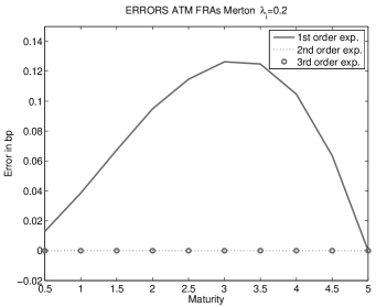
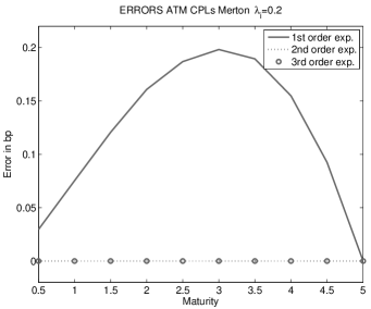
Figure 5.1. Drift expansion: low volatility scenario.

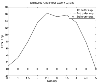
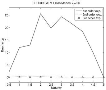
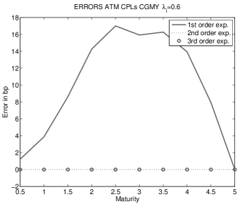
Figure 5.2. Drift expansion: high volatility scenario.

Furthermore, we notice that for low volatility even the first order expansion can be considered adequate, since the maximum of the absolute error is smaller than 0.2 bp. Conversely, for the high volatility case, the second order expansion is necessary to get proper accuracy. However, going to the third order expansion or beyond appears to be unnecessary as there is no visible gain in accuracy ($<10^{-5}$ bp). Hence, in the next sections we will use the second order drift expansion as our benchmark case since any resulting error is small enough to be disregarded.

In Table 5.1, CPU times are shown when simulating 10000 paths on an Intel i7 PC running Matlab. Here we can see that highly significant speed-up is achieved when truncating the higher order drift terms, whereas the decrease in speed when taking higher order approximations into account is relatively negligible. The CGMY is slower than the Merton model due to the much higher jump intensity needed in its approximation. We conjecture that the efficiency can be improved using the methods of [KHT10], but this lies outside the focus of this article.

	Full Drift	1st order	2nd order	3rd order
Merton	358.5	3.95	4.48	4.79
CGMY	471.9	16.29	16.59	16.74

Table 5.1. CPU Times (secs) for 10000 paths

Finally, to conclude the subsection we should also mention that pricing errors for swaptions and ratchet caplets(not shown here) are of similar order of magnitude as in case of caplets.

5.2. Performance of the log-Lévy approximations

Next we study the performance of the log-Lévy approximations. We increase the number of rates to the more realistic setting of $N=20$ and consider the pricing of FRAs, caplets, sticky ratchet caplets and swaptions. We consider swaptions on swap rates over the periods $(T_{i},T_{i}+3)$ years. Since we have established that errors from the drift expansion can be disregarded, we consider as the benchmark case the second order drift expansion studied in the previous section. In Figures 5.3 and 5.4 we plot prices from the frozen drift, the first and second order log-Lévy approximations of section 3, and include the annuity approximation of the following section for completeness (for the path-independent derivatives). We use both the Merton and the CGMY model. We can observe that the frozen drift is consistently beaten by both the 1st and 2nd order approximation in both models and for all four products. The 1st and 2nd order log-Lévy approximations have a quite similar performance suggesting that second order approximation may not be necessary. Note that other parameter values (higher/lower intensity for Merton and fatter tails/slower tail decay for CGMY) have also been studied and again the results are qualitatively the same.

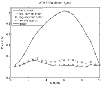
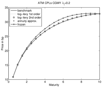
Figure 5.3. Prices for the Merton and CGMY models.

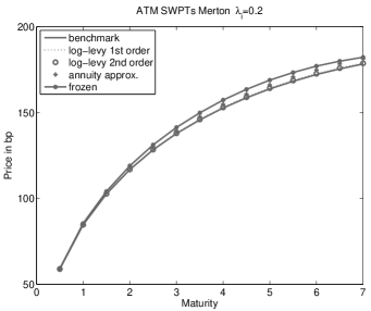
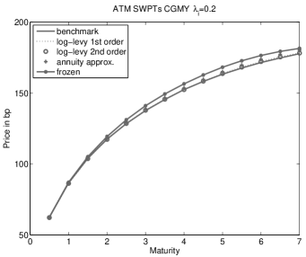
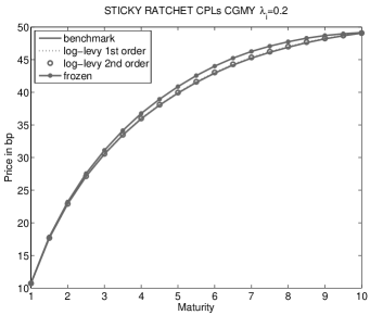
Figure 5.4. Prices for the Merton and CGMY models.

Concluding, the log-Lévy approximations offer an alternative to the Euler (or predictor-corrector) discretization of the actual dynamics which can be simulated faster and yields almost as accurate options prices.

6. Approximation of annuities

In the lognormal LIBOR market model, it is well documented that problems may occur for high volatilities due to a proportionally large Monte Carlo variance in the annuity term used for discounting under the terminal measure, see [Bev10] and [GBM06]. Motivated by this numerical problem, we will derive an approximation of the annuity term in the spirit of [GBM06, §10.13].

Let us define the annuity term

$$A_{i}(t)=\prod_{j=i+1}^{N}(1+\delta_{j}L_{j}(t)),$$ (6.1)

and consider the vector of log-LIBOR rates $G=[G_{i+1},\dots,G_{N}]$. We define a function $f:\mathbb{R}^{N-i}\to\mathbb{R}$ such that

$$(x_{i+1},\dots,x_{N})=x\longmapsto\prod_{j=i+1}^{N}(1+\delta_{j}\mathrm{e}^{x_{j}}).$$

The partial derivatives of $f$ are provided by

$$f_{k}(x)=\frac{\partial}{\partial x_{k}}f(x)=\prod_{\begin{subarray}{c}j=i+1\\ j\neq k\end{subarray}}^{N}(1+\delta_{j}\mathrm{e}^{x_{j}})\delta_{k}\mathrm{e}^{x_{k}}=f(x)\frac{\delta_{k}\mathrm{e}^{x_{k}}}{1+\delta_{k}\mathrm{e}^{x_{k}}},$$

for all $i+1\leq k\leq N$, while we obviously have that

$$f(G(t))=A_{i}(t).$$ (6.2)

Applying Itô’s formula to $f(G)$, we have that

$$f(G(t))=A_{i}(t) =A_{i}(0)+\sum_{j=i+1}^{N}\int_{0}^{t}f_{j}(G(s-))\mathrm{d}G_{j}(s)$$

$$\quad+\frac{1}{2}\sum_{j,k=i+1}^{N}\int_{0}^{t}f_{j,k}(G(s-))\mathrm{d}\langle G_{k},G_{j}(s)\rangle^{c}(s)$$

$$\quad+\sum_{s\leq t}\left\{\Delta f(G(s))-\sum_{j=i+1}^{N}f_{j}(G(s-))\Delta G_{j}(s)\right\}.$$ (6.3)

Noting that the annuity is a $\mathrm{I\kern-1.99997ptP}_{*}$-martingale, we will focus on the martingale parts of (6) in the sequel. Using (3.1) and the fact that $H$ is also a $\mathrm{I\kern-1.99997ptP}_{*}$-martingale, we get that the martingale part of the first summand is

$$\sum_{j=i+1}^{N}\int_{0}^{t}f_{j}(G(s-))\lambda_{j}(s)\mathrm{d}H(s) =\sum_{j=i+1}^{N}\int_{0}^{t}\frac{\delta_{j}L_{j}(s-)}{1+\delta_{j}L_{j}(s-)}f(G(s-))\lambda_{j}(s)\mathrm{d}H(s)$$

$$=\int_{0}^{t}A_{i}(s-)\sum_{j=i+1}^{N}\frac{\delta_{j}L_{j}(s-)}{1+\delta_{j}L_{j}(s-)}\lambda_{j}(s)\mathrm{d}H(s).$$

The second summand is omitted, while the final summands yields that

$$\sum_{s\leq t}\left\{\Delta f(G(s))-\sum_{j=i+1}^{N}f_{j}(G(s-))\Delta G_{j}(s)\right\}$$

$$=\sum_{s\leq t}\left\{\Delta A_{i}(s)-A_{i}(s-)\sum_{j=i+1}^{N}\frac{\delta_{j}L_{j}(s-)}{1+\delta_{j}L_{j}(s-)}\Delta G_{j}(s)\right\}$$

$$=\sum_{s\leq t}\left\{\Delta A_{i}(s)-A_{i}(s-)\sum_{j=i+1}^{N}\frac{\delta_{j}L_{j}(s-)}{1+\delta_{j}L_{j}(s-)}\lambda_{j}(s)\Delta H(s)\right\}$$

$$=\int_{0}^{t}\int_{\mathbb{R}^{m}}\left\{A_{i}(s)-A_{i}(s-)-A_{i}(s-)\sum_{j=i+1}^{N}\frac{\delta_{j}L_{j}(s-)}{1+\delta_{j}L_{j}(s-)}\lambda_{j}(s)x\right\}\widetilde{\mu}(\mathrm{d}s,\mathrm{d}x)$$

$$\,\,-\int_{0}^{t}\int_{\mathbb{R}^{m}}\left\{A_{i}(s)-A_{i}(s-)-A_{i}(s-)\sum_{j=i+1}^{N}\frac{\delta_{j}L_{j}(s-)}{1+\delta_{j}L_{j}(s-)}\lambda_{j}(s)x\right\}F(s,\mathrm{d}x)\mathrm{d}s,$$ (6.4)

where the quantity $A_{i}(s)$ in the last two integrals should be understood as

$$A_{i}(s)=\prod_{j=i+1}^{N}\left(1+\delta_{j}\exp\big{\{}G_{j}(s-)+\lambda_{j}^{\mathsf{T}}(s)x\big{\}}\right).$$ (6.5)

Collecting all the pieces together, we have that the annuity $A_{i}$ satisfies the following integrated SDE

$$A_{i}(t) =A_{i}(0)+\int_{0}^{t}A_{i}(s-)\Lambda_{i}(s-)\mathrm{d}H(s)$$

$$\quad+\int_{0}^{t}\int_{\mathbb{R}^{m}}\left\{A_{i}(s)-A_{i}(s-)-A_{i}(s-)\Lambda_{i}(s-)\right\}\widetilde{\mu}(\mathrm{d}s,\mathrm{d}x)$$

or, equivalently

$$A_{i}(t) =A_{i}(0)+\int_{0}^{t}A_{i}(s-)\Lambda_{i}(s-)\mathrm{d}H(s)$$

$$\quad+\int_{0}^{t}\int_{\mathbb{R}^{m}}A_{i}(s-)\left\{\frac{A_{i}(s)}{A_{i}(s-)}-1-\Lambda_{i}(s-)x\right\}\widetilde{\mu}(\mathrm{d}s,\mathrm{d}x),$$ (6.6)

where

$$\Lambda_{i}(s-)=\sum_{j=i+1}^{N}\frac{\delta_{j}L_{j}(s-)}{1+\delta_{j}L_{j}(s-)}\lambda_{j}(s).$$ (6.7)

The solution of the SDE (6) is the stochastic exponential, thus we get that

$$A_{i}(t) =A_{i}(0)\exp\left(\int_{0}^{t}\Lambda_{i}(s-)\mathrm{d}W(s)-\frac{1}{2}\int_{0}^{t}\Lambda_{i}^{\mathsf{T}}\Lambda_{i}(s-)\mathrm{d}s\right.$$

$$\qquad\qquad\qquad+\int_{0}^{t}\int_{\mathbb{R}^{m}}\left\{\frac{A_{i}(s)}{A_{i}(s-)}-1\right\}\widetilde{\mu}(\mathrm{d}s,\mathrm{d}x)$$ (6.8)

$$\qquad\qquad\qquad\left.-\int_{0}^{t}\int_{\mathbb{R}^{m}}\left(\log\left\{\frac{A_{i}(s)}{A_{i}(s-)}\right\}-\frac{A_{i}(s)}{A_{i}(s-)}+1\right)\mu(\mathrm{d}s,\mathrm{d}x)\right),$$

where again $A_{i}(s)$ should be understood as in (6.5). By freezing the random terms in the drifts and jump sizes in the above dynamics we get an alternative approximation for the annuity term. Note that the resulting approximation is also a log-Lévy approximation.

We can now use this approximation to price caplets and swaptions, noting that their respective payoffs can be written in terms of annuities:

$$\mathbb{C}_{0} =B_{N+1}(0)\,\mathrm{I\kern-1.99997ptE}_{\mathrm{I\kern-1.39998ptP}_{*}}\left[\frac{A_{i}(T_{i+1})}{A_{i}(T_{i})}\Big{(}A_{i-1}(T_{i})-\left(1+\delta_{i}K\right)A_{i}(T_{i})\Big{)}^{+}\right],$$ (6.9)

$$\mathbb{S}_{0} =B_{N+1}(0)\,\mathrm{I\kern-1.99997ptE}_{\mathrm{I\kern-1.39998ptP}_{*}}\left[\left(-\sum^{m}_{k=i}c_{k}A_{k-1}(T_{i})\right)^{+}\right],$$ (6.10)

where the $c_{k}$’s are defined in (5.9). A similar expression can be derived for the sticky ratchet caplet.

6.1. Performance of the annuity approximation

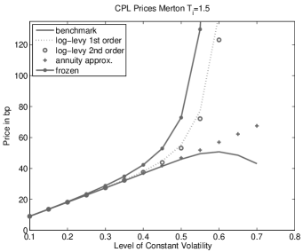
Figure 6.1. Caplet prices as a function of volatility ($N=20$).

In Figure 6.1, the quality of the various approximations is studied for a number of at-the-money caplets as a function of the volatility. As before we set the number of rates to $N=20$, and simulate 50000 paths for each volatility level. The plot is for the Merton model while the results are similar for CGMY. Using that at-the-money call option prices are increasing and roughly linear functions of volatility (see for example [Wil98], [BS94] and [BFW04] for the case of non-Gaussian distributions), we can observe that only the annuity approximation produces sensible option prices at all levels of volatility. Moreover, even the benchmark case fails when volatility grows beyond $30\%$, meaning that the Monte Carlo simulation has failed to converge. The frozen drift fails at even lower levels of volatility, while the log-Lévy approximations fail at a higher level, similar to the benchmark case. The annuity approximation works for all (higher) levels and also, as we have seen in Figures 5.3 and 5.4, for the low levels. One should therefore be careful when the average (across maturity) at-the-money implied volatilities are above 30% which is indeed the case in the current market for USD denominated LIBOR caplets where volatilities range from roughly 80% in the short end to 25% in the long end (source: Bloomberg).

Moreover, in Figure 6.2 we observe that this problem becomes significantly less severe when limiting the number of rates to 10 with $\delta_{i}=1$ instead of 20 with $\delta_{i}=0.5$. Needless to say, limiting the number of rates is rarely a possibility in practice.

Figure 6.2. Caplet prices as a function of volatility ($N=10$).

In order to intuitively understand why this approximation performs better in the high volatility case than the other methods (e.g. the standard Euler scheme or the log-Lévy approximations), let us just concentrate on the lognormal case. We have from (6) that

$$\log A_{i}(t)\cong\sum_{j=i+1}^{N}\frac{\delta_{j}L_{j}(0)}{1+\delta_{j}L_{j}(0)}\lambda_{j}\cdot\sqrt{t}\,\mathcal{N}+\text{deterministic terms},$$ (6.11)

where $\mathcal{N}$ denotes a standard normal random variate. On the other hand, from (6.1), we get that

$$\log A_{i}(t)\cong\sum_{j=i+1}^{N}\delta_{j}\exp\left(\lambda_{j}\cdot\sqrt{t}\,\mathcal{N}+\text{random terms}\right),$$ (6.12)

where actually the method of approximation will only affect the random terms. We can easily conclude from (6.11) and (6.12) that the variance of the annuity approximation is significantly lower that the variance of the standard representation, which results in the faster convergence of the Monte Carlo method. Thus, the annuity log-Lévy approximation should be interpreted as a variance reduction technique for the LIBOR market model.

7. Economically meaningful multi-dimensional Lévy measures via subordination

Next, we reflect on the properties the driving process should have for practical applications and provide some recommendations. In an economically realistic Lévy LIBOR model the very structure of the Lévy measure is important. Since, from an economic point of view, any jump in the daily rate typically affects all segments of the yield curve, we require in our modeling that, at a jump time, all the LIBORs jump, not only the first or second half of the LIBOR curve for example. Moreover, this requirement should be fulfilled regardless of the structure of the loading factors $\lambda_{i}$; the latter may be inferred from some calibration procedure for instance. A natural way to meet this property is to take Lévy measures which are absolutely continuous. In a jump-diffusion setting this can be easily established by taking as Lévy measure the product of one dimensional absolutely continuous probability measures $p_{i}$, i.e.

$$\nu(\mathrm{d}x)=p_{1}(\mathrm{d}x_{1})\cdot\cdot\cdot p_{m}(\mathrm{d}x_{m});$$ (7.1)

see [BS11]. In this paper we consider LIBOR models based on Lévy processes with possibly infinite activity, thus having available flexible and realistic LIBOR models possibly without Wiener part (i.e. $\alpha\equiv 0$). However, Lévy measures of infinite activity cannot be obtained by simply taking the product of a set of one-dimensional Lévy measures of infinite activity. Nonetheless, we seek for absolutely continuous infinite activity Lévy measures such that the entailed jump processes maintain certain (weak) independence properties. Such measures may be constructed by Brownian subordination (see e.g. [CT04]) as outlined below.

Let $W$ be a Wiener process on $\mathbb{R}^{m}$. The characteristic function of $W(t)$ is given by

$$\mathrm{I\kern-1.99997ptE}\left[\mathrm{e}^{izW(t)}\right]=\mathrm{e}^{-\frac{t}{2}\left\|z\right\|^{2}}=:\mathrm{e}^{t\Psi(z)},\quad z\in\mathbb{R}^{m}.$$

We now consider a subordinator $(S_{t})_{t\geq 0}$ on $\mathbb{R}_{+},$ with Lévy triplet $(0,0,\rho),$ and with Laplace exponent $\Xi$, i.e.

$$\mathrm{I\kern-1.99997ptE}\left[\mathrm{e}^{uS_{t}}\right]=\mathrm{e}^{t\Xi(u)}:=\exp\Big{(}t\int_{\left(0,\infty\right)}\left(\mathrm{e}^{su}-1\right)\rho(\mathrm{d}s)\Big{)},\quad u\leq 0.$$

Then the $m$-dimensional process $Y$ defined by

$$Y(t):=W(S_{t})$$

has characteristic function

$$\mathrm{I\kern-1.99997ptE}\left[\mathrm{e}^{iz^{\mathsf{T}}Y(t)}\right] =\mathrm{I\kern-1.99997ptE}\left[\mathrm{I\kern-1.99997ptE}\left[\mathrm{e}^{iz^{\mathsf{T}}W(S_{t})}|S_{t}\right]\right]=\mathrm{I\kern-1.99997ptE}\left[\mathrm{e}^{S_{t}\Psi(z)}\right]=\mathrm{e}^{t\Xi(\Psi(z))}$$

$$=\exp\left[t\int_{\left(0,\infty\right)}\left(\mathrm{e}^{s\Psi(z)}-1\right)\rho(\mathrm{d}s)\right]$$

$$=\exp\left[t\int_{\left(0,\infty\right)}\left(\mathrm{e}^{-\frac{s}{2}\left\|z\right\|^{2}}-1\right)\rho(\mathrm{d}s)\right]=:\exp\left[t\Phi(z)\right]$$

As a result, $Y$ is a pure jump martingale Lévy process with Lévy measure $\nu^{Y}$ satisfying

$$\Phi(z)=\int_{\left(0,\infty\right)}\left(\mathrm{e}^{-\frac{s}{2}\left\|z\right\|^{2}}-1\right)\rho(\mathrm{d}s)=\int_{\mathbb{R}^{m}}(\mathrm{e}^{\mathfrak{i}z^{\mathsf{T}}x}-1-\mathfrak{i}z^{\mathsf{T}}x)\nu^{Y}(\mathrm{d}x).$$ (7.2)

It is easily checked that

$$\nu^{Y}(\mathrm{d}x)=\int_{0}^{\infty}\frac{1}{\left(\sqrt{2\pi s}\right)^{m}}\mathrm{e}^{-\frac{1}{2s}||x||^{2}}\rho(\mathrm{d}s)\mathrm{d}x,$$ (7.3)

which is a measure with absolutely continuous support.

Example 7.1.

Let $(S_{t})_{t\geq 0}$ be the inverse Gaussian subordinator with

$$\rho(\mathrm{d}s)=\frac{c\mathrm{e}^{-\lambda s}}{s^{3/2}}1_{\{s>0\}}\mathrm{d}s,\quad\text{ and }\quad\mathrm{I\kern-1.99997ptE}\left[\mathrm{e}^{uS_{t}}\right]=\mathrm{e}^{-2ct\sqrt{\pi}\left(\sqrt{\lambda-u}-\sqrt{\lambda}\right)}.$$

Then, (7.2) is known explicitly as

$$\Phi(z)=-2c\sqrt{\pi}\left(\sqrt{\lambda+\frac{\sigma^{2}}{2}\left\|z\right\|^{2}}-\sqrt{\lambda}\right),$$

e.g. see [CT04].

Example 7.2.

Let $(S_{t})_{t\geq 0}$ be a Lévy subordinator with the following properties:

$$\rho(\mathrm{d}t) =C\mathrm{e}^{-\frac{t}{4}G}D_{-Y}(G)1_{\{t>0\}}\mathrm{d}t,$$

$$\Xi(u) =2C\Gamma(-Y)\left[(G^{2}-2u)^{Y/2}\cos\left(Y\arctan\left(\frac{\sqrt{-2u}}{G}\right)\right)-G^{Y}\right],$$

where $D$ is the parabolic cylinder function. Then, (7.2) is known explicitly as the Lévy exponent of the CGMY process, cf. (5), with $G=M$; see [MY08].

Remark 7.3.

By taking in (2.2) $F(s,\mathrm{d}x):=\nu^{Y}(\mathrm{d}x)$ with $\nu^{Y}$ given by (7.3), the jump-part of (2.2) is represented by the process $Y$ constructed above. It is easy to see that $Y$ has uncorrelated components, although they are generally not independent. Indeed, $Y(t)$ has mean zero and we have that

$$\mathrm{I\kern-1.99997ptE}\left[Y^{(k)}(t)Y^{(l)}(t)\right]=\mathrm{I\kern-1.99997ptE}\left[\mathrm{I\kern-1.99997ptE}\left[W^{(k)}(S_{t})W^{(l)}(S_{t})\mid S_{t}\right]\right]=0,\quad 1\leq k<l\leq m.$$

Thus in contrast to the jump-diffusion situation in [BS11] where all components jump at the same time independently, here the components of $Y$ still jump at the same time but in an uncorrelated rather than in an independent way.

8. Concluding summary

We have presented a tractable numerical approach to simulate trajectories of a general Lévy LIBOR model in an efficient way. By this method we construct efficient approximations to the computationally demanding drift term in the Lévy LIBOR dynamics. We have shown that, due to these these approximations, we arrive at a significantly more accurate log-Lévy approximation than the one obtained by the usual “frozen drift” approximation. The performance of the method is illustrated by several examples. The presentation is embedded in a flexibly structured multi-factor Lévy LIBOR model which allows for natural modeling of mutual LIBOR dependences (via incorporating suitable correlation structures). As such the paper supports practical implementations of Lévy interest rate models that, until now, played mostly an academic role.

Appendix A Computation of the drift

A.1. Full expansion in terms of cumulants

We will derive a representation for the integral term of the drift (2.7) which does not involve an integration over random terms. Let us denote the integral term by

$$\mathbb{B}_{i}:=\int_{\mathbb{R}^{m}}\left(\left(\mathrm{e}^{\lambda_{i}^{\mathsf{T}}x}-1\right){\displaystyle\prod\limits_{j=i+1}^{N}}\left(1+\frac{\delta_{j}L_{j-}\left(\mathrm{e}^{\lambda_{i}^{\mathsf{T}}x}-1\right)}{1+\delta_{j}L_{j-}}\right)-\lambda_{i}^{\mathsf{T}}x\right)F(\cdot,\mathrm{d}x).$$

Observe that

$$\prod\limits_{j=1}^{l}\left(1+w_{j}\right) =1+\sum_{1\leq j\leq l}w_{j}+\sum_{1\leq j_{1}<j_{2}\leq l}w_{j_{1}}w_{j_{2}}$$

$$\quad+\sum_{1\leq j_{1}<j_{2}<j_{3}\leq l}w_{j_{1}}w_{j_{2}}w_{j_{3}}+...+\,w_{1}\cdots w_{l}$$

$$=1+\sum_{p=1}^{l}S_{p}^{l}(w_{1},...,w_{l}),$$

where $S_{p}^{l}$ denotes the elementary symmetric polynomial of degree $p$ in $l$ variables, i.e.

$$S_{p}^{l}(w_{1},...,w_{l}):=\sum_{1\leq j_{1}<\cdot\cdot\cdot<j_{p}\leq l}w_{j_{1}}\cdots w_{j_{p}},\text{ \ \ }1\leq p\leq l.$$

Thus $\mathbb{B}_{i}$ may be rearranged as follows:

$$\mathbb{B}_{i} =\int\left(\mathrm{e}^{\lambda_{i}^{\mathsf{T}}x}-1-\lambda_{i}^{\mathsf{T}}x\right)F(\cdot,\mathrm{d}x)+\sum_{p=1}^{N-i}\int\left(\mathrm{e}^{\lambda_{i}^{\mathsf{T}}x}-1\right)\,\times$$

$$\qquad\quad S_{p}^{N-i}\left(\frac{\delta_{i+1}L_{i+1-}\left(\mathrm{e}^{\lambda_{i+1}^{\mathsf{T}}x}-1\right)}{1+\delta_{i+1}L_{i+1-}},\dots,\frac{\delta_{N}L_{N-}\left(\mathrm{e}^{\lambda_{N}^{\mathsf{T}}x}-1\right)}{1+\delta_{N}L_{N-}}\right)F(\cdot,\mathrm{d}x)$$

$$:=(I)+(II).$$

Let us consider in $(II)$ for $p\geq 1$ the term

$$\!\!\int\!\!\left(\mathrm{e}^{\lambda_{i}^{\mathsf{T}}x}-1\right)\!\!S_{p}^{N-i}\!\!\left(\!\!\frac{\delta_{i+1}L_{i+1-}\left(\mathrm{e}^{\lambda_{i+1}^{\mathsf{T}}x}\!-1\right)}{1+\delta_{i+1}L_{i+1-}},\ldots,\frac{\delta_{N}L_{N-}\left(\mathrm{e}^{\lambda_{N}^{\mathsf{T}}x}-1\right)}{1+\delta_{N}L_{N-}}\!\!\right)F(\cdot,\mathrm{d}x)$$

$$=\sum_{i<j_{1}<\cdots<j_{p}\leq N}\frac{\delta_{j_{1}}L_{j_{1}-}}{1+\delta_{j_{1}}L_{j_{1}-}}\cdots\frac{\delta_{j_{p}}L_{j_{p}-}}{1+\delta_{j_{p}}L_{j_{p}-}}$$

$$\qquad\qquad\times\int\left(\mathrm{e}^{\lambda_{i}^{\mathsf{T}}x}-1\right)\left(\mathrm{e}^{\lambda_{j_{1}}^{\mathsf{T}}x}-1\right)\cdots\left(\mathrm{e}^{\lambda_{j_{p}}^{\mathsf{T}}x}-1\right)F(\cdot,\mathrm{d}x).$$

With $j_{0}:=i,$ we may write

$$\left(\mathrm{e}^{\lambda_{i}^{\mathsf{T}}x}-1\right)\left(\mathrm{e}^{\lambda_{j_{1}}^{\mathsf{T}}x}-1\right)\cdots\left(\mathrm{e}^{\lambda_{j_{p}}^{\mathsf{T}}x}-1\right)$$ (A.1)

$$=(-1)^{p+1}\left(1-\mathrm{e}^{\lambda_{j_{0}}^{\mathsf{T}}x}\right)\left(1-\mathrm{e}^{\lambda_{j_{1}}^{\mathsf{T}}x}\right)\cdots\left(1-\mathrm{e}^{\lambda_{j_{p}}^{\mathsf{T}}x}\right)$$

$$=(-1)^{p+1}\left[1+\sum_{q=1}^{p+1}S_{q}^{p+1}(-\mathrm{e}^{\lambda_{j_{0}}^{\mathsf{T}}x},\dots,-\mathrm{e}^{\lambda_{j_{p}}^{\mathsf{T}}x})\right]=(-1)^{p+1}\left[1+(\ast)\right]$$

where

$$(\ast) =\sum_{q=1}^{p+1}(-1)^{q}S_{q}^{p+1}(\mathrm{e}^{\lambda_{j_{0}}^{\mathsf{T}}x},\dots,\mathrm{e}^{\lambda_{j_{p}}^{\mathsf{T}}x})=\sum_{q=1}^{p+1}(-1)^{q}\!\!\sum_{0\leq r_{1}<\cdots<r_{q}\leq p}\!\!\mathrm{e}^{\lambda_{j_{r_{1}}}^{\mathsf{T}}x}\cdots\mathrm{e}^{\lambda_{j_{r_{q}}}^{\mathsf{T}}x}$$

$$=\sum_{q=1}^{p+1}(-1)^{q}\sum_{0\leq r_{1}<\cdots<r_{q}\leq p}\text{ }\underset{O(\left\|x\right\|^{2})}{\underbrace{\left(\mathrm{e}^{\lambda_{j_{r_{1}}}^{\mathsf{T}}x+\cdots+\lambda_{j_{r_{q}}}^{\mathsf{T}}x}-1-(\lambda_{j_{r_{1}}}^{\mathsf{T}}x+\cdots+\lambda_{j_{r_{q}}}^{\mathsf{T}}x)\right)}}$$

$$\quad+\sum_{q=1}^{p+1}(-1)^{q}\sum_{0\leq r_{1}<\cdots<r_{q}\leq p}\left(1+\lambda_{j_{r_{1}}}^{\mathsf{T}}x+\cdots+\lambda_{j_{r_{q}}}^{\mathsf{T}}x\right).$$

Obviously, expression (A.1) is of order $O(\left\|x\right\|^{2})$ for any $p\geq 1$, hence (!) it must hold

$$1+\sum_{q=1}^{p+1}(-1)^{q}\sum_{0\leq r_{1}<\cdots<r_{q}\leq p}\left(1+\lambda_{j_{r_{1}}}^{\mathsf{T}}x+\cdots+\lambda_{j_{r_{q}}}^{\mathsf{T}}x\right)=0.$$

Therefore, we can deduce the following representation for the integral term

$$\mathbb{B}_{i} =\int\left(\mathrm{e}^{\lambda_{i}^{\mathsf{T}}x}-1-\lambda_{i}^{\mathsf{T}}x\right)F(\cdot,\mathrm{d}x)$$

$$\quad+\sum_{p=1}^{N-i}\sum_{i<j_{1}<\cdots<j_{p}\leq N}\frac{\delta_{j_{1}}L_{j_{1}-}}{1+\delta_{j_{1}}L_{j_{1}-}}\cdots\frac{\delta_{j_{p}}L_{j_{p}-}}{1+\delta_{j_{p}}L_{j_{p}-}}\sum_{q=1}^{p+1}(-1)^{p+q+1}$$

$$\times\!\sum_{0\leq r_{1}<\cdots<r_{q}\leq p}\int\!\left(\mathrm{e}^{\left(\lambda_{j_{r_{1}}}+\cdots+\lambda_{j_{r_{q}}}\right)^{\mathsf{T}}x}-1-\left(\lambda_{j_{r_{1}}}+\cdots+\lambda_{j_{r_{q}}}\right)^{\mathsf{T}}\!x\right)F(\cdot,\mathrm{d}x)$$

$$=\widehat{\kappa}(\lambda_{i})+\sum_{p=1}^{N-i}\sum_{i<j_{1}<\cdots<j_{p}\leq N}\frac{\delta_{j_{1}}L_{j_{1}-}}{1+\delta_{j_{1}}L_{j_{1}-}}\cdots\frac{\delta_{j_{p}}L_{j_{p}-}}{1+\delta_{j_{p}}L_{j_{p}-}}$$

$$\qquad\qquad\quad\times\sum_{q=1}^{p+1}(-1)^{p+q+1}\sum_{0\leq r_{1}<\cdots<r_{q}\leq p}\widehat{\kappa}\left(\lambda_{j_{r_{1}}}+\cdots+\lambda_{j_{r_{q}}}\right).$$ (A.2)

A.2. First order expansion of (A.1)

Let us consider the first order expansion of $\mathbb{B}_{i}$; we get

$$\mathbb{B}_{i} =\widehat{\kappa}(\lambda_{i})+\sum_{i<j<n}\frac{\delta_{j}L_{j-}}{1+\delta_{j}L_{j-}}\sum_{q=1}^{2}(-1)^{q}\sum_{0\leq r_{1}<\cdots<r_{q}\leq 1}\widehat{\kappa}\left(\lambda_{j_{r_{1}}}+\cdots+\lambda_{j_{r_{q}}}\right)$$

$$\quad+O(\left\|L\right\|^{2}).$$

Note that

$$\sum_{q=1}^{2}(-1)^{q}\sum_{0\leq r_{1}<\cdots<r_{q}\leq 1}\widehat{\kappa}\left(\lambda_{j_{r_{1}}}+\cdots+\lambda_{j_{r_{q}}}\right)$$

$$\quad=-\sum_{0\leq r_{1}\leq 1}\text{}\widehat{\kappa}\left(\lambda_{j_{r_{1}}}\right)\,\,+\sum_{0\leq r_{1}<r_{2}\leq 1}\widehat{\kappa}\left(\lambda_{j_{r_{1}}}+\lambda_{j_{r_{2}}}\right)$$

$$\quad=-\widehat{\kappa}\left(\lambda_{j_{0}}\right)-\widehat{\kappa}\left(\lambda_{j_{1}}\right)+\widehat{\kappa}\left(\lambda_{j_{0}}+\lambda_{j_{1}}\right).$$

Thus we obtain the following expression for the first order expansion of the integral term $\mathbb{B}_{i}$

$$\mathbb{B}_{i}^{\prime} =\widehat{\kappa}(\lambda_{i})+\sum_{i<j\leq N}\frac{\delta_{j}L_{j-}}{1+\delta_{j}L_{j-}}\big{(}\widehat{\kappa}(\lambda_{i}+\lambda_{j})-\widehat{\kappa}(\lambda_{i})-\widehat{\kappa}(\lambda_{j})\big{)},$$ (A.3)

which leads to the following approximation for the drift term $b_{i}$ in (2.7)

$$b_{i}^{\prime} =\kappa(\lambda_{i})+\sum_{i<j\leq N}\frac{\delta_{j}L_{j-}}{1+\delta_{j}L_{j-}}\big{(}\kappa(\lambda_{i}+\lambda_{j})-\kappa(\lambda_{i})-\kappa(\lambda_{j})\big{)},$$ (A.4)

taking also the terms stemming from the diffusion into account.

A.3. Second order expansion of (A.1)

Analogously, we can also derive a second order expansion of $\mathbb{B}_{i}$; we get

$$\mathbb{B}_{i} =\widehat{\kappa}(\lambda_{i})+\sum_{i<j\leq N}\frac{\delta_{j}L_{j-}}{1+\delta_{j}L_{j-}}\big{(}\widehat{\kappa}(\lambda_{i}+\lambda_{j})-\widehat{\kappa}(\lambda_{i})-\widehat{\kappa}(\lambda_{j})\big{)}$$

$$\quad+\sum_{i+1\leq k<l\leq N}\frac{\delta_{k}L_{k-}}{1+\delta_{k}L_{k-}}\frac{\delta_{l}L_{l-}}{1+\delta_{l}L_{l-}}\Big{(}\widehat{\kappa}(\lambda_{i}+\lambda_{k}+\lambda_{l})-\widehat{\kappa}(\lambda_{i}+\lambda_{k})$$

$$\qquad\qquad\qquad-\widehat{\kappa}(\lambda_{i}+\lambda_{l})-\widehat{\kappa}(\lambda_{k}+\lambda_{l})+\widehat{\kappa}(\lambda_{i})+\widehat{\kappa}(\lambda_{k})+\widehat{\kappa}(\lambda_{l})\Big{)}$$

$$\quad+O(\left\|L\right\|^{3}),$$

which leads to the following second order expansion of $b_{i}$ in (2.7)

$$b_{i}^{\prime\prime} =\kappa(\lambda_{i})+\sum_{i<j\leq N}\frac{\delta_{j}L_{j-}}{1+\delta_{j}L_{j-}}\big{(}\kappa(\lambda_{i}+\lambda_{j})-\kappa(\lambda_{i})-\kappa(\lambda_{j})\big{)}$$

$$\quad+\sum_{i+1\leq k<l\leq N}\frac{\delta_{k}L_{k-}}{1+\delta_{k}L_{k-}}\frac{\delta_{l}L_{l-}}{1+\delta_{l}L_{l-}}\Big{(}\widehat{\kappa}(\lambda_{i}+\lambda_{k}+\lambda_{l})-\widehat{\kappa}(\lambda_{i}+\lambda_{k})$$

$$\qquad\qquad-\widehat{\kappa}(\lambda_{i}+\lambda_{l})-\widehat{\kappa}(\lambda_{k}+\lambda_{l})+\widehat{\kappa}(\lambda_{i})+\widehat{\kappa}(\lambda_{k})+\widehat{\kappa}(\lambda_{l})\Big{)}.$$ (A.5)

Appendix B Derivation of (3.12)

Using the Itô formula for general semimartingales (cf. [JS03, Theorem I.4.57]) we have

$$Z_{j} =Z_{j}(0)+\int_{0}^{\cdot}f^{\prime}(G_{j}(s-))\mathrm{d}G_{j}+\frac{1}{2}\int_{0}^{\cdot}f^{\prime\prime}(G_{j})\mathrm{d}\langle G_{j}^{c},G_{j}^{c}\rangle$$

$$\quad+\sum_{0<s\leq\cdot}\left(f(G_{j}(s))-f\left(G_{j}(s-)\right)-f^{\prime}\left(G_{j}(s-)\right)\Delta G_{j}(s)\right),$$ (B.1)

where $\langle G_{j}^{c},G_{j}^{c}\rangle$ denotes the quadratic variation of the continuous martingale part of $G_{j},$ that is

$$\mathrm{d}\langle G_{j}^{c},G_{j}^{c}\rangle(s)=\left|\lambda_{j}\right|^{2}(s)\alpha(s)\mathrm{d}s.$$ (B.2)

The sum in (B), using (3.1), may be written as

$$\sum_{0<s\leq\cdot}\left(f(G_{j}(s-)+\Delta G_{j}(s))-f\left(G_{j}(s-)\right)-f^{\prime}\left(G_{j}(s-)\right)\Delta G_{j}(s)\right)$$ (B.3)

$$=\int_{0}^{\cdot}\int_{\mathbb{R}^{m}}\left(f(G_{j}(s-)+\lambda_{j}^{\mathsf{T}}x)-f\left(G_{j}(s-)\right)-f^{\prime}\left(G_{j}(s-)\right)\lambda_{j}^{\mathsf{T}}x\right)\mu(\mathrm{d}s,\mathrm{d}x)$$

$$=\int_{0}^{\cdot}\int_{\mathbb{R}^{m}}\left(f(G_{j}(s-)+\lambda_{j}^{\mathsf{T}}x)-f\left(G_{j}(s-)\right)-f^{\prime}\left(G_{j}(s-)\right)\lambda_{j}^{\mathsf{T}}x\right)F(s,\mathrm{d}x)\mathrm{d}s$$

$$\,\,\,+\int_{0}^{\cdot}\int_{\mathbb{R}^{m}}\left(f(G_{j}(s-)+\lambda_{j}^{\mathsf{T}}x)-f\left(G_{j}(s-)\right)-f^{\prime}\left(G_{j}(s-)\right)\lambda_{j}^{\mathsf{T}}x\right)\widetilde{\mu}(\mathrm{d}s,\mathrm{d}x).$$

Moreover,

$$\int_{0}^{\cdot}f^{\prime}(G_{j}(s-))\mathrm{d}G_{j} =\int_{0}^{\cdot}f^{\prime}(G_{j}(s-))b_{j}\mathrm{d}s+\int_{0}^{t}f^{\prime}(G_{j}(s-))\sqrt{\alpha}\lambda_{j}^{\mathsf{T}}\mathrm{d}W$$

$$\quad+\int_{0}^{\cdot}\int_{\mathbb{R}^{m}}f^{\prime}(G_{j}(s-))\lambda_{j}^{\mathsf{T}}x\,\widetilde{\mu}(\mathrm{d}s,\mathrm{d}x).$$ (B.4)

Finally, by plugging (B.2), (B.3) and (B) into (B), (3.12) follows.

Appendix C Derivation of (3.14)

The computations are completely analogous to Appendix B, thus omitted for brevity. The coefficients of $Y_{kl}$ in (3.14) are

$$A_{kl}(s,L(s)) =\sum_{i=k,l}g_{i}(G_{k}(s-),G_{l}(s-))b_{i}(s)$$

$$\qquad+\frac{1}{2}\sum_{i,j=k,l}\int_{0}^{\cdot}g_{ij}(G_{k}(s-),G_{l}(s-))\lambda_{i}(s)\lambda_{j}(s)\alpha(s)$$

$$+\int_{\mathbb{R}^{m}}\bigg{(}g(G_{k}(s-)+\lambda_{k}^{\mathsf{T}}x,G_{l}(s-)+\lambda_{l}^{\mathsf{T}}x)-g(G_{k}(s),G_{l}(s))$$

$$\qquad\qquad-\sum_{i=k,l}g_{i}(G_{k}(s-),G_{l}(s-))\lambda_{i}^{\mathsf{T}}x\bigg{)}F(s,\mathrm{d}x),$$ (C.1)

$$B_{kl}^{\mathsf{T}}(s,L_{kl}(s)) =\sum_{i=k,l}g_{i}(G_{k}(s-),G_{l}(s-))\sqrt{\alpha(s)}\lambda_{i}^{\mathsf{T}}(s)$$ (C.2)

and

$$C_{kl}(s,L_{kl}(s),x) =\sum_{i=k,l}g_{i}(G_{k}(s-),G_{l}(s-))\lambda_{i}^{\mathsf{T}}(s)x$$

$$\quad+g\big{(}G_{k}(s-)+\lambda_{k}^{\mathsf{T}}x,G_{l}(s-)+\lambda_{l}^{\mathsf{T}}x\big{)}-g\big{(}G_{k}(s),G_{l}(s)\big{)}$$

$$\qquad-\sum_{i=k,l}g_{i}(G_{k}(s-),G_{l}(s-))\lambda_{i}^{\mathsf{T}}x.$$ (C.3)

Here $L_{kl}(s):=(L_{k}(s),L_{l}(s))$ and denotes that $B_{kl}$ and $C_{kl}$ depend on $L_{k}$ and $L_{l}$ (via $G_{k}$ and $G_{l}$).

References

- [ABR05] L. Andersen and R. Brotherton-Ratcliffe. Extended LIBOR market models with stochastic volatility. J. Comput. Finance, 9:1–40, 2005.
- [AG07] S. Asmussen and P. W. Glynn. Stochastic Simulation: Algorithms and Analysis. Springer, 2007.
- [BDB01] A. Brace, T. Dun, and G. Barton. Towards a central interest rate model. In E. Jouini, J. Cvitanić, and M. Musiela, editors, Option Pricing, Interest Rates and Risk Management, pages 278–313. Cambridge University Press, 2001.
- [BEJP11] M. Beinhofer, E. Eberlein, A. Janssen, and M. Polley. Correlations in Lévy interest rate models. Quant. Finance, 11:1315–1327, 2011.
- [Bev10] C. Beveridge. Very long-stepping in the spot measure of the LIBOR market model. Wilmott J., 2(6):289–299, 2010.
- [BFW04] D. Backus, S. Foresi, and L. Wu. Accounting for biases in Black-Scholes. SSRN/585623, 2004.
- [BGM97] A. Brace, D. Ga̧tarek, and M. Musiela. The market model of interest rate dynamics. Math. Finance, 7:127–155, 1997.
- [Bla76] F. Black. The pricing of commodity contracts. J. Financ. Econ., 3:167–179, 1976.
- [BMS09] D. Belomestny, S. Mathew, and J. Schoenmakers. Multiple stochastic volatility extension of the LIBOR market model and its implementation. Monte Carlo Methods Appl., 15:285–310, 2009.
- [BS94] M. Brenner and M.G. Subrahmanyam. A simple approach to option valuation and hedging in the Black-Scholes model. Financial Analysts J., 50(2):25–28, 1994.
- [BS11] D. Belomestny and J. Schoenmakers. A jump-diffusion LIBOR model and its robust calibration. Quant. Finance, 11:529–546, 2011.
- [CGMY02] P. Carr, H. Geman, D. B. Madan, and M. Yor. The fine structure of asset returns: An empirical investigation. J. Business, 75:305–332, 2002.
- [CT04] R. Cont and P. Tankov. Financial Modelling with Jump Processes. Chapman and Hall/CRC Press, 2004.
- [DBS01] T. Dun, G. Barton, and E. Schlögl. Simulated swaption delta-hedging in the lognormal forward LIBOR model. Int. J. Theor. Appl. Finance, 4:677–709, 2001.
- [DG05] A. Daniluk and D. Ga̧tarek. A fully log-normal LIBOR market model. Risk, 18(9):115–118, 2005.
- [EK07] E. Eberlein and W. Kluge. Calibration of Lévy term structure models. In M. Fu, R. A. Jarrow, J.-Y. Yen, and R. J. Elliott, editors, Advances in Mathematical Finance: In Honor of Dilip B. Madan, pages 155–180. Birkhäuser, 2007.
- [EÖ05] E. Eberlein and F. Özkan. The Lévy LIBOR model. Finance Stoch., 9:327–348, 2005.
- [GBM06] D. Gatarek, P. Bachert, and R. Maksymiuk. The LIBOR Market Model in Practice. Wiley, 2006.
- [GK03] P. Glasserman and S. G. Kou. The term structure of simple forward rates with jump risk. Math. Finance, 13:383–410, 2003.
- [GM03a] P. Glasserman and N. Merener. Cap and swaption approximations in LIBOR market models with jumps. J. Comput. Finance, 7:1–36, 2003.
- [GM03b] P. Glasserman and N. Merener. Numerical solution of jump-diffusion LIBOR market models. Finance Stoch., 7:1–27, 2003.
- [GZ00] P. Glasserman and X. Zhao. Arbitrage-free discretization of lognormal forward LIBOR and swap rate models. Finance Stoch., 4:35–68, 2000.
- [HJJ01] C. Hunter, P. Jäckel, and M. Joshi. Getting the drift. Risk, 14:81–84, 2001.
- [Jam97] F. Jamshidian. LIBOR and swap market models and measures. Finance Stoch., 1:293–330, 1997.
- [Jam99] F. Jamshidian. LIBOR market model with semimartingales. Working Paper, NetAnalytic Ltd., 1999.
- [JS03] J. Jacod and A. N. Shiryaev. Limit Theorems for Stochastic Processes. Springer, 2nd edition, 2003.
- [JS08] M. Joshi and A. Stacey. New and robust drift approximations for the LIBOR market model. Quant. Finance, 8:427–434, 2008.
- [KHT10] A. Kohatsu-Higa and P. Tankov. Jump-adapted discretization schemes for Lévy-driven SDEs. Stochastic Process. Appl., 120:2258–2285, 2010.
- [Klu05] W. Kluge. Time-inhomogeneous Lévy processes in interest rate and credit risk models. PhD thesis, Univ. Freiburg, 2005.
- [KSS02] O. Kurbanmuradov, K. Sabelfeld, and J. Schoenmakers. Lognormal approximations to LIBOR market models. J. Comput. Finance, 6:69–100, 2002.
- [MSS97] K. R. Miltersen, K. Sandmann, and D. Sondermann. Closed form solutions for term structure derivatives with log-normal interest rates. J. Finance, 52:409–430, 1997.
- [MY08] D. B. Madan and M. Yor. Representing the CGMY and Meixner processes as time changed Brownian motions. J. Comput. Finance, 12:27–47, 2008.
- [PS10] A. Papapantoleon and D. Skovmand. Picard approximation of stochastic differential equations and application to LIBOR models. Preprint, arXiv/1007:3362, 2010.
- [PT06] J. Poirot and P. Tankov. Monte Carlo option pricing for tempered stable (CGMY) processes. Asia-Pac. Finan. Markets, 13:327–344, 2006.
- [Ros01] J. Rosiński. Series representations of Lévy processes from the perspective of point processes. In O. E. Barndorff-Nielsen, Th. Mikosch, and S. I. Resnick, editors, Lévy Processes: Theory and Applications, pages 401–415. Birkhäuser, 2001.
- [Sch02] E. Schlögl. A multicurrency extension of the lognormal interest rate market models. Finance Stoch., 6:173–196, 2002.
- [Sch05] J. Schoenmakers. Robust LIBOR Modelling and Pricing of Derivative Products. Chapman & Hall/CRC Press, 2005.
- [Wil98] P. Wilmott. Derivatives: The Theory and Practice of Financial Engineering. Wiley, 1998.
- [WZ06] L. Wu and F. Zhang. LIBOR market model with stochastic volatility. J. Industr. Manag. Optim., 2:199–227, 2006.