Ice-Creams and Wedge Graphs

Abstract

What is the minimum angle $\alpha>0$ such that given any set of $\alpha$-directional antennas (that is, antennas each of which can communicate along a wedge of angle $\alpha$), one can always assign a direction to each antenna such that the resulting communication graph is connected? Here two antennas are connected by an edge if and only if each lies in the wedge assigned to the other. This problem was recently presented by Carmi, Katz, Lotker, and Rosén [2] who also found the minimum such $\alpha$ namely $\alpha=\frac{\pi}{3}$. In this paper we give a simple proof of this result. Moreover, we obtain a much stronger and optimal result (see Theorem 1) saying in particular that one can chose the directions of the antennas so that the communication graph has diameter $\leq 4$.

Our main tool is a surprisingly basic geometric lemma that is of independent interest. We show that for every compact convex set $S$ in the plane and every $0<\alpha<\pi$, there exist a point $O$ and two supporting lines to $S$ passing through $O$ and touching $S$ at two single points $X$ and $Y$, respectively, such that $|OX|=|OY|$ and the angle between the two lines is $\alpha$.

1 Antennas, Wedges, and Ice-Creams

Imagine the following situation. You are a manufacturer of antennas. In order to save power, your antennas should communicate along a wedge-shape area, that is, an angular and practically infinite section of certain angle $\alpha$ whose apex is the antenna. The smaller the angle is the better it is in terms of power saving. You are supposed to build many copies of these antennas to be used in various different communication networks. You know nothing about the future positioning of the antennas and you want them to be generic in the sense that they will fit to any possible finite set of locations. When installed, each antenna may be directed to an arbitrary direction that

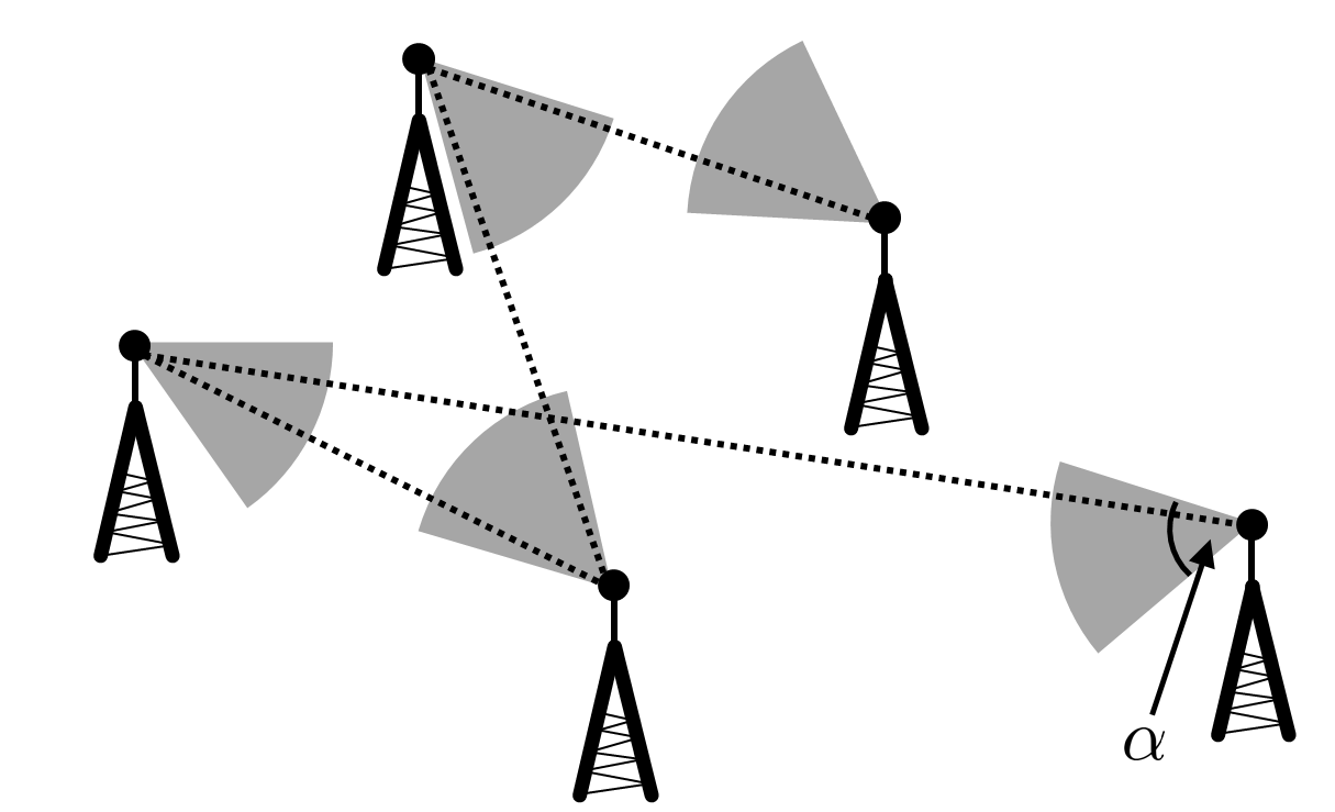
Figure 1: a set of $\alpha$-directional antennas and their (connected) communication graph.

will stay fixed forever. Therefore, you wish to find the minimum $\alpha>0$ so that no matter what finite set $P$ of locations of the antennas is given, one can always install the antennas and direct them so that they can communicate with each other. This is to say that the communication graph of the antennas should be a connected graph. The communication graph is the graph whose vertex set is the set $P$ and two vertices (antennas) are connected by an edge if the corresponding two antennas can directly communicate with each other, that is, each is within the transmission-reception wedge of the other (see Figure 1 for an illustration).

This problem was formulated by Carmi, Katz, Lotker, and Rosén [2], who also found the optimal $\alpha$ which is $\alpha=\frac{\pi}{3}$ (a different model of a directed communication graph of directional antennas of bounded transmission range was studied in [1, 3, 4]).

In this paper we provide a much simpler and more elegant proof of this result. We also improve on the result in [2] by obtaining a much simpler connected communication graph for $\alpha=\frac{\pi}{3}$ whose diameter is at most $4$. Our graph in fact consists of a path of length $2$ while every other vertex is connected by an edge to one of the three vertices of the path.

In order to state our result and bring the proof we now formalize some of the notions above.

Given two rays $q$ and $r$ with a common apex in the plane, we denote by $wedge({q,r})$ the closed convex part of the plane bounded by $q$ and $r$. For three noncollinear points in the plane $A,B,C$ we denote by $\angle ABC$ the wedge $wedge({\overrightarrow{BA},\overrightarrow{BC}})$, whose apex is the point $B$. $\angle ABC$ is a wedge of angle $\measuredangle ABC$.

Let $W_{1},\ldots,W_{n}$ be $n$ wedges with pairwise distinct apexes. The wedge-graph of $W_{1},\ldots,W_{n}$ is by definition the graph whose vertices correspond to the apexes $p_{1},\ldots,p_{n}$ of $W_{1},\ldots,W_{n}$, respectively, where two apexes $p_{i}$ and $p_{j}$ are joined by an edge iff $p_{i}\in W_{j}$ and $p_{j}\in W_{i}$.

Using this terminology we wish to prove the following theorem whose first part was proved by Carmi et al. [2].

Theorem 1.

Let $P$ be a set of $n$ points in general position in the plane and let $h$ be the number of vertices of the convex hull of $P$. One can always find in $O(n\log h)$-time $n$ wedges of angle $\frac{\pi}{3}$ whose apexes are the $n$ points of $P$ such that the wedge-graph with respect to these wedges is connected. Moreover, we can find wedges so that the wedge graph consists of a path of length $2$ and each of the other vertices in the graph is connected by an edge to one of the three vertices of the path.

The angle $\frac{\pi}{3}$ in Theorem 1 is best possible, as shown in [2]. Indeed, for any $\alpha<\frac{\pi}{3}$ one cannot create a connected communication graph for a set of $\alpha$-directional antennas that are located at the vertices of an equilateral triangle and on one of its edges.

We note that the result in Theorem 1 is optimal in the sense that it is not always possible to find an assignment of wedges to the points so that the wedge graph consists of less than three vertices the union of neighbors of which is the entire set of vertices of the graph. To see this consider a set of points evenly distributed on a circle. Notice that if each wedge is of angle $\alpha\leq\frac{\pi}{3}$, then in any wedge graph each vertex is a neighbor of at most one third of the vertices.

Our main tool in proving Theorem 1 is a basic geometric lemma that we call the “Ice-Cream Lemma”. Suppose that we put one scoop of ice-cream in a very large 2-dimensional cone, such that the ice-cream touches each side of the cone at a single point. The distances from these points to the apex of the cone are not necessarily equal. However, we show that there is always a way of putting the ice-cream in the cone such that they are equal. More formally, we prove:

Lemma 1 (Ice-cream Lemma).

Let $S$ be a compact convex set in the plane and fix $0<\alpha<\pi$. There exist a point $O$ in the plane and two rays, $q$ and $r$, emanating from $O$ and touching $S$ at two single points $X$ and $Y$, respectively, that satisfy $|OX|=|OY|$ and the angle bounded by $p$ and $q$ is $\alpha$.

See Figure 2 for an illustration.

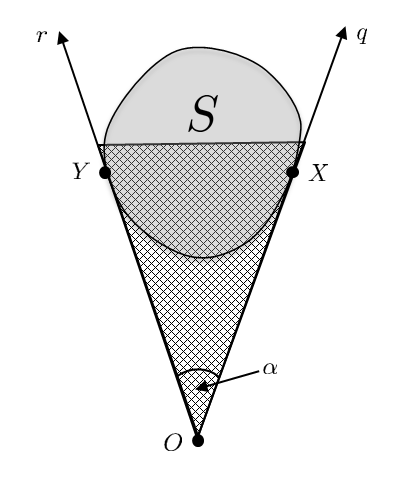
Figure 2: An illustration of the Ice-cream Lemma

The requirement in Lemma 1 that the two rays touch $S$ at single points will be crucial in our proof of Theorem 1.

At a first glance the statement in Lemma 1 probably looks very intuitive and it may seem that it should follow directly from a simple mean-value-theorem argument. However, this is not quite the case. Although the proof (we will give two different proofs) indeed uses a continuity argument it is not the most trivial one. The reader is encouraged to spend few minutes trying to come up with a simple argument just to get the feeling of Lemma 1 before continuing further.

Because the proof of Lemma 1 is completely independent of Theorem 1 and of its proof, we first show, in the next section, how to prove Theorem 1 using Lemma 1. We postpone the two proofs of the Ice-Cream Lemma to the last section.

2 Proof of Theorem 1 using Lemma 1

Let $P$ be a set of $n$ points in general position in the plane. We denote the convex hull of $P$ by $\mathcal{CH}\left(P\right)$, and recall that it can be computed in $O(n\log h)$ time [5]. Call two vertices of $\mathcal{CH}\left(P\right)$ a good pair if there are a point $O$ and two rays $q,r$ emanating from it creating an angle of $\frac{\pi}{3}$ such that $X\in q,Y\in r$, $|OX|=|OY|$, and $\mathcal{CH}\left(P\right)\subset\angle XOY$. Note that given $\mathcal{CH}\left(P\right)$ and two vertices of it $X,Y$, we can check in constant time whether $X,Y$ is a good pair. Indeed there are exactly two points that form an equilateral triangle with $X,Y$, and for each of these two possible locations of $O$, we only need to check whether the neighbors of $X$ and $Y$ in $\mathcal{CH}\left(P\right)$ lie in $\angle XOY$.

Lemma 1 guarantees that $\mathcal{CH}\left(P\right)$ has a good pair. Next we describe an efficient way to find such a good pair. Suppose that $X,Y$ is a good pair. Observe that there are two other rays that form an angle of measure $\pi/3$, contain $\mathcal{CH}\left(P\right)$ in their wedge, and such that one of them contains an edge of $\mathcal{CH}\left(P\right)$ that is adjacent to $X$ or $Y$ and the other ray contains the other point. (These rays can be obtained by continuously rotating the ray through $X$ while forcing the ray through $Y$ to form a $\pi/3$ angle with it, until an edge of $\mathcal{CH}\left(P\right)$ is hit. Note that the distances from $X$ and $Y$ to the apex of the new wedge are no longer equal.) Therefore, to find a good pair $X,Y$, it is enough to find for every edge $(X,X^{\prime})$ of $\mathcal{CH}\left(P\right)$ the (at most four) points $Y$ such that $Y$ is a vertex of $\mathcal{CH}\left(P\right)$ and a line through $Y$ that forms $\pi/3$ angle with the line through $(X,X^{\prime})$ supports $\mathcal{CH}\left(P\right)$. For every such point, we can check in constant time whether $X,Y$ or $X^{\prime},Y$ is a good pair. Finding the points $Y$ for an edge $(X,X^{\prime})$ as above can be done in $O(\log h)$-time by a binary search on the vertices of $\mathcal{CH}\left(P\right)$. Thus, a good pair $(X,Y)$ and the corresponding $r$, $q$, and $O$ can be found in $O(n\log h)$-time.

Let $\ell$ be a line creating an angle of $\frac{\pi}{3}$ with both $q$ and $r$ such that $P$ is contained in the region bounded by $q,r,$ and $\ell$ and there is a point $Z\in P$ on $\ell$. (Note that $Z$ can be found in $O(\log h)$-time.) Let $A,B$ denote the intersection points of $\ell$ with $q$ and $r$, respectively (see Figure 3).

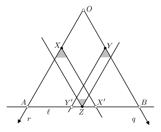
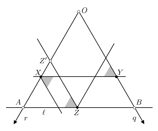
Figure 3: Proof of Theorem 1.

Let $X^{\prime}\in\ell$ be such that $\Delta AXX^{\prime}$ is equilateral. Let $Y^{\prime}\in\ell$ be such that $\Delta BYY^{\prime}$ is equilateral.

Case 1: $Z\in\angle AXX^{\prime}$ and $Z\in\angle BYY^{\prime}$. In this case $\measuredangle XZY\leq\frac{\pi}{3}$. Let $W_{Z}$ be a wedge of angle $\frac{\pi}{3}$ with apex $Z$ containing both $X$ and $Y$. Let $W_{X}$ be the wedge $\angle AXX^{\prime}$ and let $W_{Y}$ be the wedge $\angle BYY^{\prime}$. See Figure 3. Observe that the wedge-graph that corresponds to $W_{X},W_{Y},W_{Z}$ is connected ($Z$ is connected by edges to both $X$ and $Y$).

Case 2: Without loss of generality $Z\notin\angle AXX^{\prime}$. In this case let $W_{Y}=\angle OYX$, let $W_{X}=\angle YXX^{\prime}$, and let $W_{Z}=\angle AZZ^{\prime}$, where $Z^{\prime}\in OA$ is such that $\Delta AZZ^{\prime}$ is equilateral. See Figure 3. Again we have that $X$ is connected by edges to both $Y$ and $Z$ in the wedge-graph that corresponds to $W_{X},W_{Y},W_{Z}$.

Finally, observe that in both cases the wedge-graph contains a 2-path on the vertices $X,Y,Z$, and $W_{X}\cup W_{Y}\cup W_{Z}$ contains $\Delta OAB$ and hence the entire set of points $P$. We can now easily find for each point $D\in P\setminus\{X,Y,Z\}$ in constant time a wedge of angle $\frac{\pi}{3}$ and apex $D$ such that in the wedge-graph that corresponds to the set of all these edges, each such $D$ will be connected to one of $X,Y,Z$.  

It is left to prove our main tool, Lemma 1. This is done in the next section.

3 Two proofs of the “Ice-cream Lemma”

We will give two different proofs for Lemma 1.

Proof I. In this proof we will assume that the set $S$ is strictly convex, that is, we assume that the boundary of $S$ does not contain a straight line segment. We assume this in order to simplify the proof, however this assumption is not critical and can be avoided. We bring this proof mainly for its independent interest (see Claim 1 below). The second proof of Lemma 1 is shorter and applies for general $S$.

For an angle $0\leq\theta\leq 2\pi$ we denote by $S_{\theta}$ a (possibly translated) copy of $S$ rotated in an angle of $\theta$. Let $q$ and $r$ be two rays emanating from the origin $O$ and creating an angle $\alpha$. Observe that for every $\theta$ there exists a unique translation of $S_{\theta}$ that is contained in $wedge({q,r})$ and both $q$ and $r$ touch $S_{\theta}$ at a single point (here we use the fact that $S$ is strictly convex). For every $0\leq\theta\leq 2\pi$ we denote by $X(\theta)$ and $Y(\theta)$ the two touching points on $q$ and on $r$, respectively. Let $f(\theta)$ denote the distance between $Y(\theta)$ and the origin (see Figure 4).

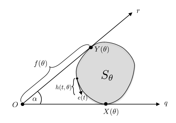
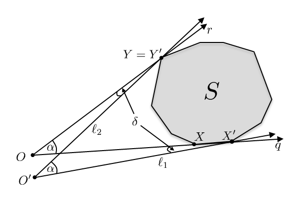
Figure 4: Illustrations for the proofs of the Ice-cream Lemma

Claim 1.

$\int_{0}^{2\pi}f\,\mathrm{d}\theta={\cal P}(S)\frac{1+\cos\alpha}{\sin\alpha}$, where ${\cal P}(S)$ denotes the perimeter of the set $S$.

Proof. Without loss of generality assume that the ray $q$ coincides with the positive part of the $x$-axis and $r$ lies in the upper half-plane.

Consider the boundary $\partial S$ with the positive (counterclockwise) orientation. Note that since $S$ is convex, at each point $p\in\partial S$ there is a unique supporting line pointing forward (here after positive tangent), and a unique supporting line pointing backwards (the two tangent lines coincide iff $\partial S$ is smooth at $p$). Let $e:[0,{\cal P}(S))\to\partial S$ be a unit speed curve traveling around $\partial S$. We define a function $h(t,\theta)$ in the following way: If $e(t)$ belongs to the part of the boundary of $S_{\theta}$ between $X(\theta)$ and $Y(\theta)$ that is visible from $O$, then we set $h(t,\theta)$ to be equal to the length of the orthogonal projection of the unit positive tangent at $e(t)$ on the $y$-axis (see Figure 4). Otherwise we set $h(t,\theta)=0$.

The simple but important observation here is that for every $0\leq\theta\leq 2\pi$ the expression $\int_{0}^{{\cal P}(S)}h(t,\theta)\,\mathrm{d}t$ is equal to the $y$-coordinate of $Y(\theta)$. This, in turn, is equal by definition to $f(\theta)\sin\alpha$. To see this observation take a small portion of the boundary of $S(\theta)$ of length $\mathrm{d}t$ that is visible from $O$. Its orthogonal projection on the $y$-axis has (by definition) length $h(t,\theta)\mathrm{d}t$. Notice that the orthogonal projection of the entire part of the boundary of $S(\theta)$ that is visible from $O$ on the $y$-axis (whose length, therefore, equals to this integral) is precisely all the points on the $y$-axis with smaller $y$-coordinate than that of $Y(\theta)$.

By Fubini’s theorem we have:

$$\int_{0}^{2\pi}f(\theta)\sin\alpha\,\mathrm{d}\theta=\int_{0}^{2\pi}\int_{0}^{{\cal P}(S)}h(t,\theta)\,\mathrm{d}t\,\mathrm{d}\theta=\int_{o}^{{\cal P}(S)}\int_{0}^{2\pi}h(t,\theta)\,\mathrm{d}\theta\,\mathrm{d}t$$ (1)

Moreover, for every $t$ we have:

$$\int_{0}^{2\pi}h(t,\theta)\,\mathrm{d}\theta=\int_{\pi+\alpha}^{2\pi}|\sin(\theta)|\,\mathrm{d}\theta=(1+\cos\alpha).$$ (2)

To see this observe that $e(t)$ is visible from $O$ through the rotation of $S$ precisely from where it lies on the ray $r$ until it lies on the ray $q$. Through this period the angle which the positive tangent at $e(t)$ creates with the $x$-axis varies from $\pi+\alpha$ to $2\pi$.

Combining (1) and (2) we conclude:

$$\int_{0}^{2\pi}f(\theta)\sin\alpha\,\mathrm{d}\theta = \int_{0}^{{\cal P}(S)}\int_{0}^{2\pi}h(e,\theta)\,\mathrm{d}\theta\,\mathrm{d}t=$$

$$= \int_{0}^{{\cal P}(S)}(1+\cos\alpha)\,\mathrm{d}t={\cal P}(S)(1+\cos\alpha),$$

which in turn implies the desired result: $\int_{0}^{2\pi}f(\theta)\,\mathrm{d}\theta={\cal P}(S)\frac{1+\cos\alpha}{\sin\alpha}$.

 

Analogously to $f(\theta)$ we define $g(\theta)$ to be the distance from $X(\theta)$ to the origin $O$. Lemma 1 is equivalent to saying that there is a $\theta$ for which $f(\theta)=g(\theta)$. By a similar argument or by applying the result of Claim 1 to a reflection of $S$, we deduce that $\int_{0}^{2\pi}g(\theta)\,\mathrm{d}\theta={\cal P}(S)\frac{1+\cos\alpha}{\sin\alpha}$. In particular $\int_{0}^{2\pi}f(\theta)\,\mathrm{d}\theta=\int_{0}^{2\pi}g(\theta)\,\mathrm{d}\theta$. Because $f$ and $g$ are continuous we may now conclude the following:

Corollary 1.

Assume that $S$ is strictly convex, then there exists $\theta$ between $0$ and $2\pi$ such that $f(\theta)=g(\theta)$.

This completes the proof of Lemma 1 in the case where $S$ is strictly convex.  

We now bring the second proof of Lemma 1. This proof is shorter than the first one and does not rely on the strict convexity assumption.

Proof II. Consider the point $O$ such that the two tangents of $S$ through $O$ create an angle of $\alpha$ and such that the area of the convex hull of $\{O\}\cup S$ is maximum. By a simple compactness argument such $O$ exists.

We will show that the point $O$ satisfies the requirements of the lemma. Let $q$ and $r$ be the two rays emanating from $O$ and tangent to $S$. Let $X$ and $X^{\prime}$ be the end points of the (possibly degenerate) line segment $q\cap S$ and assume $|OX|\leq|OX^{\prime}|$. Similarly, let $Y$ and $Y^{\prime}$ be the two (possible equal) points such that the intersection of $r$ and $S$ is the line segment connecting $Y$ and $Y^{\prime}$ and assume $|OY|\leq|OY^{\prime}|$.

We claim that $|OX^{\prime}|\leq|OY|$ (and similarly $|OY^{\prime}|\leq|OX|$). This will imply immediately the desired result because in this case $|OX|\leq|OX^{\prime}|\leq|OY|\leq|OY^{\prime}|\leq|OX|$ from which we conclude that $X=X^{\prime}$, $Y=Y^{\prime}$, and $|OX|=|OY|$.

Assume to the contrary that $|OX^{\prime}|>|OY|$. Without loss of generality assume that $S$ lies to the left of $q$ and to the right of $r$ (see Figure 4). Let $\delta>0$ be very small positive number and let $\ell_{1}$ be the directed line supporting $S$ having $S$ to its left that is obtained from $\overline{OX^{\prime}}$ by rotating it counterclockwise at angle $\delta$. Let $\ell_{2}$ be the directed line supporting $S$ having $S$ to its right that is obtained from $\overline{OY}$ by rotating it counterclockwise at angle $\delta$ (see Figure 4).

Let $O^{\prime}$ be the intersection point of $\ell_{1}$ and $\ell_{2}$. Note that $\ell_{1}$ and $\ell_{2}$ create an angle of $\alpha$. We claim that the area of the convex hull of $\{O^{\prime}\}\cup S$ is greater than the area of the convex hull of $\{O\}\cup S$. Indeed, up to lower order terms the difference between the two equals $\frac{1}{2}(|OX^{\prime}|^{2}-|OY|^{2})\sin(\delta)>0$. This contradicts the choice of the point $O$.  

Remarks.

Lemma 1 clearly holds for non-convex (but compact) sets $S$ as well, since we can apply it on the convex hull of $S$ and observe that if a line supports the convex hull and intersects it in a single point, then this point must belong to $S$.

From both proofs of Lemma 1 it follows, and is rather intuitive as well, that one can always find at least two points $O$ that satisfy the requirements of the lemma. In the first proof notice that both functions $f$ and $g$ are periodic and therefore if they have the same integral over $[0,2\pi]$, they must agree in at least two distinct points, as they are continuous. In the second proof one can choose a point $O$ that minimizes the area of the convex hull of $O$ and $S$ and obtain a different solution.

Department of Mathematics, Physics, and Computer Science, University of Haifa at Oranim, Tivon 36006, Israel. ackerman@sci.haifa.ac.il

Mathematics Department, Hebrew University of Jerusalem, Jerusalem, Israel. gelander@math.huji.ac.il

Mathematics Department, Technion—Israel Institute of Technology, Haifa 32000, Israel. room@math.technion.ac.il

References

- [1] I. Caragiannis, C. Kaklamanis, E. Kranakis, D. Krizanc and A. Wiese, Communication in wireless networks with directional antennas, Proc. 20th Symp. on Parallelism in Algorithms and Architectures, 344–351, 2008.
- [2] P. Carmi, M.J. Katz, Z. Lotker, A. Rosén, Connectivity guarantees for wireless networks with directional antennas, Computational Geometry: Theory and Applications, to appear.
- [3] M. Damian and R.Y. Flatland, Spanning properties of graphs induced by directional antennas, Electronic Proc. 20th Fall Workshop on Computational Geometry, Stony Brook University, Stony Brook, NY, 2010.
- [4] S. Dobrev, E. Kranakis, D. Krizanc, J. Opatrny, O. Ponce, and L. Stacho, Strong connectivity in sensor networks with given number of directional antennae of bounded angle, Proc. 4th Int. Conf. on Combinatorial Optimization and Applications, 72–86, 2010.
- [5] D.G. Kirkpatrick and R. Seidel, The ultimate planar convex hull algorithm, SIAM J. on Computing, 15(1):287–299, 1986.