Synergy in spreading processes: from exploitative to explorative foraging strategies

Abstract

An epidemiological model which incorporates synergistic effects that allow the infectivity and/or susceptibility of hosts to be dependent on the number of infected neighbours is proposed. Constructive synergy induces an exploitative behaviour which results in a rapid invasion that infects a large number of hosts. Interfering synergy leads to a slower and sparser explorative foraging strategy that traverses larger distances by infecting fewer hosts. The model can be mapped to a dynamical bond-percolation with spatial correlations that affect the mechanism of spread but do not influence the critical behaviour of epidemics.

The identification of criteria to predict whether or not a spreading agent such as an infectious pathogen, rumour or opinion will invade a population is of great relevance both in biology and social sciences AndersonMay86:invasion ; Murray_02:book ; Castellano_RMP2009 ; Centola_Science2010 . Numerous models have been proposed to gauge the invasiveness of spreading agents and assess the effectiveness of control in preventing invasion of epidemics AndersonMay86:invasion ; Murray_02:book ; Castellano_RMP2009 ; Gubbins00:thresholds ; Keeling01:fmdsci ; Dodds_PRL2004 ; Shao_Havlin_Stanley_PRL2009 ; Maksim_NatPhys2010 ; Ben-Jacob_Nature1994 ; Ferreira_PRE2002 . Within the context of infectious diseases, much theoretical work has been done for well-mixed populations but invasion in stochastic, spatially-structured, individual-based models Keeling99:localinvasion ; Grassberger1983 ; Sander et al. (2002); PerezReche_JRSInterface2010 ; Kenah2007 ; Miller_PRE2007 closer to real epidemics Bailey00:perc ; Otten04:perc2 ; Davis_Nature2008 ; Pastor-Satorras_Book2004 has also been considered. These models do not deal with synergistic effects in transmission of infection thus assuming independent and identical action between hosts. This would suggest that multiple challenges to a susceptible host from one, two or more neighbouring infected hosts are independent and not influenced by the local environment. However, there is evidence for the existence of such effects in systems subject to colonisation by fungal and bacterial pathogens Rayner_Mycologia1991_review ; Ben-Jacob_Nature1994 , as well as in tumour growth Liotta_Nature2001 ; Ferreira_PRE2002 . Synergistic effects have also been experimentally reported in studies of opinion dynamics Castellano_RMP2009 , spread of behaviour Centola_Science2010 , and animal invasion Murray_02:book ; Gordon_Book2009 . The model presented in Ref. Dodds_PRL2004, incorporates some temporal synergistic effects but it deals with well-mixed populations and spatial synergistic effects are not considered. Models for opinion dynamics and animal invasion have considered some constructive synergistic spatial effects (e.g. population pressure Murray_02:book and social impact Castellano_RMP2009 ; Centola_PhysicaA2007 ). However, these effects are too simple to capture, for instance, possible changes in the foraging strategies of spreading agents that can significantly affect important features of invasions such as their size and time scales. Here, we present a model for spread of infection in spatially-structured populations and show that synergistic effects in transmission of infection have non-trivial and significant consequences on epidemics.

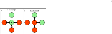
Figure 1: Mechanism for (a) r-synergy and (b) d-synergy. Dark (red online) and lighter (green online) circles correspond to infected and susceptible hosts, respectively. Arrows indicate possible events for transmission of infection. For r-synergy, the susceptibility of a recipient susceptible host ⓡ is enhanced (constructive synergy) or diminished (interfering synergy) in response to multiple simultaneous challenges from two or more neighbouring infected hosts (donors). The susceptibility of ⓡ depends on the number $n_{\text{r}}$ of neighbours simultaneously challenging it ($n_{\text{r}}=3$ in this example). For d-synergy, the infectivity of a donor host ⓓ depends upon the number $n_{\text{d}}$ of connections of this host to other infectious hosts that can share resources with the donor host. In this example, $n_{\text{d}}=1$ (connection indicated by an edge).

We consider an epidemic spreading through a population of susceptible hosts placed on the sites/nodes of a square lattice of size $L\times L$. The infection transmission rate between any donor-recipient (d-r) pair of hosts depends on the number of infected hosts in the neighbourhood of the d-r pair. We focus on two particular cases of the model denoted as r-synergy and d-synergy (Fig. 1).

The model is an extension of a basic spatial model for the SIR epidemic process in which hosts (sites) can be in one of the three states Grassberger1983 : susceptible (S), infected (I) or removed and fully immune to further infection (R). Once a host is infected, it stays in such a state for a fixed unit of time, $\tau=1$ and can pass infection during this infectious period to other S-neighbours, and then it is removed/recovered (I $\to$ R transition). The infection process (S $\to$ I transition) occurs through the pathogen being transmitted randomly with rate $\lambda_{\text{d-r}}(t)$ from one of the I-neighbours (donor) of the S-host (recipient). Synergistic effects make the rate $\lambda_{\text{d-r}}(t)$ dependent on the state of hosts in the neighbourhood of the particular d-r pair. By definition, $\lambda_{\text{d-r}}(t)$, is zero before the time of infection of the donor. Once the donor is infected, $\lambda_{\text{d-r}}(t)$ becomes positive but, in contrast to the basic SIR model Grassberger1983 ; Henkel_Hinrichsen_Book2009 , it can vary during the whole infectious period $\tau$ due to possible changes in the neighbourhood of the d-r pair. The transmission rate can be conveniently split into two contributions,

$$\lambda_{\text{d-r}}(t)=\max\{0,\alpha+\beta_{\text{d-r}}(t)\}~{},$$ (1)

where $\alpha\geq 0$ is the elementary rate of infection for an isolated d-r pair exhibiting no synergistic effects. It does not vary over the infectious period and is assumed to be the same for all d-r pairs. The rate $\beta_{\text{d-r}}(t)$ quantifies the degree of synergy present and is $\beta_{\text{d-r}}(t)=0$ in the absence of synergistic effects when the model reduces to the simple SIR process. The expression for $\beta_{\text{d-r}}(t)$ depends on the type of synergy. For r-synergy (Fig. 1(a)), we assume that $\beta_{\text{d-r}}(t)=\beta(n_{\text{r}}(t)-1)$, where $n_{\text{r}}(t)$ is the number of neighbours challenging a recipient host. The rate $\beta$ gives an effective measure of the strength of synergy which is constructive for $\beta>0$ and interfering if $\beta<0$. Such a form of $\beta_{\text{d-r}}(t)$ ensures that $\lambda_{\text{d-r}}=\alpha$ for non-synergistic transmissions with $n_{\text{r}}=1$. For d-synergy (Fig. 1(b)), we assume that $\beta_{\text{d-r}}(t)=\beta n_{\text{d}}(t)$, where $n_{\text{d}}(t)$ is the number of infected neighbours connected to a donor at time $t$ so that $\lambda_{\text{d-r}}=\alpha$ for an isolated infectious host with $n_{\text{d}}=0$.

Fig. 2 shows the phase diagram for epidemics starting from a single infected host placed in the centre of the lattice. The spread of infection has been numerically simulated by a continuous-time algorithm which is an extension of the n-fold way algorithm Fallert_PRE2008 . The threshold for invasion defines a line of critical points $\alpha_{\text{c}}(\beta)$ separating the non-invasive regime where the probability of invasion is $P_{\text{inv}}=0$ (in an infinite system) from the invasive regime characterised by $P_{\text{inv}}>0$ . The phase boundaries shown in Fig. 2 correspond to the values of $\alpha_{\text{c}}(\beta)$ for $L\to\infty$. The finite-size effects were accounted for and eliminated by means of finite-size scaling (see Appendices A and B).

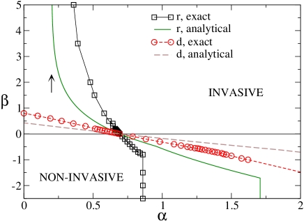
Figure 2: Phase diagram for synergistic epidemics. The exact phase boundaries are marked by squares for r-synergy and by circles for d-synergy. Epidemics are invasive if the parameters ($\alpha,\beta$) are on the right of the phase boundary. The arrow indicates the limiting value of $\alpha_{\text{c}}\simeq 0.2$ reached asymptotically by the phase boundary for r-synergy in the limit of large $\beta$ (not shown on the scale of the graph). The approximate phase boundaries obtained analytically by neglecting correlations in transmission of infection (cf. Appendix F) are shown for both r- (solid line) and d-synergy (dashed line).

For both types of synergy, $\alpha_{\text{c}}$ is a non-increasing function of $\beta$, as expected from the monotonic dependence of $\lambda_{\text{d-r}}$ on $\beta$ [Eq. (1)]. In the absence of synergy, the invasion thresholds for both types of synergy coincide with $\alpha_{\text{c}}(\beta=0)=\tau^{-1}\ln 2$ (cf. Fig. 2 and Appendix A). The larger deviations of $\alpha_{\text{c}}(\beta)$ from $\alpha_{\text{c}}(0)$ for a given $\beta$ observed for d-synergy are due to the fact that, except for the initially infected host, d-synergy is present in every transmission event with $\beta\neq 0$ because $n_{\text{d}}\geq 1$ for at least some time. In contrast, for r-synergy to be operative in a transmission event, there must be $n_{\text{r}}\geq 2$ attacking neighbours which is not necessarily the case in every transmission event.

For r-synergy with large positive values of $\beta$, the critical line $\alpha_{\text{c}}(\beta)$ tends towards the limiting value $\alpha_{\text{c}}(\infty)\simeq 0.2$ (Fig. 2). In this situation, $\lambda_{\text{d-r}}=\alpha<\infty$ for $n_{\text{r}}=1$ but $\lambda_{\text{d-r}}=\infty$ if $n_{\text{r}}>1$, meaning that hosts being simultaneously attacked by more than one neighbour are infected immediately. In cases with large interference in transmission (i.e. very negative $\beta$), the invasion threshold is located at $\alpha_{\text{c}}=0.86\pm 0.01$ independently of the value of $\beta$. In this regime, $\lambda_{\text{d-r}}$ does not depend on $\beta$ and corresponds to the limiting situation with $\lambda_{\text{d-r}}=\alpha$ for $n_{\text{r}}=1$ and $\lambda_{\text{d-r}}=0$ for any $n_{\text{r}}>1$.

For d-synergy and values of $\beta\gtrsim 0.8$, invasion is possible for any positive $\alpha$. The condition $\alpha>0$ is necessary in order for the epidemic to start from a single inoculated site. Once the pathogen is transmitted to one of the neighbours of the initially inoculated host, $n_{\text{d}}=1$ for the newly infected host. The combination of $n_{\text{d}}=1$ and synergy is sufficient to make invasion possible, irrespective of the value of $\alpha$.

Systems with constructive synergy are characterised by dense patterns of invasion (Fig. 3(a)). In contrast, the invaded region is more sparse for interfering synergy (Fig. 3(b)). This scenario applies to both d- and r-synergy. Despite the fact that patterns for interfering synergy are more sparse, it is striking that epidemics with interfering synergy can nevertheless be as invasive as epidemics with constructive synergy in terms of the spatial extent of infection. For instance, all the patterns shown in Fig. 3 have the same probability of invasion, $P_{\text{inv}}=0.5$. In terms of the mean spatial density of invasion defined as the relative number of hosts infected by the pathogen before invasion occurs with a given probability, we conclude that the larger the interference in transmission of the pathogen, the less damaging the invasion is (Appendix C). This result can be qualitatively understood as follows. Interfering synergy favours transmission of infection to hosts with few infected neighbours and disfavours transmission to hosts with several previously infected neighbours. Therefore, infection has a tendency to evolve towards poorly infected regions rather than infecting as many hosts as possible. These mechanisms are qualitatively similar for both types of synergy but the density of infection is larger for d-synergy than for r-synergy for any $\beta\neq 0$ (see Appendix C for more detail).

For constructive synergy, the patterns of invasion are not very much influenced by the particular type of synergy. For interfering synergy, the degree of branching of the paths followed by the pathogen is clearly smaller for d-synergy than for r-synergy (cf. panels in Fig. 3(b)). Branching is always possible for r-synergy. In contrast, the patterns of invasion for d-synergy display a branching transition for a value of $\alpha=\alpha_{\text{b}}(\beta)=-\beta$: branching occurs for $\alpha>\alpha_{\text{b}}(\beta)$ but it is absent for $\alpha\leq\alpha_{\text{b}}(\beta)$ (Fig. 4(a)). In the later case, the trajectories of invasion are of the type followed by a growing self-avoiding walk (SAW) Pietronero_PRL1985 ; Hemmer_PRA1986 with an example shown in Fig. 4(b). As expected for growing SAWs, the pathogen can display self-trapping, meaning that the epidemic stops if the infection reaches a host surrounded by hosts that have already been infected (Fig. 4(b)). For values of $\alpha>\alpha_{\text{b}}(\beta)$ (Fig. 3(b), lower panel), $\lambda_{\text{d-r}}=\alpha+\beta$ is positive for $n_{\text{d}}=1$ and branching is possible.

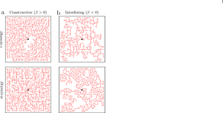
Figure 3: Patterns of infection. Illustration of the effect of (a) constructive and (b) interfering synergy on the patterns of infection spreading from the central host (marked by solid circle) in systems of linear size $L=31$. The synergy rates are $\beta=5$ and $\beta=-5$ for patterns with constructive and interfering synergy, respectively. All snapshots correspond to the final state of the epidemic with only R and S hosts remaining. Solid lines indicate those edges between d-r pairs that have transmitted the pathogen at some time during the course of the epidemic. The value of $\alpha$ has been chosen in each case such that the probability of invasion is $P_{\text{inv}}=0.5$ for all snapshots: (a) $\alpha=0.47$ for r-synergy and $\alpha=0.18$ for d-synergy. (b) $\alpha=0.81$ for r-synergy and $\alpha=5.22$ for d-synergy.

Figure 4: Branching and invasion transitions for d-synergy. (a) Diagram showing the branching transition line $\alpha_{\text{b}}(\beta)=-\beta$ together with the phase boundary for invasion/non-invasion transition, $\alpha_{\text{c}}(\beta)$. Branching is forbidden in the region under the continuous line where $\alpha<\alpha_{\text{c}}(\beta)$. Invasive epidemics can occur in the region above the dashed line corresponding to $\alpha>\alpha_{\text{c}}(\beta)$ where branching is present. The intermediate region between the continuous and dashed lines with $\alpha_{\text{b}}<\alpha<\alpha_{\text{c}}$ corresponds to epidemics that display branching but are not invasive. (b) Example of path for infection with d-synergy in the regime without branching ($\alpha\leq\alpha_{\text{b}}$). Infection starts from the host marked by a solid circle and evolves along the path indicated by arrows. Arrow numbers define schematically a sequence of infection events. For the first infected host (solid circle), $n_{\text{d}}=0$ and infection can be transmitted to any of its neighbours at a rate $\lambda_{\text{d-r}}=\alpha$. However, $n_{\text{d}}=1$ as soon as the pathogen is transmitted to one of the neighbours (arrow 1) and thus $\lambda_{\text{d-r}}=0$ because $\alpha\leq-\beta$. At this moment, transmission of infection is arrested until the initially infected host recovers. After this recovery, $n_{\text{d}}=0$ for the newly infected host and infection can be transmitted to one of its nearest neighbours at rate $\alpha$. Iteration of this process over time gives growing SAWs. The state after the event marked by arrow 10 illustrates the phenomenon of self-trapping.

As a measure of the temporal efficiency for invasion, we consider the time, $t_{\text{inv}}$, it takes for the pathogen to invade the system. Numerical simulations (see Appendix D) show that for any given value of $P_{\text{inv}}$, the time $t_{\text{inv}}$ decreases with increasing $\beta$ (for both types of synergy). Therefore, systems with interfering synergy are less time-efficient than those with constructive synergy. The largest deviations of $t_{\text{inv}}$ from its value without synergy are obtained for epidemics with d-synergy that operates in every transmission event.

The analysis presented above demonstrates that synergy in transmission of infection has significant and sometimes paradoxical and unexpected effects on epidemics. Despite the simple assumptions of the model (such as, e.g., short-range synergy and linear dependence of the rate of infection on the number of infected nearest neighbours), it reproduces explorative and exploitative foraging strategies that are typically observed in bacterial, fungal, and tumour growth Rayner_Mycologia1991_review ; Ferreira_PRE2002 ; Ben-Jacob_Nature1994 . The explorative/exploitative behaviour in our model is linked to interfering/constructive synergy. The foraging strategy adopted by fungi, bacteria or ants is known to be explorative/exploitative when resources are limited/abundant.

Changes in the foraging strategy are ultimately due to the spatial correlations in transmission rates emerging as a consequence of synergy. Spatial correlations in $\lambda_{\text{\text{d-r}}}$ appear because the neighbourhood of sufficiently close pairs of hosts have common nodes and thus the rates for each pair are not mutually independent. Synergistic epidemics can then be regarded as a correlated dynamical percolation analogous to the well-known mapping of the non-synergistic SIR process to uncorrelated dynamical percolation (see  Grassberger1983 ; Henkel_Hinrichsen_Book2009 ; Sander et al. (2002); PerezReche_JRSInterface2010 and details on the mapping to correlated dynamical percolation in Appendix E). In most situations, spatial correlations in transmission are short-ranged and the critical behaviour of epidemics at $\alpha_{\text{c}}$ belongs to the dynamical uncorrelated bond-percolation universality class Grassberger1983 ; Henkel_Hinrichsen_Book2009 . However, for large interfering d-synergies with $\alpha<\alpha_{\text{b}}(\beta)$ (region under continuous line in Fig. 4(a)) correlations become effectively long-ranged and epidemics are growing SAWs whose critical properties belong to the universality class of the standard SAW Pietronero_PRL1985 ; Hemmer_PRA1986 . Although the SAW behaviour affects the local properties of epidemics with $\alpha\gtrsim\alpha_{\text{b}}(\beta)$, the large-scale behaviour at $\alpha_{\text{c}}$ is not affected (i.e. the critical exponents at invasion are the same as those for uncorrelated bond percolation, as shown in detail in Appendix B). This is a consequence of the fact that the probability that a growing SAW invades a large system is known to be zero due to the self-trapping phenomenon Pietronero_PRL1985 ; Hemmer_PRA1986 . This implies that $\alpha_{\text{c}}>\alpha_{\text{b}}$ for any value of $\beta$ (cf. Fig. 4(a)).

The proposed model becomes analytically tractable if spatial correlations in transmission are assumed to be negligible. The analytic solutions provide a good qualitative description of the main features of the phase diagram for both r- and d-synergy. Correlations in the exact model prevent the approximate description from being quantitative (cf. Appendix F for a complete description).

In summary, the presented work shows that synergistic effects at the individual level play an important role in invasion at the population level. The analysis has been restricted to the spread of epidemics in 2D regular networks relevant for, e.g., populations of plants in a field. The extension of our work to synergistic effects for spreading processes in higher-dimensional lattices or more complex networks is not only conceptually appealing but also important for problems in multiple disciplines Note4 . Although such an extension is technically straightforward, understanding the interplay between synergistic effects and topological properties for different types of networks is a challenging task for future work.

Appendices

Appendix A Probability of invasion

In this section, we discuss the dependence of the probability of invasion, $P_{\text{inv}}$, on the rates $\alpha$ and $\beta$. The probability of invasion is defined as the relative number of invasive events out of many (in our simulations, $\gtrsim 5000$) stochastic realizations of epidemics. Although we will deal with systems of finite size, the trends of $P_{\text{inv}}$ (see Fig. 5) are in qualitative agreement with those expected from the phase diagram for epidemics in infinite systems shown in the main text (Fig. 2). For both r- and d-synergy, the invasion curves ($P_{\text{inv}}$ vs $\alpha$) approach zero for small transition rates $\alpha$ thus describing the non-invasive regime for epidemics. For large values of $\alpha$, the invasion probability is finite so that it describes the invasive regime. The invasion curves start to deviate from zero at progressively lower values of $\alpha$ as $\beta$ increases. This illustrates the non-increasing character of $\alpha_{\text{c}}(\beta)$ for increasing $\beta$ discussed in the main text. The tendencies of $P_{\text{inv}}$ in extreme situations require further explanations that are different for r- and d-synergy.

Figure 5: Probability of invasion $P_{\text{inv}}$ in a system of linear size $L=31$ as a function of the elementary rate $\alpha$ for (a) r-synergy and (b) d-synergy. Different curves correspond to different values of the synergy rate, $\beta$, as indicated in the legend for each case.

r-synergy

Fig. 5(a) shows the probability of invasion for epidemics with r-synergy in systems of linear size $L=31$ as a function of $\alpha$ (invasion curves) for several values of $\beta$. For large positive values of $\beta$, the invasion curves tend to a single (master) curve which can be described by a limiting function of $\alpha$ that does not depend significantly on $\beta$. This is illustrated in Fig. 5(a) by two curves for $\beta=50$ and $\beta=100$ coinciding within numerical error. Consequently, on the phase diagram, the critical line $\alpha_{\text{c}}(\beta)$ tends towards the limiting value $\alpha_{\text{c}}(\infty)\simeq 0.2$ (shown by the arrow in Fig. 2, main text). In cases with large interference in transmission (corresponding to very negative $\beta$), the curves for $P_{\text{inv}}(\alpha)$ again collapse on a limiting curve shown in Fig. 5(a) for $\beta=-1.5$ and $\beta=-2.0$. The corresponding invasion threshold in the thermodynamic limit is located at $\alpha_{\text{c}}=0.86\pm 0.01$ independently of the value of $\beta$.

d-synergy

For d-synergy and values of $\beta\gtrsim 0.8$, invasion is possible for any positive value of $\alpha$. In this regime, the invasion curves collapse on a master curve that does not depend on the value of $\beta$ (cf. curves in Fig. 5(b) for $\beta=5$ and $\beta=50$). For negative values of $\beta$, the invasion curves do not approach a limiting function as $\beta$ decreases (Fig. 5(b)). As a result, $\alpha_{\text{c}}$ increases monotonically with decreasing $\beta$ (see Fig. 2, main text).

Appendix B Critical behaviour and finite-size effects

In this section, we give details about the methods used for obtaining the phase diagram for invasion in the limit $L\rightarrow\infty$ (see Fig. 2 in the main text). In addition, we give numerical support for the statements made in the main text about the critical behaviour displayed by epidemics with d-synergy in the different regions presented in Fig. 4(a) of the main text.

The data points for the phase boundary, $\alpha_{\text{c}}(\beta)$, in the phase diagram for invasion were obtained by analysing both the probability of invasion, $P_{\text{inv}}$, and the average relative number, $N_{1}$, of epidemics spanning the system in one and only one direction (1D-spanning epidemics). The analysis of $N_{1}$ presented here is similar to that performed for avalanches in spin models with quenched disorder Pérez-Reche and Vives (2003); Pérez-Reche et al. (2008).

Below we show that, for epidemics with constructive or weakly interfering synergy, the method based on the analysis of 1D-spanning clusters gives more accurate estimates for $\alpha_{\text{c}}(\beta)$ than those obtained by using $P_{\text{inv}}$. In particular, our estimates for the invasion threshold for non-synergistic epidemics based on $N_{1}$ are in excellent agreement with the value $\alpha_{\text{c}}(0)=\tau^{-1}\ln 2$ expected from the mapping to bond-percolation valid for $\beta=0$ . In contrast, for epidemics with large interfering d-synergy, the estimation of $\alpha_{\text{c}}(\beta)$ based on $P_{\text{inv}}$ is more accurate than that achieved by using $N_{1}$.

B.1 Epidemics with constructive or weakly interfering synergy

Figure 6: (a) Dependence of the average relative number of 1D-spanning epidemics, $N_{1}$, on the elementary rate $\alpha$ for d-synergy with $\beta=0.3$. Different curves correspond to systems of different size $L$, as marked in the legend. (b) Scaling collapse of $N_{1}$ according to the scaling law (2) for the curves shown in (a). The critical exponents have been set to the values $\nu=4/3$ and $\beta=5/36$, corresponding to values found for uncorrelated percolation. The scaling collapse gives the invasion threshold $\alpha_{\text{c}}=0.445\pm 0.005$.

For epidemics with constructive or weakly interfering synergy, the quantity $N_{1}$ has a peak when plotted as a function of $\alpha$ for a fixed value of $\beta$. This is the case for both r- and d-synergy. Fig. 6 shows a representative example corresponding to constructive d-synergy with $\beta=0.3$. The position of the peak for $N_{1}$ is related to the critical value of the parameter $\alpha$ separating invasive and non-invasive regimes. Indeed, in the non-invasive regime, $N_{1}\simeq 0$ because the clusters of removed hosts are of small size and thus they have a negligible probability to touch the boundaries of a finite system. On the other hand, $N_{1}$ is expected to be close to zero in the invasive regime as well because the pathogen spreads in two directions rather than along one only. As a result, $N_{1}$ can be finite at the invasion threshold or, due to finite-size effects, in a certain region around the threshold. The critical value $\alpha_{\text{c}}(\beta)$ in the limit $L\rightarrow\infty$ is obtained using the scaling properties of $N_{1}(\alpha,L)$ in the vicinity of the invasion threshold. Due to the absence of characteristic length scales at criticality, the dependence of $N_{1}$ on $\alpha$ and $L$ is expected to obey the following scaling law Pérez-Reche and Vives (2003); Pérez-Reche et al. (2008):

$$N_{1}(\alpha,L)=L^{\theta}\tilde{N}_{1}((\alpha-\alpha_{\text{c}})L^{1/\nu})~{},$$ (2)

where $\theta$ and $\nu$ are critical exponents and $\tilde{N}_{1}$ is a scaling function which depends on $\alpha$ and $L$ through the product $(\alpha-\alpha_{\text{c}})L^{1/\nu}$ only. The values of $\theta$, $\nu$, and $\alpha_{\text{c}}$ can be determined by scaling collapse for $N_{1}(\alpha,L)$. Technically, this can be achieved by plotting the quantity $L^{-\theta}N_{1}$ vs $(\alpha-\alpha_{\text{c}})L^{1/\nu}$ and requiring that the scaling hypothesis (2) is satisfied (i.e. curves for different $L$ collapse on a single master curve corresponding to $\tilde{N}_{1}$). Fig. 6(b) shows an example of such scaling collapse for d-synergy with $\beta=0.3$. In this case, the collapse gives the values $\alpha_{\text{c}}=0.445\pm 0.005$ and $\theta=-0.10\pm 0.05$. Bearing in mind the mapping of SIR epidemics to dynamical uncorrelated bond-percolation holding for $\beta=0$ Grassberger1983 , the value of $\nu$ has been fixed to $\nu=4/3$ corresponding to uncorrelated percolation Stauffer and Aharony (1994). The good quality of the collapse suggests that, despite the existence of correlations in transmission of infection for $\beta\neq 0$, the critical behaviour at $\alpha_{\text{c}}(\beta)$ falls into the universality class for the uncorrelated percolation. This is the expected behaviour when correlations are short-ranged Isichenko (1992).

Figure 7: (a) Dependence of the probability of invasion, $P_{\text{inv}}$, on the elementary rate $\alpha$ for d-synergy with $\beta=0.3$. Different curves correspond to systems of different size $L$, as marked in the legend. (b) Scaling collapse of $P_{\text{inv}}$ according to the scaling law given by Eq. (3) for the curves shown in (a). The critical exponents have been set to the values $\nu=4/3$ and $\beta=5/36$. The invasion threshold has been set to the value $\alpha_{\text{c}}=0.445$ obtained from the collapse of $N_{1}$ (cf. Fig. 6).

The above statement is also supported by the behaviour of $P_{\text{inv}}$ in the vicinity of the invasion threshold which satisfies the following scaling hypothesis,

$$P_{\text{inv}}=L^{-\beta/\nu}\tilde{P}_{\text{inv}}((\alpha-\alpha_{\text{c}})L^{1/\nu}),$$ (3)

with the exponents $\nu=4/3$ and $\beta=5/36$ corresponding to uncorrelated percolation. As an example, Fig. 7(b) shows the scaling collapse for the curves shown in Fig. 7(a) for several system sizes. The collapse in Fig. 7(b) has been obtained by setting $\alpha_{\text{c}}$ to the value $\alpha_{\text{c}}=0.445$ obtained from the collapse of $N_{1}$. The quality of this collapse is remarkably good despite the fact that no free parameters have been used (i.e. the value of $\nu$, $\beta$, and $\alpha_{\text{c}}$ has been considered as being fixed).

If instead of fixing $\alpha_{\text{c}}$, we try to estimate its value from the collapse of $P_{\text{inv}}$, the sigmoidal shape of $P_{\text{inv}}$ prevents the estimate from being as accurate as the one obtained from the collapse of $N_{1}(\alpha,L)$ which are peak-shaped.

B.2 Epidemics with large interfering d-synergy

In the main text, we have shown that epidemics with interfering d-synergy behave as growing self-avoiding walks (SAWs) for $\alpha\leq\alpha_{\text{b}}=-\beta$ (cf. Fig. 4(a), main text). Fig. 8(a) shows $N_{1}$ vs $\alpha$ for epidemics with $\beta=-10$ spreading in systems of different size. As can be seen, growing SAWs give a constant contribution to $N_{1}$ for $\alpha\leq 10=\alpha_{\text{b}}(\beta)$. The probability that a growing SAW spans the system in one dimension decreases with the system size, $L$, and thus the contribution of such objects to $N_{1}$ tends to zero as $L\to\infty$. In our simulations, the systems are finite and contribution of the 1D SAWs to $N_{1}$ is not negligible. As a consequence, the scaling collapses of $N_{1}$ based on the hypothesis by Eq. (2) are of low quality and not very useful for the estimation of $\alpha_{\text{c}}(\beta)$ for some negative values of $\beta$.

Figure 8: (a) Dependence of the average relative number of 1D-spanning epidemics, $N_{1}$, on the elementary rate $\alpha$ for d-synergy with $\beta=-10.0$. Different curves correspond to systems of different size $L$, as marked in the legend. (b) Scaling collapse of $N_{1}$ according to the scaling law given by Eq. (2) for the curves shown in (a). The critical exponents have been set to the values $\nu=4/3$ and $\beta=5/36$. The invasion threshold has been set to the value $\alpha_{\text{c}}=10.15$ obtained from the collapse of $P_{\text{inv}}$ (cf. Fig. 9).

Figure 9: (a) Dependence of the probability of invasion, $P_{\text{inv}}$, on the elementary rate $\alpha$ for d-synergy with $\beta=-10$. Different curves correspond to systems of different size $L$, as marked in the legend. (b) Scaling collapse of $P_{\text{inv}}$ according to the scaling law given by Eq. (3) for the curves shown in (a). The critical exponents have been set to the values $\nu=4/3$ and $\beta=5/36$, corresponding to uncorrelated percolation. The scaling collapse gives the invasion threshold $\alpha_{\text{c}}=10.15\pm 0.03$.

In this situation, the estimates of the critical values of the rate $\alpha$ are more conveniently obtained by analysing the probability of invasion, $P_{\text{inv}}$. This quantity is less affected by the growing SAW epidemics because invasion requires reaching all the four edges of the system. Fig. 9(a) shows the dependence of $P_{\text{inv}}$ on $\alpha$ for $\beta=-10$. Fig. 9(b) demonstrates the scaling collapse of the curves displayed in panel (a) with the exponents $\nu=4/3$ and $\beta=5/36$ corresponding to uncorrelated percolation and $\alpha_{\text{c}}=10.15\pm 0.03$. The quality of the collapse suggests that, despite the proximity of $\alpha_{\text{c}}$ to $\alpha_{\text{b}}$, the behaviour at large scales corresponds to that of dynamical uncorrelated percolation. Use of the same value of the critical rate, $\alpha_{\text{c}}=10.15$, for $N_{1}(\alpha,L)$ results in a collapse of much poor quality (see Fig. 8). As expected, the quality of the collapse is reasonable only for relatively large values of $(\alpha-\alpha_{c})L^{1/\nu}$ for which the influence of growing SAWs is negligible.

Appendix C Mean spatial density of invasion

In this section, we give further quantitative support to the results discussed in the main text concerning the effect of synergy on the spatial density of invasion. The mean spatial density of invasion is defined as the relative number of hosts, $n_{\text{R}}$, that are in the removed state (R) by the end of an invasive epidemic (i.e. the relative number of hosts that have been infected during the course of the epidemic and are removed by the end). Due to stochasticity in the transmission of infection, different realisations of invasive epidemics characterised by the same parameters $\alpha$ and $\beta$ have a different random value for $n_{\text{R}}$. The probability density function for the density of infection, $\rho(n_{\text{R}})$, has a single peak for any values of the parameters $\alpha$ and $\beta$ (see the inset in Fig. 10). Therefore, $n_{\text{R}}$ has a well-defined scale that, due to the small degree of asymmetry of $\rho(n_{\text{R}})$, can be properly represented by the mean $\langle n_{\text{s}}\rangle$ with dispersion given by the standard deviation. Fig. 10 shows the dependence of the spatial efficiency on $\beta$ for invasive epidemics with value of $\alpha$ chosen in each case so that $P_{\text{inv}}=0.5$. As stated in the main text, the mean density of invasion exhibits a global tendency to increase with increasing $\beta$ both for r- and d-synergy.

As expected, $n_{\text{R}}$ is identical for the two types of synergy if $\beta=0$. For any non-zero value of $\beta$, the density of infection for d-synergy, $n_{\text{R,d}}$, is larger than that for r-synergy, $n_{\text{R,r}}$. In cases with constructive synergy, it is likely that $n_{\text{R,d}}\geq n_{\text{R,r}}$ because, as argued in the main text, synergistic effects are more prominent for d-synergy (they operate in every transmission event). A plausible explanation for the origin of the inequality $n_{\text{R,d}}>n_{\text{R,r}}$ for $\beta<0$ can be given by recalling that branching is more frequent in paths of infection for r-synergy than for d-synergy. Due to the higher degree of branching for r-synergy, it is more probable that hosts become effectively isolated from infection for this type of synergy if they are simultaneously challenged by several neighbours which interfere and do not transmit infection. As an extreme case, consider a situation in which a host is simultaneously challenged by its all four neighbours. It is clear that the challenged host will become inaccessible forever if infection is not transmitted by any of the four challenging neighbours. In contrast, the lower degree of branching for d-synergy makes the existence of effectively isolated hosts less likely. As a consequence, more hosts can be infected for d-synergy during the course of epidemics.

Figure 10: Mean density of invasion, $n_{\text{R}}$, as a function of $\beta$ for epidemics with $P_{\text{inv}}=0.5$ in systems of linear size $L=31$. Symbols (squares for r-synergy and circles for d-synergy) correspond to the mean of $n_{\text{R}}$ over stochastic realisations and error bars show the standard deviation. The inset displays representative examples of the probability density function for the mean density of invasion, $\rho(n_{\text{R}})$, for $\beta=-2$.

Appendix D Temporal efficiency

This section complements the part of the main text devoted to the time to invasion, $t_{\text{inv}}$. Due to stochasticity in the transmission of infection, $t_{\text{inv}}$ is a random variable described by a probability density function, $\rho(t_{\text{inv}})$, which has a single peak for any values of the parameters $\alpha$ and $\beta$ (see the inset in Fig. 11). We can then proceed in an analogous manner as we have done above for the mean density of infection and describe $t_{\text{inv}}$ by its mean $\langle t_{\text{inv}}\rangle$ and dispersion given by the standard deviation. Fig. 11 shows that for both types of synergy $\langle t_{\text{inv}}\rangle$ decreases with increasing $\beta$. The dispersion of $\rho(t_{\text{inv}})$ also decreases with increasing $\beta$, as indicated by the error bars in Fig. 11.

By definition, the time to invasion is identical for the two types of synergy if $\beta=0$. For $\beta\neq 0$, the largest deviations of $t_{\text{inv}}$ from its value without synergy ($\beta=0$) (cf. circles and squares in Fig. 11) are for epidemics exhibiting d-synergy. This is mostly due to the fact that d-synergy operates in every transmission event. In average, this makes transmission events slower/quicker for interfering/constructive d-synergy. In addition to this factor, it is likely that the higher degree of branching in the foraging strategy for infection with interfering r-synergy also contributes to making $t_{\text{inv}}$ smaller for r-synergy with $\beta<0$.

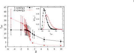
Figure 11: Time to invasion, $t_{\text{inv}}$, as a function of $\beta$ for epidemics with $P_{\text{inv}}=0.5$ in systems of linear size $L=31$. Symbols (squares for r-synergy and circles for d-synergy) correspond to the mean of $t_{\text{inv}}$ and error bars show the standard deviation. The inset displays representative examples of the probability density function for the time to invasion, $\rho(t_{\text{inv}})$, for $\beta=-2$.

Appendix E Invasion as a correlated dynamical bond-percolation problem

The aim of this section is twofold. First, we give detailed definitions for the transmissibility in synergistic epidemics and related quantities such as its probability density function (p.d.f.) and mean value. Second, the effect of correlations on the probability of invasion summarised in the main text is analysed here in more detail.

E.1 Transmissibility

In the presence of synergistic effects, the transmission of infection can be described as a non-homogeneous Poisson process with the time-dependent infection rate $\lambda_{\text{d-r}}(t)$ defined by Eq. (1) in the main text. The probability that the infection has not been transmitted in a d-r (donor-recipient) pair by time $t$ defines the survival probability $S_{\text{d-r}}(t)$. For a non-homogeneous Poisson process, $S_{\text{d-r}}(t)$ satisfies the following differential equation Ludwig (1975); Pellis et al. (2008):

$$\frac{\text{d}S_{\text{d-r}}}{\text{d}t}=-\lambda_{\text{d-r}}(t)S_{\text{d-r}}(t)~{}.$$

The solution of this equation with initial condition $S(t=0)=1$ (such a condition ensures that the pathogen is not transmitted instantaneously when the donor is infected) is

$$S_{\text{d-r}}(t)=\exp\left[-\int\limits_{0}^{t}\lambda_{\text{d-r}}(t)~{}\text{d}t\right]~{}.$$ (4)

The transmissibility $T_{\text{d-r}}$ is defined as the probability that the pathogen is transmitted from the donor to the recipient over the infectious period of the donor, $\tau$. Therefore, it can be expressed in terms of the survival probability as follows:

$$T_{\text{d-r}}=1-S_{\text{d-r}}(\tau)~{}.$$ (5)

Substitution of the expression for $S_{\text{d-r}}$ given by Eq. (4) into Eq. (5) results in the following expression for $T_{\text{d-r}}$:

$$T_{\text{d-r}}=1-\exp\left(-\int_{0}^{\tau}\lambda_{\text{\text{d-r}}}(t)\,\text{d}t\right)~{}.$$ (6)

In the absence of synergistic effects, the rate $\lambda_{\text{d-r}}(t)=\alpha$ remains constant over the infectious period $\tau$ and is the same for all d-r pairs. In this case, the transmissibility reduces to the homogeneous value, $T_{\text{d-r}}=1-e^{-\tau\alpha}$, that plays a central role in the mapping of SIR epidemics to the well-known uncorrelated dynamical percolation Grassberger1983 ; Henkel_Hinrichsen_Book2009 . In this mapping, $T_{\text{d-r}}$ is identified with the bond probability and $P_{\text{inv}}$ from an initially inoculated site is identified with the probability $P_{\infty}$ that such site belongs to the infinite cluster of connected sites in the dynamical percolation problemStauffer and Aharony (1994). For SIR epidemics, $P_{\text{inv}}$ is fully parameterised by $T_{\text{d-r}}$. This is analogous to the fact that $P_{\infty}$ is fully parameterised by the bond probability in dynamical percolation.

When synergy is present, the transmissibility $T_{\text{d-r}}$ is a functional that depends on the time evolution of the rate $\lambda_{\text{d-r}}(t)$ which, in turn, depends on the infection history of the neighbouring hosts to the d-r pair. Each d-r pair involved in an epidemic is in general characterised by a different dependence of the rate $\lambda_{\text{d-r}}(t)$ on time. As a consequence, the field of transmissibilities is spatially heterogeneous. In addition, the dependence of $T_{\text{d-r}}$ on the neighbourhood of the d-r pair introduces non-trivial correlations in transmission and thus in transmissibilities.

In order to study the role of synergy-induced correlated heterogeneity at the host level on $P_{\text{inv}}$ we proceed in a way inspired from previous works dealing with heterogeneous SIR epidemics Kuulasmaa (1982); Cox and Durrett (1988); Kenah2007 ; Miller_JApplProbab2008; Neri et al. (2011); Handford et al. (2011). The simplest situation with heterogeneity in transmission corresponds to epidemics where $T_{\text{d-r}}$ are independent random variables for all d-r pairs. In this case, $P_{\text{inv}}$ only depends on the mean transmissibility, $\langle T\rangle$ Sander et al. (2002); PerezReche_JRSInterface2010 . In more complicated situations, the transmissibilities for different d-r pairs are not independent and $P_{\text{inv}}$ is a function of the whole set of transmissibilities, $\{T_{\text{d-r}}\}$, that cannot be completely parametrised by $\langle T\rangle$ Kuulasmaa (1982); Cox and Durrett (1988); Kenah2007 ; Miller_JApplProbab2008; Neri et al. (2011); Handford et al. (2011). An exact mapping of such SIR epidemics to uncorrelated percolation is not possible in general. However, the use of $\langle T\rangle$ can still be useful to analyse the consequences that heterogeneity in local transmission has on $P_{\text{inv}}$. For instance, a considerable progress has been made in understanding the role of correlations in epidemics where heterogeneity in transmission is associated with heterogeneity in recovery times of infected hosts. In this case, the following important result has been rigorously derived Kuulasmaa (1982); Cox and Durrett (1988); Neri et al. (2011): for a given value of $\langle T\rangle$, the resilience to invasion increases with increasing degree of heterogeneity (more precisely, $P_{\text{inv}}^{\text{het}}(\langle T\rangle)\leq P_{\text{inv}}^{\text{hom}}(\langle T\rangle)$, where $P_{\text{inv}}^{\text{het}}$ and $P_{\text{inv}}^{\text{hom}}$ are the probabilities of invasion for heterogeneously and homogeneously distributed removal times, respectively). Here, we show that the dependence of $P_{\text{inv}}$ on $\langle T\rangle$ for synergistic epidemics is more complicated (see Fig. 12). In spite of that, in subsections E.2 and E.3 we show that analysing the dependence of $P_{\text{inv}}$ on the degree of synergy for given $\langle T\rangle$ is still informative.

For synergistic epidemics we define the mean transmissibility in terms of two averages: spatial average in each realisation of epidemics and stochastic over different epidemic realisations. The spatial average for transmissibility, $\overline{T}_{r}$, is calculated for a particular $r$-th realisation of the epidemic in the following manner,

$$\overline{T}_{r}=\frac{1}{N_{\text{d-r}}}\sum_{\text{d-r}}T_{\text{d-r}}~{},$$

where the sum extends over the number $N_{\text{d-r}}$ of d-r pairs in the final state of the epidemic, i.e. over all d-r pairs challenged by the infection. The value of $T_{\text{d-r}}$ in the above equation for each d-r pair is calculated using Eq. (6) with the transmission rate $\lambda_{\text{d-r}}(t)$ measured numerically for the $r$-th realisation of epidemic. The direct numerical evaluation of the transmissibility for synergistic epidemics as a frequency of successful transmission of infection between donor and recipient in the d-r pair would require reproduction of time-dependent transmission rates giving exactly the same integral over time, $-\int_{0}^{\tau}\lambda_{\text{d-r}}(t)\text{d}t$ (i.e. all possible rates $\lambda_{\text{d-r}}(t)$ giving the same value of $T_{\text{d-r}}$ in Eq. (6)). This imposes a very restrictive condition on the time of infection of the nodes in the neighbourhood of the d-r pair and thus evaluation of $T_{\text{d-r}}$ as a frequency can be hardly a feasible computational task. The mean transmissibility, $\langle T\rangle$, is obtained by stochastic averaging of $\overline{T}_{r}$ for $R$ different realisations of the epidemic:

$$\langle T\rangle=\frac{1}{R}\sum_{r=1}^{R}\overline{T}_{r}~{},$$

where the value of $\overline{T}_{r}$ is averaged over $R$ different stochastic realisations of the epidemic. Note that averaging over stochastic realisations is necessary to account for the fact that different realisations of epidemics lead to different spatial configurations for $\{T_{\text{d-r}}\}$.

Bearing in mind that the population of hosts is homogeneous (i.e. $\alpha$ and $\beta$ do not depend on the d-r pair location) the values of transmissibilities for any d-r pair given by Eq. (6) are independent random variables characterized by a p.d.f., $\rho(T_{\text{d-r}})$. Once $\rho(T_{\text{d-r}})$ is available, e.g. numerically, the mean transmissibility can equivalently be calculated as

$$\langle T\rangle=\int_{0}^{1}T\rho(T)\,\text{d}T~{}.$$ (7)

The analysis of $\rho(T_{\text{d-r}})$ is important for understanding the dependence of $P_{\text{inv}}$ on the degree of synergy and $\langle T\rangle$, as we show below for r- and d-synergy.

E.2 r-synergy

Fig. 12 shows the dependence of $P_{\text{inv}}$ on $\langle T\rangle$ for several values of $\beta$. For any fixed value of $\langle T\rangle$, the probability of invasion with interfering synergy (see the curves corresponding to $\beta<0$ and marked by open and solid circles and open squares in Fig. 12) is systematically greater than for non-synergistic epidemics (see the curve for $\beta=0$ marked by solid circles in Fig. 12), i.e. the populations exhibiting interfering r-synergy are more vulnerable to invasion than those without synergy. For constructive r-synergy, it is possible to distinguish between two different regimes. The first regime corresponds to epidemics with moderate synergy (curves for $\beta=0.8\;\text{and}\;2$ in Fig. 12) that are less invasive than non-synergistic epidemics for all values of $\langle T\rangle$, i.e. the curves marked by the solid diamonds and stars are always below the curve marked by the solid squares. The second regime corresponds to larger values of $\beta$ (e.g. $\beta=50\;\text{and}\;100$ in Fig. 12). In this case, there is a range of $\langle T\rangle$ where the curves marked by open triangles and crosses are above the curve marked by the solid squares. In this interval for $\langle T\rangle$, the epidemics with constructive r-synergy are more invasive than those without synergy.

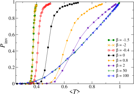
Figure 12: Probability of invasion as a function of the mean transmissibility for r-synergy in systems of linear size $L=31$. Different curves correspond to different values of $\beta$ as marked in the figure.

These features can be qualitatively illustrated by analysing the evolution of the distribution of transmissibilities, $\rho(T_{\text{d-r}})$, with the strength of synergy. Without synergy, $\rho(T_{\text{d-r}})$ has a $\delta$-functional shape, $\rho(T_{\text{d-r}})=\delta(T_{\text{d-r}}-T_{1})$, where $T_{1}=1-e^{-\alpha\tau}$ is the non-synergistic transmissibility. The epidemic is invasive (non-invasive) if $T_{1}>T_{c}=1/2$ ($T_{1}\leq T_{c}$) Grassberger1983 . Once r-synergy is introduced, the shape of $\rho(T_{\text{d-r}})$ changes. The $\delta$-functional peak is still present and it describes recipients with a single infected neighbour, $n_{\text{r}}=1$. In addition, new contributions to $\rho(T_{\text{d-r}})$ appear for $T_{\text{d-r}}<T_{1}$ ($T_{\text{d-r}}>T_{1}$) in case of negative (positive) values of $\beta$ (see the lower panel in Fig. 13 where the $\delta$-functional peak at $T_{\text{d-r}}=T_{1}$ is marked by $\diamond$). Such contributions come from recipients surrounded by more than one infected neighbour, i.e. $n_{\text{r}}>1$. The number of infected neighbours varies in discrete manner and this brings a non-smooth functional dependence to $\rho(T_{\text{d-r}})$ consisting of cusps associated with the discrete changes in $n_{\text{r}}(t)$ and smooth components between cusps originated from the continuity of time. In other words, $n_{\text{r}}(t)$ is a piece-wise function of time the integral of which produces a continuous set of transmissibilities according to Eq. (6).

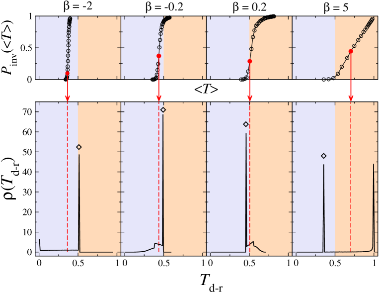
Figure 13: The upper panels show $P_{\text{inv}}$ vs. $\langle T\rangle$ for four values of $\beta$ for r-synergy. The lower panels show the p.d.f. $\rho(T_{\text{d-r}})$ corresponding to the points in the invasion curves indicated in the upper panels with an arrow. The mean of the p.d.f. $\rho(T_{\text{d-r}})$ gives the value of $\langle T\rangle$ in the upper panel (Eq. (7)). The non-synergistic transmissibility $T_{1}=1-e^{-\alpha\tau}$ corresponding to the recipients with $n_{\text{r}}=1$ is marked by $\diamond$ in all the panels. The critical transmissibility for non-synergistic epidemics is $T_{c}=1/2$. The intervals of transmissibility with $T<T_{c}$ and $T>T_{c}$ are indicated by the blue and orange shaded regions, respectively.

For interfering synergy, the average transmissibility is $\langle T\rangle<T_{1}$, due to the contribution to $\rho(T_{\text{d-r}})$ of $T_{\text{d-r}}<T_{1}$ described above. If the heterogeneous transmissions associated with synergy were uncorrelated, the probability of invasion for synergistic epidemics with the elementary rate $\alpha$ would be smaller than that corresponding to epidemics with the same value of $\alpha$ but without synergy. This is a consequence of the fact that the probability of invasion for systems with heterogeneous but uncorrelated transmissions depends on $\langle T\rangle$ only Cox and Durrett (1988); Sander et al. (2002); PerezReche_JRSInterface2010 . However, this is not the case for epidemics with interfering synergy which are more invasive than epidemics without synergy. This is due to correlations between synergistic transmissibilities. Indeed, the d-r pairs that passed the infection in an epidemic (mostly those with non-synergistic transmissibility $T_{1}$) are arranged in a spatially correlated finger-like manner (as shown in Fig. 3(b) in the main text) that makes invasion possible. Therefore, the synergistic epidemics can be mapped onto the correlated dynamical bond-percolation problem in which the bond probabilities are associated with transmissibilities.

For constructive synergy with moderate values of $\beta$ (corresponding to the first regime mentioned above), most of the d-r pairs in the system have transmissibility $T_{1}<T_{\text{c}}=1/2$ (cf. the position of the peak marked by $\diamond$ with the rest of the distribution in the panel for $\beta=0.2$ in Fig. 13). Most of the synergistic d-r pairs have $T_{\text{d-r}}>T_{c}$ as can be seen from the comparison of the areas under the curve for p.d.f. for $T_{\text{d-r}}<T_{c}$ (excluding non-synergistic transmissibilities under the peak marked by $\diamond$) and $T_{\text{d-r}}>T_{c}$. However, the abundance and value of the transmissibilities for such synergistic pairs does not seem to be high enough as to allow for invasion unless $\langle T\rangle$ is clearly larger than $T_{c}$.

For larger values of $\beta$, invasion is possible for $\langle T\rangle<T_{\text{c}}$ because, as shown in Fig. 13 for $\beta=5$, the relative number of synergistic pairs is large enough and they have $T\simeq 1$ so that the transmission of infection is very likely. Moreover, these pairs are placed in a spatially correlated manner which also favours the invasion for $\langle T\rangle<T_{\text{c}}$.

E.3 d-synergy

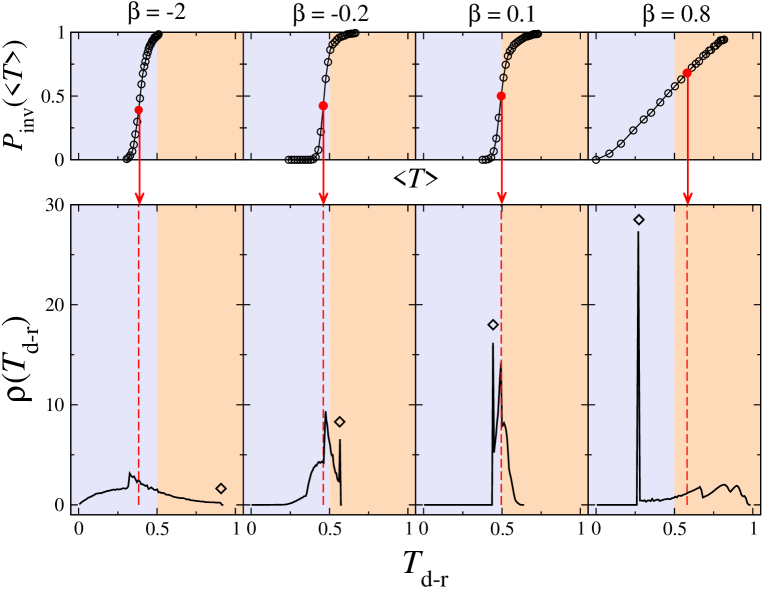
Figure 14: The upper panels show $P_{\text{inv}}$ vs. $\langle T\rangle$ for four values of $\beta$ for d-synergy. The lower panels show the p.d.f. $\rho(T_{\text{d-r}})$ corresponding to the points in the invasion curves indicated in the upper panels with an arrow. The mean of the p.d.f. $\rho(T_{\text{d-r}})$ gives the value of $\langle T\rangle$ in the upper panel (Eq. (7)). The non-synergistic transmissibility $T_{0}=1-e^{-\alpha\tau}$ corresponding to recipients with $n_{\text{d}}=0$ is marked by $\diamond$ in all the panels. The critical transmissibility for non-synergistic epidemics is $T_{c}=1/2$. The intervals of transmissibility with $T<T_{\text{c}}$ and $T>T_{\text{c}}$ are indicated by the blue and orange shaded regions, respectively.

The p.d.f. $\rho(T_{\text{d-r}})$ for epidemics with d-synergy is shown in Fig. 14 for several values of $\beta$. At first sight, the effects of d-synergy on $\rho(T_{\text{d-r}})$ are qualitatively similar to those of r-synergy. However, for d-synergy, the $\delta$-functional peak for the non-synergistic transmissibility $T_{0}$ marked by $\diamond$ corresponds to realisations of the epidemic when the pathogen has not been transmitted from the initially infected host to any of its neighbours (i.e. the epidemic has not started spreading). Only in this case $n_{\text{d}}=0$ over the whole infectious period of the initially inoculated host and $T_{\text{d-r}}=T_{0}$. In contrast, $T_{\text{d-r}}\neq T_{0}$ for every d-r pair if the epidemic starts, meaning that there is no contribution to the $\delta$-functional peak from these epidemics.

The scenario for epidemics with interfering d-synergy is similar to that for r-synergy, meaning that invasion can occur for values of $\langle T\rangle<T_{c}$ (cf. the curves for $\beta<0$ and $\beta=0$ in Fig. 15). For any fixed negative value of $\beta$, the shift (to the left) of the invasion curve from the synergy-free one, $P_{\text{inv}}(\langle T\rangle)$ with $\beta=0$, is greater for d-synergy than for r-synergy. Correlations in transmission seem to play a very prominent role for d-synergy since invasion can occur even for very low values of $\langle T\rangle$. The fact that d-synergy induces larger shifts for the $P_{\text{inv}}(\langle T\rangle)$ curve towards smaller values of $\langle T\rangle$ than r-synergy is due to the greater abundance of synergistic connections for d-synergy, as argued in the main text. This is clear from the comparison of the p.d.f. $\rho(T_{\text{d-r}})$ for $\beta<0$ corresponding to the two types of synergy shown in Figs. 13 and 14. The relative number of non-synergistic d-r pairs with non-synergistic transmissibility $T_{0}$ is always smaller for d-synergy.

For constructive d-synergy, there are two regimes that are qualitatively similar to those discussed for constructive r-synergy above. The regime where invasion is only possible for $\langle T\rangle>T_{c}$ exists for very weak constructive synergy ($0<\beta\lesssim 0.1$). Figs. 15 and 14 illustrate the behaviour in this regime for $\beta=0.1$. For greater values of $\beta$, invasion is possible for $\langle T\rangle<T_{c}=1/2$ (see the curves for $\beta\geq 0.4$ in Fig. 15). This is due to the presence of a large number of synergistic transmissions with $T_{\text{d-r}}>T_{c}$, as illustrated in Fig. 14 for $\beta=0.8$. As argued above, the peak at $T_{0}$ is due to epidemics that do not start spreading. The rest of contributions to $\rho(T_{\text{d-r}})$ corresponds to those cases in which the pathogen is transmitted from the initially infected host to at least one of its neighbours. The values of the transmissibilities for such epidemics are larger and thus $P_{\text{inv}}$ is also larger. In this case, invasion is possible for any positive value of $\langle T\rangle$ because the epidemic is invasive with high probability provided it starts spreading. In other words, many epidemics do not start spreading for very low value of $\alpha$ (and thus low transmissibility). However, the probability that the epidemic starts spreading is larger than zero for any $\alpha>0$. Once it starts, invasion almost certainly occurs. Therefore, invasion is possible for any positive value of $\alpha$, no matter how small the value of $\alpha$ is.

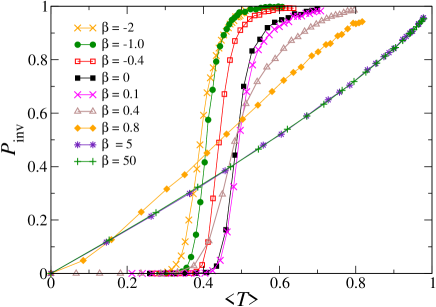
Figure 15: Probability of invasion as a function of the mean transmissibility for d-synergy in systems of linear size $L=31$. Different curves correspond to different values of $\beta$ as marked in the figure.

Appendix F Phase diagram for a simple model

The aim of this section is to present a simple model for evaluation of the phase diagram in $\alpha-\beta$ parameter space for both types of synergy in SIR process.

The phase transition from non-invasive to invasive SIR regime in heterogeneous systems with uncorrelated transmissibilities occurs when

$$\langle T\rangle=T_{c}~{},$$ (8)

where $T_{c}$ is a critical topology-dependent bond-percolation probability ($T_{c}=1/2$ for a square lattice) and $\langle T\rangle$ is the mean transmissibility Sander et al. (2002); PerezReche_JRSInterface2010 . For a synergistic SIR process, the transmissibilities are heterogeneous due to variable neighbourhood during infection (bond creating) process and correlated as it follows from our analysis of probability of invasion vs mean transmissibilities (see Sec. E). Such correlations make exact analytical treatment for synergistic SIR process hardly possible. However, if the correlations between transmissibilities are ignored then a simplified model for synergistic SIR process can be introduced and solved analytically for the boundaries in the phase diagram. The simplified assumptions of the model are the following:

• there are no correlations in transmissibilities;

• the neighbourhood of a r-d pair does not change over the infectious period of the donor;

• the probabilities of various neighbourhoods of a d-r do not depend on the rates $\alpha$ and $\beta$;

Under these assumptions, the analytical expressions for the phase boundaries reproducing qualitatively all the features found numerically can be derived and analysed.

F.1 d-synergy

We start analysis of the simplified model for synergistic SIR process on a square lattice (for concreteness) with the case of d-synergy. Let us consider an infected node (other than the initially infected host) which attempts to transmit infection (create a bond) to one of its susceptible neighbours during its infectious period $\tau=1$. This process can occur with different probability depending on the number of infected nodes linked to the infecting one (donor). Applying assumptions (i)-(ii) that transmissibilities are uncorrelated and a certain random neighbourhood does not change over the infectious period of the donor, we can calculate the mean transmissibility in the following way,

$$\langle T\rangle=\sum_{n=1}^{3}p_{n}T_{n}~{}.$$ (9)

Here $p_{n}$ is the probability that the donor is connected to $n$ ($n=1,2,3$ for square lattice) infected nodes and $n$-dependent transmissibility, $T_{n}$, for the d-r pair is

$$T_{n}=\left\{\begin{array}[]{ccc}1-e^{-\alpha-n\beta}{}{}{}&\text{if}&~{}~{}~{}\alpha+n\beta>0\\ 0{}{}{}&\text{if}&~{}~{}~{}\alpha+n\beta\leq 0~{}.\end{array}\right.$$ (10)

Different neighbourhoods of the d-r pair occur with probabilities $p_{n}$. Under assumption (iii), these probabilities do not depend on $\alpha$ and $\beta$ and given by the following expressions:

$$p_{1} =\frac{3p(1-p)^{2}}{1-(1-p)^{3}}~{},$$

$$p_{2} =\frac{3p^{2}(1-p)}{1-(1-p)^{3}}~{},$$

$$p_{3} =\frac{p^{3}}{1-(1-p)^{3}}~{},$$ (11)

where $p_{n}$ is the probability that the infecting node is linked to $n$ nodes given that it is linked at least to one out of three possible nodes and $p$ is the bond probability with $p=T_{c}$ at criticality. In Eq. (11), we used the assumption (i) that the bonds were created independently.

The locus of critical points can be found by solving Eq. (8),

$$T_{c}=\sum_{n=1}^{3}p_{n}(T_{c})T_{n}~{},$$ (12)

where $\langle T\rangle$ is given by Eqs. (9)-(11). Eq. (12) can be recast as $(\alpha>0)$,

$$\alpha=\begin{cases}-\ln(1-T_{c})+\ln\left(p_{1}(T_{c})e^{-\beta}+p_{2}(T_{c})e^{-2\beta}+p_{3}(T_{c})e^{-3\beta}\right)~{},~{}~{}~{}&\text{if}~{}~{}~{}\beta>-\alpha/3~{},\\ -\ln(1-T_{c}-p_{3}(T_{c}))+\ln\left(p_{1}(T_{c})e^{-\beta}+p_{2}(T_{c})e^{-2\beta}\right)~{},~{}~{}~{}&\text{if}~{}~{}~{}-\alpha/2<\beta\leq-\alpha/3~{},\\ -\ln(1-T_{c}-p_{3}(T_{c})-p_{2}(T_{c}))+\ln\left(p_{1}(T_{c})\right)-\beta~{},~{}~{}~{}&\text{if}~{}~{}~{}-\alpha<\beta\leq-\alpha/2~{},\end{cases}$$ (13)

and

$$\langle T\rangle=0~{},~{}~{}~{}\text{if}~{}~{}~{}\beta\leq-\alpha~{}.$$ (14)

i.e. the system is in non-invasive regime.

In the limiting case of small synergy, $|\beta|\ll 1$, the locus of critical points is given by a stright line,

$$\alpha\simeq-\ln(1-T_{c})-\langle n_{b}\rangle\beta=-\ln(1-T_{c})-\sum_{n=1}^{3}np_{n}\beta~{},$$ (15)

where $\langle n_{b}\rangle$ is the mean number of bonds attached to the donor given at least one bond atttached. For square lattice with $T_{c}=1/2$ and $p_{1}=p_{2}=3/7$, $p_{3}=1/7$, Eq. (15) gives

$$\alpha\simeq\ln(2)-12\beta/7~{}.$$ (16)

In the limiting case of strong interference, $\beta\to-\infty$, the phase boundary approaches the straight line asymptote, given by

$$\begin{split}\alpha&=-\ln(1-T_{c}-p_{3}(T_{c}))+\ln\left(p_{1}(T_{c})e^{-\beta}+p_{2}(T_{c})e^{-2\beta}\right)\\ &\simeq\ln\frac{p_{2}(T_{c})}{1-T_{c}-p_{3}(T_{c})}-2\beta=\ln(6/5)-2\beta~{},\end{split}$$ (17)

for square lattice.

The locus of critical points for d-synergy given by Eqs (13) and (14) is shown in Fig. 16 (dot-dashed line). The intersections of the critical line with the straight lines, $\beta=-\alpha/n$ ($n=1,2,3$), correspond to the changes in the regimes for the infection rates in Eqs. (13) and (14) and thus lead to appearance of the kinks (discontinuities in the derivatives) on the critical line. Within our approximations, the values of $p_{n}$ for square lattice are such that there is only one kink on the phase boundary for simple analytical model (corresponding to the crossing point of the phase boundary with $\beta=-\alpha/3$) and in the asymptotic regime, $\beta\to-\infty$, the phase boundary approaches linear asymptote, $\beta\simeq\beta^{\prime}_{0}-\alpha/2$ (with positive constant $\beta^{\prime}_{0}>0$).

Kinks are also expected on the phase boundary for the exact model. In order to check this, we have analysed the behaviour of the exact phase boundary obtained numerically around the point of intersection with the line $\beta=-\alpha/2$ (cf. Fig. 16). We have tested the presence of a kink by fitting a linear dependence $\beta=a+b\alpha$ to the data above and below the intersection. This procedure reveals a significant difference in the slope which takes values $b=-0.97$ and $b=-1.26$ above and below the intersection, respectively.

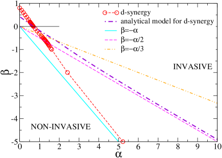
Figure 16: Locus of critical points for d-synergy within simple analytical model (dot-dashed line) compared with the exact numerical data (dashed line marked by circles). The intersections of the critical lines with straight lines, $\beta=-\alpha/n$, indicate the location of the kinks on the phase boundaries.

The locus of critical points in $\alpha-\beta$ parameter space derived within the simple analytical model (dot-dashed line in Fig. 16) is similar in shape to that obtained numerically (dashed line marked by the circles in Fig. 16). However, due to simplifying approximations (i)-(iii), the analytical model does not capture the asymptotic behaviour, $\beta\simeq\beta_{0}-\alpha$ (with positive constant $\beta_{0}>0$), obtained numerically for $\beta\to\-\infty$. This could be due to the fact that the actual probabilities $p_{n}$ (possibly depending on $\alpha$ and $\beta$ might be quite different from those used in the analytical model (see Eqs. (11)). The difference in gradients in the small-$\beta$ limit between analytically and numerically found phase boundaries can be due to similar reasons.

F.2 r-synergy

For $r$-synergy, the transmission of infection from a donor to a recipient can occur in the presence of different number of infected neighbours (in addition to the donor) of the recipient (for concreteness, we consider a square lattice for which $n=1,2,3$). Under assumptions (i) and (ii), the mean transmissibility for the d-r pair is,

$$\langle T\rangle=\sum_{n=0}^{3}q_{n}T_{n}~{},$$ (18)

where $q_{n}$ is the probability that the recipient has $n$ infected neighbours (in addition to the donor) and synergistic transmissibilities are given by Eq. (10) where $n=0,1,2,3$. The probabilities $q_{n}$ of different neighbourhoods of the recipient can be defined through the probability, $t$ (parameter of the model), that a nearest neighbour of the recipient host (different from the donor) is in the infected state,

$$q_{n}=C_{n}^{3}t^{n}(1-t)^{3-n}~{},$$ (19)

where we used the assumption about the independence of infection events for different neighbours of recipient. Given assumption (iii), from Eq. (8) written in the form,

$$T_{c}=\sum_{n=0}^{3}q_{n}T_{n}~{},$$ (20)

we can easily obtain the following equation for the locus of critical points:

$$\alpha=\begin{cases}-\ln(1-T_{c})+\ln\left(q_{0}(t)+q_{1}(t)e^{-\beta}+q_{2}(t)e^{-2\beta}+q_{3}(t)e^{-3\beta}\right)~{},&~{}~{}~{}\text{if}~{}~{}~{}\beta>-\alpha/3\\ -\ln(1-T_{c}-q_{3}(t))+\ln\left(q_{0}(t)+q_{1}(t)e^{-\beta}+q_{2}(t)e^{-2\beta}\right)~{},&~{}~{}~{}\text{if}~{}~{}~{}-\alpha/2<\beta\leq-\alpha/3\\ -\ln(1-T_{c}-q_{3}(t)-q_{2}(t))+\ln\left(q_{0}(t)+q_{1}(t)e^{-\beta}\right)~{},&~{}~{}~{}\text{if}~{}~{}~{}-\alpha<\beta\leq-\alpha/2\\ \alpha_{*}=\ln\frac{q_{0}(t)}{q_{0}(t)-T_{c}}~{},&~{}~{}~{}\text{if}~{}~{}~{}\beta\leq-\alpha~{}.\end{cases}$$ (21)

In the limit of large values of $\beta\to\infty$, the value of $\alpha$ approaches the asymptotic value $\alpha_{c}(\infty)$,

$$\alpha\to\alpha_{c}(\infty)=\ln\frac{q_{0}}{1-T_{c}}~{}.$$ (22)

The value of $\alpha_{c}(\infty)$ can be both positive and negative. We know from exact numerical analysis that $\alpha_{c}(\infty)>0$ ($\alpha_{c}(\infty)\simeq 0.2$) and thus we assume that

$$q_{0}=(1-t)^{3}>1-T_{c}~{},$$ (23)

i.e $t<1-(1-T_{c})^{1/3}$ ($t<7/8$, for square lattice).

In the limiting case of small values of $|\beta|\to 0$,

$$\begin{split}\alpha\to\alpha_{c}(\infty)=&-\ln(1-T_{c})-\sum_{1}^{3}nq_{n}\beta=\\ =&-\ln(1-T_{c})-\langle n\rangle\beta~{},\end{split}$$ (24)

where $\langle n\rangle$ is the mean value of infected neighbours (excluding the donor) of the recipient.

In the limiting case, $\beta\to-\infty$, the behaviour of the analytical critical line depends on the value of $t$. In particular, if $q_{0}=(1-t)^{3}>T_{c}$ then the critical line intersects the straight lines $\beta=-\alpha/n$ (resulting in kinks on the critical line) for all values of $n=1,2,3$ and becomes a vertical border at $\alpha=\alpha_{*}$ for $\beta\leq-\alpha_{*}$. Numerical data support such a scenario with the vertical border. The positions of both asymptotic value of $\alpha_{c}(\infty)$ and vertical border $\alpha_{*}$ vary with the value of $t$. In Fig. 17, the analytical critical lines are shown for two values of the node occupation probability $t$. For $t=0.047$, the behavior around small values of $\beta$ and position of the vertical border found numerically are reproduced quite well by the analytical model. However, the analytical curve strongly deviates from the numerical one for $\beta\gg 1$ and fails to reproduce the value of $\alpha_{c}(\infty)$. If we try to mimic the value of $\alpha_{c}(\infty)$ by tuning $t$ (see the curve for $t=0.152$), then the gradient at small $|\beta|$ and position of the vertical border are significantly off the numerical values. Such deviations area consequence of approximations (i)-(iii) used in the analytical model.

Overall, comparing the two types of synergy within the simple analytical model we can conclude that the main differences between them come from the presence of non-synergistic transmission events that are possible for r-synergy with any value of $\beta$ when the recipient is challenged by a single infected neighbour. Such transmission events with transmissibility $\propto 1-e^{-\alpha}$ are responsible for the appearance of the asymptotic value $\alpha_{c}(\infty)$ and vertical border $\alpha_{*}$ for r-synergy.

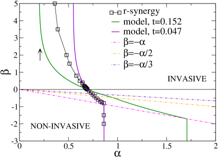
Figure 17: Locus of critical points for r-synergy within simple analytical model for two values of parameter $t$ (as indicated in the legend) compared with the exact numerical data. The intersections of the critical lines with the straight lines $\beta=-\alpha/n$ indicate the locations of the kinks on the phase boundaries.

References

- (1) R. Anderson and R. May, Phil. Trans. R. Soc. B 314, 533 (1986)
- (2) J. D. Murray, Mathematical Biology. Vol. I and II, 3rd ed. (Springer, 2002)
- (3) D. Centola, Science 329, 1194 (2010)
- (4) M. J. Keeling, Proc. R. Soc. B 266, 859 (1999)
- (5) P. Grassberger, Math. Biosci. 63, 157 (1983)
- (6) F. J. Pérez-Reche et al., J. Roy. Soc. Interface 7, 1083 (2010)
- (7) E. Kenah and J. Robins, Phys. Rev. E 76, 036113 (2007)
- (8) J. C. Miller, Phys. Rev. E 76, 010101 (2007)
- (9) S. C. Ferreira, M. L. Martins, and M. J. Vilela, Phys. Rev. E 65, 021907 (2002)
- (10) E. Ben-Jacob et al., Nature 368, 46 (1994)
- (11) A. D. M. Rayner, Mycologia 83, 48 (1991)
- (12) L. A. Liotta and E. C. Kohn, Nature 411, 375 (2001)
- (13) C. Castellano, S. Fortunato, and V. Loreto, Rev. Mod. Phys. 81, 591 (2009)
- (14) M. Henkel, H. Hinrichsen, and S. Lübeck, Non-Equilibrium Phase Transitions. Volume 1: Absorbing Phase Transitions (Springer, The Netherlands, 2009)
- (15) L. Pietronero, Phys. Rev. Lett. 55, 2025 (1985)
- (16) P. C. Hemmer and S. Hemmer, Phys. Rev. A 34, 3304 (1986)
- (17) S. Gubbins, C. A. Gilligan, and A. Kleczkowski, Theoretical Population Biology 57, 219 (2000)
- (18) M. J. Keeling et al., Science 294, 813 (2001)
- (19) P. S. Dodds and D. J. Watts, Phys. Rev. Lett. 92, 218701 (2004)
- (20) J. Shao, S. Havlin, and H. E. Stanley, Phys. Rev. Lett. 103, 018701 (2009)
- (21) M. Kitsak et al., Nature Phys., 6, 888 (2010)
- (22) L. M. Sander, et al., Math. Biosci. 180, 293 (2002)
- (23) D. J. Bailey, W. Otten, and C. A. Gilligan, New Phytol. 146, 535 (2000)
- (24) W. Otten, D. Bailey, and C. A. Gilligan, New Phytol. 163, 125 (2004)
- (25) S. Davis et al., Nature 454, 634 (2008)
- (26) R. Pastor-Satorras and A. Vespignani, Evolution and Structure of the Internet: A Statistical Physics Approach (Cambridge University Press, Cambridge, 2004)
- (27) D. M. Gordon, Ant encounters (Princeton University Press, Princeton, 2010)
- (28) D. Centola, V. M. Eguíluz, and M. W. Macy, Physica A 374, 449 (2007)
- (29) S. V. Fallert, J. J. Ludlam, and S. N. Taraskin, Phys. Rev. E 77, 051125 (2008)
- (30) See the special issue on “Complex Systems and Networks” edited by B. R. Jasny, L.M. Zahn, and E. Marshall [Science, 325, 405 (2009)].
- Pérez-Reche and Vives (2003) F. J. Pérez-Reche and E. Vives, Phys. Rev. B 67, 134421 (2003) NoStop
- Pérez-Reche et al. (2008) F. Pérez-Reche, L. Truskinovsky, and G. Zanzotto, Phys. Rev. Lett. 101, 230601 (2008) NoStop
- Stauffer and Aharony (1994) D. Stauffer and A. Aharony, Introduction to Percolation Theory, 2nd ed. (Taylor and Francis, 1994) NoStop
- Isichenko (1992) M. B. Isichenko, Rev. Mod. Phys. 64, 961 (1992) NoStop
- Ludwig (1975) D. Ludwig, Math. Biosc. 23, 33 (1975) NoStop
- Pellis et al. (2008) L. Pellis, N. M. Ferguson, and C. Fraser, Math. Biosc. 216, 63 (2008) NoStop
- Kuulasmaa (1982) K. Kuulasmaa, J. Appl. Prob. 19, 745 (1982) NoStop
- Cox and Durrett (1988) J. T. Cox and R. Durrett, Stochastic Processes And Their Applications 30, 171 (1988) NoStop
- Neri et al. (2011) F. M. Neri, F. J. Pérez-Reche, S. N. Taraskin, and C. A. Gilligan, J. Roy. Soc. Interface 8, 201 (2011) NoStop
- Handford et al. (2011) T. P. Handford, F. J. Pérez-Reche, S. N. Taraskin, L. d. F. Costa, M. Miazaki, F. M. Neri, and C. A. Gilligan, J. Roy. Soc. Interface 8, 423 (2011) NoStop
- Sander et al. (2002) L. M. Sander, C. P. Warren, I. M. Sokolov, C. Simon, and J. Koopman, Math. Biosci. 180, 293 (2002) NoStop