Laplacian Growth Without Surface Tension in Filtration Combustion: Analytical Pole Solution

Abstract

Filtration combustion is described by Laplacian growth without surface tension. These equations have elegant analytical solutions that replace the complex integro-differential motion equations by simple differential equations of pole motion in a complex plane. The main problem with such a solution is the existence of finite time singularities. To prevent such singularities, nonzero surface tension is usually used. However, nonzero surface tension does not exist in filtration combustion, and this destroys the analytical solutions. However, a more elegant approach exists for solving the problem. First, we can introduce a small amount of pole noise to the system. Second, for regularisation of the problem, we throw out all new poles that can produce a finite time singularity. It can be strictly proved that the asymptotic solution for such a system is a single finger. Moreover, the qualitative consideration demonstrates that a finger with $\frac{1}{2}$ of the channel width is statistically stable. Therefore, all properties of such a solution are exactly the same as those of the solution with nonzero surface tension under numerical noise. The solution of the ST problem without surface tension is similar to the solution for the equation of cellular flames in the case of the combustion of gas mixtures.

Keywords. Saffman - Taylor Problem, final time singularity, Laplacian Growth, Hele-Shaw cell, zero surface tension, Filtration Combustion, pole solution

1 Introduction

The problem of pattern formation is one of the most rapidly developing branches of nonlinear science today [1, 2, 3, 4, 5, 6, 7, 8, 9, 10, 11, 12, 13, 14, 15, 16, 17, 18].

The 2D Laplacian growth equation describes a wide range of physical problems, for example, filtration combustion in a porous medium, displacement of a cold liquid in a Hele-Shaw channel by the same liquid that is heated or of a hot gas in a Hele-Shaw channel by the same gas that is cooled, and solidification of a solid penetrating a liquid in a channel [2, 3, 4]. This equation has elegant analytical solutions ([30] and references inside). The subset of the solutions that have big physical sense can be written in the form of logarithmic poles (”Nevertheless, a considerable subclass of the purely logarithmic solutions is well defined for all positive times and describes a non-singular interface dynamics at zero surface tension” [30]). However, such an equation can lead to the appearance of final time singularities. To prevent these singularities and to regularise the problem, a term containing the surface tension is usually introduced into the equation describing Laplacian growth. Unfortunately, in the presence of such a surface tension term, obtaining an analytical solution in the form of poles becomes impossible. In addition, it is usually assumed that the surface tension explains the occurrence of an asymptotic solution in the form of a finger with half of the channel width. This asymptotic behaviour is also observed in experiments. In this paper, the mathematical mechanism of the regularisation is introduced. It makes it possible to avoid final time singularities, results in desirable asymptotic behaviour in the form of a finger with half of the channel width, and maintains the analytical solution in the form of poles. Maintenance of the analytical character of the solution is very important - it makes it possible to easily analyse 2D Laplacian growth solutions and to qualitatively or quantitatively explain the behaviour. The author sincerely hopes that this paper will play the same role for the 2D Laplacian growth equation as the paper [17] did for the theory of gaseous combustion of pre-mixed flames. The [17] analytical solution and its asymptotic behaviour have given a push to development of the theory of gaseous combustion of pre-mixed flames and have made it possible to qualitatively or quantitatively explain the behaviour of a front of pre-mixed flames [12, 13, 14, 15, 16, 18].

Matkowsky, Aldushin [2, 3, 4] considered planar, uniformly propagating combustion waves driven by the filtration of gas containing an oxidiser, which reacts with the combustible porous medium through which it moves. These waves were typically found to be unstable with respect to hydrodynamic perturbations for both forward (coflow) and reverse (counterflow) filtration combustion (FC), in which the direction of gas flow is the same as or opposite to the direction of propagation of the combustion wave, respectively.

The basic mechanism leading to instability is the reduction of the resistance to flow in the region of the combustion products due to an increase of the porosity in that region. Another destabilising effect in forward FC is the production of gaseous products in the reaction. In reverse FC, this effect is stabilising. In the case in which the planar front is unstable, an alternative mode of propagation in the form of a finger propagating with constant velocity was proposed. The finger region occupied by the combustion products is separated from the unburned region by a front in which chemical reactions and heat and mass transport occur.

In the paper of Matkowsky, Aldushin [2, 3, 4], it was shown that the finger solution of the combustion problem can be characterised as a solution of a Saffman-Taylor (ST) problem originally formulated to describe the displacement of one fluid by another having a smaller viscosity in a porous medium or in a Hele-Shaw configuration. The ST problem is known to possess a family of finger solutions, with each member characterised by its own velocity and each occupying a different fraction of the porous channel through which it propagates. The scalar field governing the evolution of the interface is a harmonic function. It is natural, then, to call the whole process $Laplacian$ $growth$.

The mathematical problem of Laplacian growth without surface tension exhibits a family of exact analytical solutions in terms of logarithmic poles in the complex plane.

The main problem with such a solution is existing finite time singularities. To prevent such singularities, nonzero surface tension usually is used ([5, 6, 7, 8, 9]). The surface tension also results in a well-defined asymptotic solution: only one finger with half of the channel width. In addition, the other terms can be used for regularisation (see [10, 11] and references therein).

The solution of the ST problem without surface tension is similar to the solution for the equation describing cellular flames in the case of combustion of gas mixtures [12, 13, 14, 15]. Indeed, in both cases, solutions can be transformed to the set of ordinary differential equations. This set describes the motion of poles in the complex plane. Applying nonzero surface tension to the ST problem destroys this elegant analytical solution.

It must be mentioned that the filtration combustion and the gaseous combustion in pre-mixed flames are features of different physics; the equation of 2D Laplacian growth and the equation describing the Mihelson-Sivashinsky feature use completely different mathematics. Moreover, whereas the equation for the Mihelson-Sivashinsky poles involves trigonometric functions, the equation for the 2D Laplacian growth poles involves logarithmic functions. The analogy here is not ”half-baked” but rather is deep. Indeed, the very different and complex integro-differential equations have a simple analytical solution in the form of poles. Moreover, even the behaviour of these poles is similar.

Another problem is the fact that surface tension may not be introduced for the mathematical problem considered by Saffman and Taylor involving filtration combustion in a porous medium [2, 3, 4]. Here, the zone of chemical reaction and diffusion of heat and mass shrinks to an interface separating the burned region from the unburned region. In all these problems, there is no pressure jump at the interface, so surface tension may not be introduced. Thus, the Saffman-Taylor model arises not only as the limiting case of zero surface tension in a problem in which surface tension enters the problem in a natural way but also in other situations in which the introduction of surface tension makes no sense. Another such problem is that of the solidification of a solid penetrating a liquid in a channel. It is reasonable to expect that the selection may be affected by introducing a perturbation other than surface tension that is relevant to the specific problem under consideration. For example, in the combustion problem, the effect of diffusion as a perturbation might be considered. Here, the effect of diffusion is similar to that of surface tension in the fluid displacement problem [2, 3, 4].

Therefore, we need to look for a solution without introducing surface tension using different methods for regularisation.

Criteria were proposed ([3] and [4]) to select the correct member of the family of solutions (one finger with half of the channel width) based on a consideration of the ST problem itself, rather than on modifications of the problem. A modification is obtained by adding surface tension to the model and then taking the limit of the vanishing surface tension.

It is nice that we know now the criteria for the correct asymptotic solution. Unfortunately, it is not clear from the papers why Laplacian growth without surface tension gives this asymptotic solution (one finger with half of the channel width) that satisfies the identified criteria (namely, which mathematical mechanism results in regularization of the problem). No proof exists in [3, 4] that the asymptotic solution must obey these criteria. These criteria are not derived theoretically from the motion equations, but are invented by authors from the knowledge of the experimental asymptotic solution.

In this paper, we introduce mathematical mechanism of regularization, which is not based on surface tension, and get the asymptotic solution. First of all, we can introduce a small amount of noise to the system. (The noise can be considered a pole flux from infinity.) Second, for regularization of the problem, we throw out all new poles that can produce a finite time singularity. It can be strictly proved that the asymptotic solution for such a system is a single finger. Moreover, the qualitative consideration demonstrates that a finger with $\frac{1}{2}$ of the channel width is statistically stable. Therefore, all properties of such a solution are exactly the same as for the solution with a nonzero surface tension under numerical noise.

The rest of the paper is organised as follows. Next, Section 2 describes asymptotic single Saffman-Taylor ”finger” formation without surface tension. Then we present arguments about Saffman-Taylor ”finger” formation with half of the channel size (Section 3). Finally (Section 4), we provide a summary and conclusions.

2 Asymptotic single Saffman-Taylor “finger” formation without surface tension

In the absence of surface tension, the effect of which is to stabilise the short-wavelength perturbations of the interface, the problem of 2D Laplacian growth is described as follows:

$$(\partial_{x}^{2}+\partial_{y}^{2})u=0\ .$$ (1)

$$u\mid_{\Gamma(t)}=0\ ,\partial_{n}u\mid_{\Sigma}=1\ .$$ (2)

$$v_{n}=\partial_{n}u\mid_{\Gamma(t)}\ .$$ (3)

Here, $u(x,y;t)$ is the scalar field mentioned, $\Gamma(t)$ is the moving interface, $\Sigma$ is a fixed external boundary, $\partial_{n}$ is a component of the gradient normal to the boundary (i.e. the normal derivative), and $v_{n}$ is a normal component of the velocity of the front.

Now, we introduce physical “no-flux” boundary conditions. This means no flux occurs across the lateral boundaries of the channel. This requires that the moving interface orthogonally intersects the walls of the channel. However, unlike the case of periodic boundary conditions, the end points at the two boundaries of the channel do not necessarily have the same vertical coordinate. Nevertheless, this can also be considered as a periodic problem in which the period equals twice the width of the channel. However, only half of this periodic strip should be considered as the physical channel, whereas the second half is its unphysical mirror image.

Then, we introduce a time-dependent conformal map $f$ from the lower half of a “mathematical” plane, $\xi\equiv\zeta+i\eta$, to the domain of the physical plane, $z\equiv x+iy$, where the Laplace equation 1 is defined as $\xi\stackrel{{\scriptstyle f}}{{\longrightarrow}}z$. We also require that $f(\xi,t)\approx\xi$ for $\xi\longrightarrow\zeta-i\infty$. Thus, the function $z=f(\zeta,t)$ describes the moving interface. From Eqs. (1), (2), and (3) for function $f(\xi,t)$ we obtain the $Laplacian$ $Growth$ $Equation$:

$$Im(\frac{\partial f(\xi,t)}{\partial\xi}\frac{\overline{\partial f(\xi,t)}}{\partial t})=1\mid_{\xi=\zeta-i0}\ ,f_{\xi}\mid_{\zeta-i\infty}=1\ .$$ (4)

Let us look for a solution of Eq. (4) in the following form:

$$f(\xi,t)=\lambda\xi-i{\tau(t)}-i\sum_{l=1}^{N}\alpha_{l}\log(e^{i{\xi}}-e^{i{\xi_{l}}(t)}),$$ (5)

$$z(\zeta,t)=f(\zeta,t)=\lambda\zeta-i{\tau(t)}-i\sum_{l=1}^{N}\alpha_{l}\log(e^{i{\zeta}}-e^{i{\xi_{l}}(t)}),$$ (6)

$$\alpha=\sum_{l=1}^{N}\alpha_{l}=1-\lambda,$$ (7)

where $\tau(t)$ is some real function of time, $\alpha_{l}$ is a complex constant, $\xi_{l}=\zeta_{l}+i\eta_{l}$ denotes the position of the pole with the number $l$, and $N$ is the number of poles.

For our “no-flux” boundary condition, we must add the condition that for every pole $\xi_{l}=\zeta_{l}+i\eta_{l}$ with $\alpha_{l}$ exists a pole $\xi_{l}=-\zeta_{l}+i\eta_{l}$ with $\overline{\alpha_{l}}$.

Therefore, we can conclude from this condition for pairs of poles and eq. (7) that $\lambda$ is a real constant.

We will prove below that the necessary condition for no finite time singularities for a pole solution is

$$-1<\lambda<1\ ,$$ (8)

Also, for the function $F(i{\xi},t)=if(\xi,t)$, for the “no-flux” boundary condition,

$$\overline{F(i{\xi},t)}=F(\overline{i\xi},t)$$ (9)

We want to prove that the final state will be only one finger if no finite time singularity appears during poles evolutions.

2.1 Asymptotic behaviour of the poles in the mathematical plane

This derivation is similar to [23], but we also consider “no-flux” boundary conditions here (in analogy with [24]).

The main purpose of this chapter is to investigate the asymptotic behaviour of the poles in the mathematical plane. We want to demonstrate that for time $t\mapsto\infty$, all poles go to the two boundary points for no-flux boundary conditions or to a single point for periodic boundary conditions.

The equation for the interface is

$$f(\xi,t)=\lambda\xi-i{\tau(t)}-i\sum_{l=1}^{N}\alpha_{l}\log(e^{i\xi}-e^{i{\xi_{l}}(t)}),$$

$$\sum_{l=1}^{N}\alpha_{l}=1-\lambda,-1<\lambda<1\ .$$ (10)

By substitution of Eq. (10) in the $Laplacian$ $Growth$ $Equation$,

$$Im(\frac{\partial f(\xi,t)}{\partial\xi}\frac{\overline{\partial f(\xi,t)}}{\partial t})=1\mid_{\xi=\zeta-i0}\ ,$$ (11)

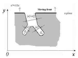
Figure 1: Geometrical interpretation of the complex constants of motion $\alpha_{k}^{\prime}=\frac{1}{2}\alpha_{k}$ and $\beta_{k}$; $k=1,...,N$.

we can find the equations of pole motion (Fig. 1):

$$\beta_{l}=\tau(t)+(1-\sum_{k=1}^{N}\overline{\alpha_{k}})\log\frac{1}{a_{l}}+\sum_{k=1}^{N}\overline{\alpha_{k}}\log(\frac{1}{a_{l}}-\overline{a_{k}})=const$$ (12)

and

$$\tau=t-\frac{1}{2}\sum_{k=1}^{N}\sum_{l=1}^{N}\overline{\alpha_{k}}\alpha_{l}\log(1-\overline{a_{k}}a_{l})+C_{0}\ ,$$ (13)

where $a_{l}=e^{i\xi_{l}}$ and $C_{0}$ is a constant.

From eqs. (12), we can find

$$(1-\lambda)\tau-\sum_{l=1}^{N}\alpha_{l}\log a_{l}+$$

$$\sum_{k=1}^{N}\sum_{l=1}^{N}\overline{\alpha_{k}}\alpha_{l}\log(1-\overline{a_{k}}a_{l})=const\ .$$ (14)

From eqs. (13) and (14), we can obtain

$$Im(\sum_{l=1}^{N}\alpha_{l}\log a_{l})=const$$ (15)

and

$$t=(\frac{1+\lambda}{2})\tau+\frac{1}{2}Re(\sum_{l=1}^{N}\alpha_{l}\log a_{l})+C_{1}/2\ ,$$ (16)

where $C_{1}$ and $\alpha_{l}$ are constants, $\xi_{l}(t)$ is the position of the poles, and $a_{l}=e^{i{\xi_{l}}(t)}$.

In Appendix A, we will prove from eq.(13) that $\tau\mapsto\infty$ if $t\mapsto\infty$ and if no finite time singularity exists.

The equations of pole motion that follow from eqs. (12) are as follows:

$$\tau+i\overline{\xi_{k}}+\sum_{l}\alpha_{l}\log(1-e^{i(\xi_{l}-\overline{\xi_{k}})})=const,$$ (17)

or in a different form:

$$\zeta_{k}+\sum_{l}(\alpha_{l}^{\prime\prime}\log\mid 1-e^{i(\xi_{l}-\overline{\xi_{k}})}\mid+$$

$$\alpha_{l}^{\prime}\arg(1-e^{i(\xi_{l}-\overline{\xi_{k}})}))=const,$$ (18)

$${\tau}+\eta_{k}+\sum_{l}(\alpha_{l}^{\prime}\log\mid 1-e^{i(\xi_{l}-\overline{\xi_{k}})}\mid-$$

$$\alpha_{l}^{\prime\prime}\arg(1-e^{i(\xi_{l}-\overline{\xi_{k}})}))=const,$$ (19)

where

$$\xi_{l}=\zeta_{l}+i\eta_{l},\eta_{l}>0\ .$$ (20)

$$\alpha_{l}=\alpha_{l}^{\prime}+i\alpha_{l}^{\prime\prime}\ .$$ (21)

Let us transform

$$\arg(1-e^{i(\xi_{l}-\overline{\xi_{k}}})=$$

$$\arg([1-e^{i(\zeta_{l}-\zeta_{k})}e^{-(\eta_{l}+\eta_{k})}])=$$

$$\arg[1-a_{lk}e^{i\varphi_{lk}}]$$ (22)

$$\varphi_{lk}=\zeta_{l}-\zeta_{k},a_{lk}=e^{-(\eta_{l}+\eta_{k})}$$ (23)

$\arg[1-a_{lk}e^{i\varphi_{lk}}]$ is a single-valued function of $\varphi_{lk}$, i.e.,

$$-\frac{\pi}{2}\leq\arg[1-a_{lk}e^{i\varphi_{lk}}]\leq\frac{\pi}{2}\ .$$ (24)

We multiply eq. (19) by $\alpha_{k}^{\prime\prime}$ and eq. (18) by $\alpha_{k}^{\prime}$, and taking the difference, we obtain the following equation:

$$\alpha_{k}^{\prime}\zeta_{k}-\alpha_{k}^{\prime\prime}\tau+$$

$$\sum_{l\neq k}((\alpha_{l}^{\prime\prime}\alpha_{k}^{\prime}-\alpha_{k}^{\prime\prime}\alpha_{l}^{\prime})\log\mid 1-e^{i(\xi_{l}-\overline{\xi_{k}})}\mid+$$

$$(\alpha_{l}^{\prime}\alpha_{k}^{\prime}+\alpha_{l}^{\prime\prime}\alpha_{k}^{\prime\prime})\arg(1-e^{i(\xi_{l}-\overline{\xi_{k}})}))=const.$$ (25)

We want to investigate the asymptotic behaviour of poles $\tau\mapsto\infty$.

We have the divergent terms $\alpha_{k}^{\prime\prime}\tau$ in this equation. From eq. (25 ), only the term $\log\mid 1-e^{i(\xi_{l}-\overline{\xi_{k}})}\mid$ can eliminate this divergence. The necessary condition for this to occur is $\eta_{k}\mapsto 0$ for $\tau\mapsto\infty,1\leq k\leq N$.

We may assume that for $t\mapsto\infty$, $N^{\prime}$ groups of poles exist (${N^{\prime}\leq N}$) ($\varphi_{lk}\mapsto 0$ for all members of a group). The $N^{\prime}$ is currently arbitrary and can even be equal to $N$. $N_{l}$ is the number of poles in each group, $1\leq l\leq N^{\prime}$.

For each group, by summation of eqs. (25) over all group poles, we obtain

$$\alpha_{k}^{gr\prime}\zeta_{k}^{gr}-\alpha_{k}^{gr\prime\prime}\tau+$$

$$\sum_{l\neq k}((\alpha_{l}^{gr\prime\prime}\alpha_{k}^{gr\prime}-\alpha_{k}^{gr\prime\prime}\alpha_{l}^{gr\prime})\log\mid 1-e^{i(\xi_{l}^{gr}-\overline{\xi_{k}^{gr}})}\mid+$$

$$(\alpha_{l}^{gr\prime}\alpha_{k}^{gr\prime}+\alpha_{l}^{gr\prime\prime}\alpha_{k}^{gr\prime\prime})\arg(1-e^{i(\xi_{l}^{gr}-\overline{\xi_{k}^{gr}})}))=const,$$ (26)

where

$$\alpha_{l}^{gr\prime\prime}=\sum_{k}^{N_{l}}\alpha_{k}^{\prime\prime}\ ,$$ (27)

$$\alpha_{l}^{gr\prime}=\sum_{k}^{N_{l}}\alpha_{k}^{\prime}\ .$$ (28)

We have no merging between defined groups for large $\tau$, so we investigate the motion of poles with this assumption:

$$\mid\zeta_{l}^{gr}-\zeta_{k}^{gr}\mid\gg\eta_{l}^{gr}+\eta_{k}^{gr},1\leq l,k\leq N\ .$$ (29)

For $l\neq k$, $\eta_{k}^{gr}\mapsto 0$, and $\varphi_{lk}^{gr}=\zeta_{l}^{gr}-\zeta_{k}^{gr}$, we obtain

$$\log\mid 1-e^{i(\xi_{l}^{gr}-\overline{\xi_{k}^{gr}})}\mid\approx\log\mid 1-e^{i(\zeta_{l}^{gr}-\zeta_{k}^{gr})}\mid=$$

$$\log 2+\frac{1}{2}\log\sin^{2}\frac{\varphi_{lk}^{gr}}{2}$$ (30)

and

$$\arg(1-e^{i(\xi_{l}^{gr}-\overline{\xi_{k}^{gr}})})\approx\arg(1-e^{i(\zeta_{l}^{gr}-\zeta_{k}^{gr})})=$$

$$\frac{\varphi_{lk}^{gr}}{2}+\pi n-\frac{\pi}{2}\ .$$ (31)

We choose $n$ in Eq.(31) so that Eq.(24) is correct. Substituting these results into eqs. (26), we obtain

$$C_{k}={\alpha^{gr\prime}{\zeta_{k}^{gr}}}-\alpha_{k}^{gr\prime\prime}\tau+$$

$$\sum_{l\neq k}[({\alpha_{l}^{gr\prime\prime}\alpha_{k}^{gr\prime}}-{\alpha_{k}^{gr\prime\prime}\alpha_{l}^{gr\prime}})\log\mid\sin\frac{\varphi_{lk}^{gr}}{2}\mid$$

$$+(\alpha_{l}^{gr\prime}\alpha_{k}^{gr\prime}+{\alpha_{l}^{gr\prime\prime}\alpha_{k}^{gr\prime\prime})}\frac{\varphi_{lk}^{gr}}{2}].$$ (32)

2.2 Theorem about coalescence of the poles

From eqs. (32), we can conclude the following:

(i) By summation of eqs. (32) (or exactly from eq. (15)), we obtain

$$\sum_{k}\alpha_{k}^{gr\prime}{\zeta_{k}^{gr}}=const\ .$$ (33)

(ii) For $\mid{\varphi}_{lk}^{gr}\mid\mapsto 0,2\pi$, we obtain $\log\mid\sin\frac{\varphi_{lk}^{gr}}{2}\mid\mapsto\infty$, meaning that the poles can not pass each other;

(iii) From (ii), we conclude that $0<\mid\varphi_{lk}^{gr}\mid<2\pi$;

(iv) From (i) and (iii), $\zeta_{k}^{gr}\mapsto\infty$ is impossible;

(v) In eq.(32), we must compensate for the second divergent term. From (iv) and (iii), we can do this only if $\alpha_{l}^{gr\prime\prime}=\sum_{k}^{N_{l}}\alpha_{k}^{\prime\prime}=0$ for all $l$.

Therefore, from eq. (32), we obtain

$$\sum_{k}^{N_{l}}\alpha_{k}^{\prime\prime}=0\ ,$$ (34)

$$\dot{\varphi_{lk}^{gr}}=0\ ,$$ (35)

$${\varphi_{lk}^{gr}}\neq 0\ ,$$ (36)

$$\dot{\zeta_{k}^{gr}}=0\ .$$ (37)

For the asymptotic motion of poles in group $N_{m}$, we obtain the following from eqs. (34), (35), (36), and (37), taking the leading terms in eqs. (16) and (17):

$$\tau=\frac{2}{\lambda+1}t\ ,$$ (38)

$$0=\dot{\tau}+\sum_{l}^{N_{m}}\alpha_{l}\frac{\dot{\eta_{k}}+\dot{\eta_{l}}+i(\dot{\zeta_{k}}-\dot{\zeta_{l}})}{\eta_{k}+\eta_{l}+i(\zeta_{k}-\zeta_{l})}\ .$$ (39)

The solution to these equations is

$$\eta_{k}=\eta_{k}^{0}e^{-\frac{1}{\alpha_{m}^{gr\prime}}\frac{2}{1+\lambda}t}\ ,$$ (40)

$$\varphi_{lk}={\varphi_{lk}}^{0}e^{-\frac{1}{\alpha_{m}^{gr\prime}}\frac{2}{1+\lambda}t}\ ,$$ (41)

$$\dot{\zeta_{k}}=0\ .$$ (42)

Therefore, we may conclude that to eliminate the divergent term, we need

$$\alpha_{l}^{gr\prime\prime}=\sum_{k}^{N_{l}}\alpha_{k}^{\prime\prime}=0,$$ (43)

$$\alpha_{l}^{gr\prime}(1+\lambda)>0$$ (44)

for all $l$.

2.3 The final result

With the periodic boundary condition, eq.(43) is correct for all poles, so we obtain $N^{\prime}=1$, $m=1$ and $N_{m}=N$.

Therefore the unique solution is

$$\eta_{k}=\eta_{k}^{0}e^{-{2\over(1-\lambda^{2})}t}\ ,$$ (45)

$$\varphi_{lk}={\varphi_{lk}}^{0}e^{-{2\over(1-\lambda^{2})}t}\ ,$$ (46)

$$\dot{\zeta_{k}}=0\ .$$ (47)

$$1-\lambda^{2}>0$$ (48)

With the no-flux boundary condition, we have a pair of poles whose condition in eq. (43) is correct, so all these pairs must merge. Because of the symmetry of the problem, these poles can merge only on the boundaries of the channel $\zeta=0,\pm\pi$. Therefore, we obtain two groups of the poles on boundaries. $N^{\prime}=2$, $m=1,2$, $N_{1}+N_{2}=N$, and $\alpha_{1}^{gr\prime}+\alpha_{2}^{gr\prime}=1-\lambda$. (In principle, it is possible for some degenerate case of $\alpha_{l}^{gr\prime}$ values that eq. (43) would be correct for some different groups of poles. However, this is a very improbable, rare case.)

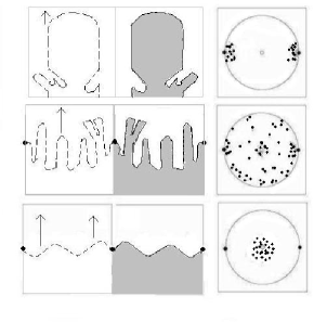
Figure 2: Three consecutive stages of fingering in the Hele-Shaw cell: initial (left), intermediate (center), and asymptotic (right). The physical plane $z$ is shown in the upper pictures, while the lower pictures depict a distribution of moving poles $a_{k}(t)$ in the unit circle $|\omega|<1$ on the mathematical plane $\omega$. The open circle indicates the repeller, $\omega=0$, while the solid circle indicates the attractor, $\omega=1$, of poles whose dynamics is given by (12-13).

Consequently, we obtain the solution (on two boundaries of the channel Fig. 2):

$$\eta_{k}^{(1)}=\eta_{k}^{(1),0}e^{-\frac{1}{\alpha_{1}^{gr\prime}}\frac{2}{1+\lambda}t}\ ,$$ (49)

$$\varphi_{lk}^{(1)}={\varphi_{lk}}^{(1),0}e^{-\frac{1}{\alpha_{1}^{gr\prime}}\frac{2}{1+\lambda}t}\ ,$$ (50)

$${\zeta_{k}^{(1)}}=0\ ;$$ (51)

$$\eta_{k}^{(2)}=\eta_{k}^{(2),0}e^{-\frac{1}{\alpha_{2}^{gr\prime}}\frac{2}{1+\lambda}t}\ ,$$ (52)

$$\varphi_{lk}^{(2)}={\varphi_{lk}}^{(2),0}e^{-\frac{1}{\alpha_{2}^{gr\prime}}\frac{2}{1+\lambda}t}\ ,$$ (53)

$${\zeta_{k}^{(2)}}=\pm\pi\ ;$$ (54)

$$\alpha_{1}^{gr\prime}(1+\lambda)>0,$$ (55)

$$\alpha_{2}^{gr\prime}(1+\lambda)>0.$$ (56)

By summation of eqs. (55) and (55) and using eq. 7, we obtain

$$(1-\lambda)(1+\lambda)=1-\lambda^{2}>0.$$ (57)

This immediately gives us the formerly formulated condition (8) for $\lambda$.

$\frac{\lambda+1}{2}=1-\frac{\alpha}{2}$ has an explicit physical sense. It is the portion of the channel occupied by the moving liquid. We see that for no finite time singularity and for $t\mapsto\infty$, we obtain one finger with width $\frac{\lambda+1}{2}$.

3 Saffman-Taylor ”finger” formation with half of the channel size

The case of Laplacian growth in the channel without surface tension was considered in detail by Mineev-Weinstein and Dawson [19]. In this case, the problem has an elegant analytical solution. Moreover, they assumed that all major effects in the case with vanishingly small surface tension may also occur without surface tension. This would make it possible to apply the powerful analytical methods developed for the no surface tension case to the vanishingly small surface tension case . However, without additional assumptions, this hypothesis may not be accepted.

The first objection is related to finite time singularities for some initial conditions. Actually, for overcoming this difficulty, a regular item with surface tension was introduced. This surface tension item results in loss of the analytical solution. However, regularisation may be carried out much more simply - simply by rejecting the initial conditions that result in these singularities.

The second objection is given in work by Siegel and Tanveer [20]. There, it is shown that in numerical simulations (supported by some semi-analytical calculations with appearance ”daughter singularity”) in a case with any (even vanishingly small) surface tension, any initial thickness ”finger” extends up to $\frac{1}{2}$ the width of the channel during finite time, witch does not depend on value of small surface tension. The analytical solution in a case without surface tension results in a constant thickness of the “finger” equal to its initial size, which may be arbitrary. Siegel and Tanveer, however, did not take into account the simple fact that numerical noise introduces small perturbation to the initial condition or even during “finger” growth, which is equivalent to the remote poles, and with respect to this perturbation, the analytical solution with a constant “finger” is unstable.

It was shown by Mineev-Weinstein [21] that similar pole perturbations for some initial conditions, can be extended to the Siegel and Tanveer solutions. This positive aspect of the paper [21] was mentioned by Sarkissian and Levine in their Comment [22] and in Reply of Mineev-Weinstein [28]. In summary, it is possible to determine that to identify the results with and without surface tension, it is necessary to introduce a permanent source of the new remote poles: the source may be either external noise or an infinite number of poles in an initial condition. Which of these methods is preferred is still an open question.

Of course, this additional noise will insert new poles resulting in solutions, which are different from Siegel and Tanveer solution [22]. However, these solutions appear as a result of the noise both without surface tension and with surface tension. Thus, introducing the noise erases difference between equation with surface tension and without surface tension.

In the case of flame front propagation, it was shown [12, 13, 14, 15, 16] that external noise is necessary for an explanation of the flame front velocity increase with the size of the system: using an infinite number of poles in an initial condition cannot give this result. It is interesting to know what the situation is in the channel Laplacian growth. One of the main results of Laplacian growth in the channel with a small surface tension is Saffman-Taylor “finger” formation with a thickness equal to $\frac{1}{2}$ the thickness of the channel. To use the analytical result obtained for zero surface tension, it is necessary to prove that formation of the “finger” also takes place without surface tension.

In our teamwork with Mineev-Weinstein [23], it was shown that for a finite number of poles at almost all allowed (in the sense of not approaching finite time singularities) initial conditions, except for a small number of degenerate initial conditions, there is an asymptotic solution involving a “finger” with any possible thickness. Note that the solutions and asymptotic behaviour found in [23] for a finite number of poles are an idealisation but have a real sense for any finite intervals of time between the appearance of the new poles introduced into the system by external noise or connected to an entrance to the system of remote poles of an initial condition, including an infinite number of such poles. The theorem proved in [23] may again be applied for this final set of new and old poles and again yields asymptotic behaviour in the form of a “finger”, but the thickness is different. Thus, introduction of a source of new poles results only in possible drift of the thickness of the final “finger” but does not change the type of solution.

It should be mentioned that instead of periodic boundary conditions, much more realistic “no flux” boundary conditions may be introduced [24]. (This paper repeats the result for single finger asymptotic behaviour already proved formerly in the papers [23]. See also reference 14 in [21] and reference 20 (and correspondent text) in [23]). This result forbids a stream through a wall, which inserts additional, probably useful restrictions on the positions, number, and parameters of new and old poles (explaining, for example, why the sum of all complex parameters $\alpha_{i}$ for poles gives the real value $\alpha$ for the pole solution (5) in [21]). However, this does not have an influence on the correctness and applicability of the results and methods proved in [23]. No new qualitative results appear as a result of introducing “no flux” boundary conditions. For example, one finger asymptotic behaviour is correct for the both cases.

Mineev-Weinstein [21] tries to give proof that steady asymptotic behaviour for Laplacian growth in a channel with zero surface tension is a single “finger” with a thickness equal to $\frac{1}{2}$ the thickness of the channel, which is unequivocally erroneous. Indeed, the method in [21] proves and demonstrates the instability of a “finger” with a thickness distinct from $\frac{1}{2}$ with respect to introducing new remote poles. However, the instability of a “finger” with a thickness equal to $\frac{1}{2}$ may be proved and demonstrated by the same method.

Such instability is justified explicitly in Comments of Casademunt, Magdaleno and Almgren [25, 26]. Casademunt and Magdaleno write, that perturbation of a finger solution considered by Mineev-Weinstein in [21] (precisely, perturbation of the $\lambda\zeta$ term in the conformal representation $z(\zeta,t)$ ), represents a special case of more general perturbation:

$$\lambda\zeta\approx(\lambda-\lambda_{0})\zeta-i\sum_{k=1}^{N}\delta_{k}\log(e^{i{\zeta}}-\epsilon_{k}),$$ (58)

where $\epsilon_{k}$ is small, and $\sum_{k=1}^{N}\delta_{k}=\lambda_{0}$ .

Perturbation considered by Mineev-Weinstein in [21] corresponds to the case $\lambda=\lambda_{0}$:

$$\lambda\zeta\approx-i\sum_{k=1}^{N}\delta_{k}\log(e^{i{\zeta}}-\epsilon_{k}),$$ (59)

The finger with the thickness of $\frac{1}{2}$ corresponds to the case $\lambda=0$. Such finger will be stable with respect to perturbation of Mineev-Weinstein in [21], but is unstable to more common perturbation of Casademunt and Magdaleno in [25]. It contradicts with the statment of [21], that the solution in the form of the finger $\frac{1}{2}$ is stable and, corespondently, is asymtotic for all other unstable solutions. The answer to this objection is done by Mineev-Weinstein in Reply [27]. He demonstrate, that perturbation of Casademunt and Magdaleno can be easily transformed to the perturbation of Mineev-Weinstein by adding a pole in zero. From this, Mineev-Weinstein makes two conclusions:

1) Perturbation of Casademunt and Magdaleno is unstable. Really, for the proof of instability, it is enough to prove instability with respect to at least one perturbation. Such perturbation is the additive pole. As perturbation of Casademunt and Magdaleno is unstable and can be transformed to perturbation odf Mineev-Weinstein , Mineev-Weinstein concludes, that it has no sense to used perturbation of Casademunt and Magdaleno.

2)Perturbations of Casademunt and Magdaleno is only ”small” subset of perturbations of Mineev-Weinstein for a case of an additive pole in zero. Mineev-Weinstein concludes, that perturbations of Casademunt and Magdaleno are ”much rare”, than perturbations of Mineev-Weinstein . Therefore, it has no sense to used perturbation of Casademunt and Magdaleno. The first objection paradoxically works against arguments of Mineev-Weinstein . Indeed, if for the proof of instability it is enough to show instability with respect to at least one perturbation . It means that instability of the finger $\frac{1}{2}$ with respect to perturbation of Casademunt and Magdaleno is quite enough to proof instability of the finger $\frac{1}{2}$. Accordingly, the finger $\frac{1}{2}$ cannot be an asymptotics. The second objection contains a simple mathematical error. Really, for the set theory, the subset can be equal to the set. For example, squares of the natural numbers are only a subset of the natural numbers. However, between both sets there is an obvious one-to-one correspondence. For the current case, for each perturbation of Mineev-Weinstein resulting in the finger $\frac{1}{2}$:

$$\lambda\zeta\approx-i\sum_{k=1}^{N}\delta_{k}\log(e^{i{\zeta}}-\epsilon_{k}),$$ (60)

is possible to find the correspondent perturbation of Casademunt and Magdaleno:

$$0\zeta\approx(0-(-\lambda))\zeta-i\sum_{k=1}^{N}(-\delta_{k})\log(e^{i{\zeta}}-\epsilon_{k}),$$ (61)

returning the thickness of the finger $\frac{1}{2}$ to the initial value. Moreover, in our teamwork [23], it is shown that for a finite number of poles, any thickness “finger” is possible as an asymptotic solution.However, some factor exists which can break describe above one-to-one correspondence between perturbation of Mineev-Weinstein resulting in the finger $\frac{1}{2}$ and perturbation of Casademunt and Magdaleno returning the thickness of the finger $\frac{1}{2}$ to the initial value. Indeed, some of these perturbation result in finite time singularities, not asymptotic finger. If these singularities appear more frequently for perturbation of Mineev-Weinstein then perturbation of Casademunt and Magdaleno we can get exlusive role of the finger $\frac{1}{2}$. Exactly this situation appears in our consideration below (see Fig. 3).

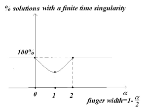
Figure 3: The width of the finger is equal to $1-\frac{\alpha}{2}$ (The channel width is assumed to be equal to 1). The graph for the current $\alpha$ gives the percent of all possible solutions resulting in a finite time singularity. The maximum value is equal to 100 percent and corresponds to ${\alpha\leq 0}$ or ${\alpha\geq 2}$. The minimum is located at the middle point $\alpha=1$ between $\alpha=0$ (finger width of 1) and $\alpha=2$ (finger width of 0). Therefore, at the minimum, the finger width is $\frac{1}{2}$.

This does not mean, however, that the privileged role of a “finger” no surface tension; it only means that the proof is not given in [21]. Let us try to give the correct arguments here. The general pole solution (5) in work [21] is characterized by the real parameter $\alpha$ being the sum of the complex parameters $\alpha_{i}$ for poles. The thickness of the asymptotic finger is a simple function of $\alpha$: (Thickness = $1-\frac{\alpha}{2}$). The value ($\alpha=1$) corresponds to a thickness of $\frac{1}{2}$. As far as possible, the thickness of the “finger” is between 0 and 1, and the possible $\alpha$ value is in an interval between 0 and 2: ($0<\alpha<2$). The value $\alpha=1$ corresponding to the finger width $\frac{1}{2}$ is exactly in the middle of this interval. What happens to the quite possible initial pole conditions with $\alpha$ outside of the limits from 0 to 2? They are “not allowed” because of the already identified finite time singularities [23]. Also, a part of the solutions inside the interval $0<\alpha<2$ results in similar finite time singularities.

Finding exact sufficient and necessary conditions when defining the initial pole condition as “not allowed”, i.e., singular, is still an open problem. How are these “not allowed” initial pole conditions (to be precise, their percentage from the full number of possible initial pole conditions corresponding to the given real value $\alpha$) distributed inside of the interval $0<\alpha<2$?

From reasons of continuity and symmetry with respect to $\alpha=1$ (Fig. 3), it is possible to conclude that this distribution has a minimum at point $\alpha=1$ (thickness $\frac{1}{2}$!), the value that is the most remote from both borders of the interval $0<\alpha<2$, and that the distribution increases to the borders $\alpha=2$ and 0, reaching 100 percent for all pole solutions outside of these borders, i.e., the thickness $\frac{1}{2}$ is the most probable because for this thickness value, the minimal percent of initial conditions potentially capable of producing such a thickness value is “not allowed”, i.e., results in singularities.

A source of new poles results in drift of the finger thickness, but this thickness drift is close to the most probable and average size equal to $\frac{1}{2}$. A similar result is obtained in the case of a Saffman-Taylor “finger” with vanishingly small surface tension and with some external noise, which was one of the goals of the paper.

Let’s formulate shortly our conclusion. For detailed consideration of the solution stability is necessary to consider explicitly the noise which can be presented as a stream of poles from zero. If such noise is not presented in computer calculations, the numerical noise (related to terminating accuracy of evaluations) plays a part of the explicit noise . In the presence of such noise, it is possible to consider not asymptotic, but a stochastic stability of the finger $\frac{1}{2}$. Such stability arises from the regularization of the solution by rejection of poles from the noise, which are able to lead to finite time singularities. During such rejection for the finger $\frac{1}{2}$, the probabilities of appearance of poles, decreasing or increasing finger’s thickness, are identical. For a finger with a thickness in distinct from $\frac{1}{2}$, the probability of appearance of poles, shifting its thickness to $\frac{1}{2}$ is more probable.

It is interesting (from this point of view) to consider outcomes of Kessler and Levine [29]. In the paper, the case of asymmetric surface tension converging to zero is considered. It is demonstrated, that for very small surface tension, the asymptote is not the finger $\frac{1}{2}$, but random noise. The Kessler and Levine conclude about senselessness of the analysis of the asymptotic solution as the finger $\frac{1}{2}$ for a case of the surface tension converging to zero. However authors make the same error, as Siegel and Tanveer in [20]. It is necessary to consider explicitly, not only the surface tension, but also the noise (at least, small numerical noise). For the small surface tension, the big noise can lead to appearance of a new singularities before or immediately after the disappearance of previous singularity, smoothed by the small surface tension. It leads to the random solution described in the paper [31]. I.e., for forming the asymptotic finger $\frac{1}{2}$, it is necessary not only a small surface tension, but also small noise, which is not considered in [29].

It should be mentioned that these formulated arguments are only qualitative and that a strict proof is also necessary. The first step to this direction was made in [31, 32]. Unfortunately, analysis of asymptotic solution for Laplacian growth was made in [31] in absence of the noise. It is physically unsensible. For asymptotic solution with noise and regularization (by shift out unphysical and singular solutions), results of [31] rather confirm the conclusions of this paper and can be the first step for mathematical formalization of these conclusions.

4 Conclusions

The analytical pole solution for Laplacian growth sometimes yields finite time singularities. However, an elegant solution of this problem exists. First, we introduce a small amount of noise to system. This noise can be considered as a pole flux from infinity. Second, for regularisation of the problem, we throw out all new poles that can give a finite time singularity. It can be strictly proved that the asymptotic solution for such a system is a single finger. Moreover, the qualitative consideration demonstrates that the finger equal to $\frac{1}{2}$ of the channel width is statistically stable. Therefore, all properties of such a solution are exactly the same as those of the solution with a nonzero surface tension under numerical noise.

Surprisingly, the flame front propagation problem (in spite of exhibiting absolutely different physics and mathematical equations for motion) also has analytical pole solutions and demonstrates the same qualitative behaviour as these solutions [12, 13, 14, 15, 16].

5 Appendix A

We need to prove that $\tau\mapsto\infty$ if $t\mapsto\infty$ and if no finite time singularity exists. The formula for $\tau$ is as follows:

$$\tau=t+[-\frac{1}{2}\sum_{k=1}^{N}\sum_{l=1}^{N}\overline{\alpha_{k}}\alpha_{l}\log(1-\overline{a_{k}}a_{l})]+C_{0}\ ,$$ (62)

where $\mid a_{l}\mid<1$ for all $l$.

Let us prove that the second term in this formula is greater than zero:

$$-\frac{1}{2}\sum_{k=1}^{N}\sum_{l=1}^{N}\overline{\alpha_{k}}\alpha_{l}\log(1-\overline{a_{k}}a_{l})=$$

$$-\frac{1}{2}\sum_{k=1}^{N}\sum_{l=1}^{N}\overline{\alpha_{k}}\alpha_{l}\sum_{n=1}^{\infty}(-\frac{(\overline{a_{k}}a_{l})^{n}}{n})=$$

$$\frac{1}{2}\sum_{n=1}^{\infty}\frac{1}{n}(\sum_{k=1}^{N}\overline{\alpha_{k}}(\overline{a_{k}})^{n})(\sum_{l=1}^{N}\alpha_{l}(a_{l})^{n})=$$

$$\frac{1}{2}\sum_{n=1}^{\infty}\frac{1}{n}\overline{(\sum_{l=1}^{N}\alpha_{l}(a_{l})^{n})}(\sum_{l=1}^{N}\alpha_{l}(a_{l})^{n})>0$$ (63)

Therefore, the second term in eq. (62) always greater than zero, and consequently, $\tau\mapsto\infty$ if $t\mapsto\infty$ for no finite time singularity.

Acknowledgments We would like to thank Mark Mineev-Weinstein for his many fruitful ideas, which were very useful for creating the paper.

References

- [1] P. Pelce, Dynamics of Curved Fronts, Academic Press, Boston (1988)
- [2] A.P. Aldushin, B.J. Matkowsky, Combust. Sci. Tech. 133 (1998) 293-341.
- [3] A.P. Aldushin, B.J. Matkowsky, Appl. Math. Lett. 11 (1998) 57-62.
- [4] A.P. Aldushin, B.J. Matkowsky, Phys. Fluids 11 (1999) 1287-1296.
- [5] S.J. Chapman, Eur J. Appl. Math. 10 (1999) 513-534.
- [6] R. Combescot, T. Dombre, V. Hakim, Y. Pomeau, Phys. Rev. Lett. 56 (1986) 2036-2039.
- [7] R. Combescot, V. Hakim, T. Dombre, Y. Pomeau, A. Pumir, Phys. Rev. A 37 (1988) 1270-1283.
- [8] D.C. Hong, J.S. Langer, Phys. Rev. Lett. 56 (1986) 2032-2035.
- [9] B.I. Shraiman, Phys. Rev. Lett. 56 (1986) 2028-2031.
- [10] S.J. Chapman, J.R. King, J. Eng. Math. 46 (2003) 1-32.
- [11] S. Tanveer, J. Fluid Mech. 409 (2000) 273-308.
- [12] Z. Olami, B. Glanti, O. Kupervasser, I. Procacccia, Phys. Rev. E 55 (1997) 2649-2663.
- [13] O. Kupervasser, Z. Olami, I. Procaccia, Phys. Rev. E 59 (1999) 2587-2593.
- [14] O. Kupervasser, Z. Olami, I. Procacccia, Phys. Rev. Lett. 76 (1996) 146-149.
- [15] B. Glanti, O. Kupervasser, Z. Olami, I. Procacccia, Phys. Rev. Lett. 80 (1998) 2477-2480.
- [16] O. Kupervasser, Z. Olami, Combust. Sci. Tech. 49 (2013) 141-152.
- [17] O. Thual, U. Frisch, M. Henon, J. Physique 46 (1985) 1485-1494.
- [18] G. Joulin, J. Phys. France 50 (1989) 1069-1082.
- [19] S. Ponce Dawson, M. Mineev-Weinstein, Physica 73 (1994) 373-387.
- [20] M. Siegel, S. Tanveer, Phys. Rev. Lett. 76 (1996) 409-422.
- [21] M. Mineev-Weinstein, Phys. Rev. Lett. 80 (1998) 2113-2116.
- [22] A. Sarkissian, H. Levine, Phys. Rev. Lett. 81 (1998) 4528.
- [23] M. Mineev-Weinstein, O. Kupervasser, Formation of a Single Saffman-Taylor Finger after Fingers Competition: An Exact Result in the Absence of Surface Tension, 82nd Statistical Mechanics Meeting, Rutgers University, 10-12 December 1999.
- [24] M. Feigenbaum, I. Procaccia, B. Davidovich, J. Stat. Phys. 103 (2001) 973-1007.
- [25] Casademunt J., Magdaleno F. X., Comment on ”Selection of the Saffman-Taylor Finger Width in the Absence of Surface Tension:An Exact Result”, Phys. Rev. Lett. 81 (1998) 5950-5950.
- [26] Almgren R.F., Comment on ”Selection of the Saffman-Taylor Finger Width in the Absence of Surface Tension:An Exact Result”, Phys. Rev. Lett. 81 (1998) 5951-5951.
- [27] Mineev-Weinstein M., ”A Reply to the Comment by J. Casademunt and F. X. Magdaleno, and also R.F. Almgren” , Phys. Rev. Lett. 81 (1998) 5952-5952
- [28] Mineev-Weinstein M., ”A Reply to the Comment by Armand Sarkissian and Herbert Levine” , Phys. Rev. Lett. 81 (1998) 4529-4529
- [29] Kessler D. A., Levine H., ”Microscopic Selection of Fluid Fingering Patterns”, Phys. Rev. Lett. 86 (2001) 4532-4535
- [30] Ar. Abanova, M. Mineev-Weinsteinb, A. Zabrodinc, ”Multi-cut solutions of Laplacian growth”, Physica D: Nonlinear Phenomena 238(17) (2009) 1787-1796
- [31] E. Paune, F.X. Magdaleno, and J. ”Casademunt Dynamical Systems approach to Saffman-Taylor fingering. A Dynamical Solvability Scenario”, Physical Review E 65(5) (2002) 056213
- [32] Mark Mineev-Weinstein, Gary D. Doolen, John E. Pearson, Silvina Ponce Dawson ”Formation and Pinch-off of Viscous Droplets in the Absence of Surface Tension: an Exact Result”, http://arxiv.org/abs/patt-sol/9912006