Relaxation and frequency shifts induced by quasiparticles in superconducting qubits

Abstract

As low-loss non-linear elements, Josephson junctions are the building blocks of superconducting qubits. The interaction of the qubit degree of freedom with the quasiparticles tunneling through the junction represent an intrinsic relaxation mechanism. We develop a general theory for the qubit decay rate induced by quasiparticles, and we study its dependence on the magnetic flux used to tune the qubit properties in devices such as the phase and flux qubits, the split transmon, and the fluxonium. Our estimates for the decay rate apply to both thermal equilibrium and non-equilibrium quasiparticles. We propose measuring the rate in a split transmon to obtain information on the possible non-equilibrium quasiparticle distribution. We also derive expressions for the shift in qubit frequency in the presence of quasiparticles.

I Introduction

The operability of a quantum device as a qubit requires long coherence times in comparison to the gate operation time. divincenzo Over the years, longer coherence times in superconducting qubits have been achieved by designing new systems in which the decoupling of the quantum oscillations of the order parameter from other low-energy degrees of freedom is enhanced. For example, in a transmon qubit transmon the sensitivity to background charge noise is suppressed relative to that of a Cooper pair box. Irrespective of the particular design, in any superconducting device the qubit degree of freedom can exchange energy with quasiparticles. This intrinsic relaxation mechanism is suppressed in thermal equilibrium at temperatures much lower than the critical temperature, due to the exponential depletion of the quasiparticle population. However, both in superconducting qubits Martinis and resonators klapwijk nonequilibrium quasiparticles have been observed which can lead to relaxation even at low temperatures. In this paper we study the quasiparticle relaxation mechanism in qubits based on Josephson junctions, both for equilibrium and nonequilibrium quasiparticles.

Quasiparticle relaxation in a Cooper pair box was considered in Ref. lutchyn1, . In this system the charging energy is large compared to the Josephson energy and quasiparticle poisoning matveev ; joyez is the elementary process of relaxation: a quasiparticle entering the Cooper pair box changes the parity (even or odd) of the state, bringing the qubit out of the computational space consisting of two charge states of the same parity. More recently the theory of Ref. lutchyn1, was extended to estimate the effect of quasiparticles in a transmon.transmon In this case the dominant energy scale is the Josephson energy, so that quantum fluctuations of the phase are relatively small, while the uncertainty of charge in the qubit states is significant. As mentioned above, the advantage of the transmon is its low sensitivity to charge noise. The possible role of nonequilibrium quasiparticles in superconducting qubits was investigated in Ref. Martinis, . While the properties of many superconducting qubits – the phase and flux qubits, Dev_rev the split transmon, and the newly developed fluxonium flux_exp – can be tuned by an external magnetic flux, the effect of the latter on the quasiparticle relaxation rate has not been previously analyzed. Elucidating the role of flux is the main goal of this work. In particular, we show that studying the flux dependence of the relaxation rate can provide information on the presence of nonequilibrium quasiparticles.

The paper is organized as follows: in the next section we present results for the admittance of a Josephson junction and the general approach to calculate the decay rate and energy level shifts due to quasiparticles in a qubit with a single Josephson junction. In Sec. III we consider a weakly anharmonic qubit, such as phase qubit or transmon, and relate its decay rate, quality factor, and frequency shift to the admittance of the junction. The cases of a Cooper pair box (large charging energy) and of a flux qubit with large Josephson energy are examined in Sec. IV. Some of the results presented in Secs. II-IV have been reported previouslyprl in a brief format. In Sec. V we describe the generalization to multi-junction systems and study, as concrete examples, the two-junction split transmon and the many-junction fluxonium. We summarize the present work in Sec. VI. Throughout the paper, we use units $\hbar=k_{B}=1$ (except otherwise noted).

II General theory for a single-junction qubit

We consider a Josephson junction closed by an inductive loop, see Fig.1. The low-energy effective Hamiltonian of the system can be separated into three parts

$$\hat{H}=\hat{H}_{\varphi}+\hat{H}_{\mathrm{qp}}+\hat{H}_{T}\,.$$ (1)

The first term determines the dynamics of the phase degree of freedom in the absence of quasiparticles

$$\hat{H}_{\varphi}=4E_{C}\left(\hat{N}-n_{g}\right)^{2}-E_{J}\cos\hat{\varphi}+\frac{1}{2}E_{L}\!\left(\hat{\varphi}-2\pi\Phi_{e}/\Phi_{0}\right)^{2},$$ (2)

where $\hat{N}=-id/d\varphi$ is the number operator of Cooper pairs passed across the junction, $n_{g}$ is the dimensionless gate voltage, $\Phi_{e}$ is the external flux threading the loop, $\Phi_{0}=h/2e$ is the flux quantum, and the parameters characterizing the qubit are the charging energy $E_{C}$, the Josephson energy $E_{J}$, and the inductive energy $E_{L}$.

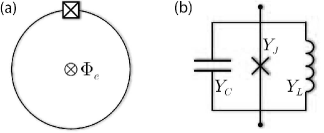
Figure 1: (a) Schematic representation of a qubit controlled by a magnetic flux, see Eq. (2). (b) Effective circuit diagram with three parallel elements – capacitor, Josephson junction, and inductor – characterized by their respective admittances.

The second term in Eq. (1) is the sum of the BCS Hamiltonians for quasiparticles in the leads

$$\hat{H}_{\mathrm{qp}}=\sum_{j=L,R}\hat{H}_{\mathrm{qp}}^{j}\,,\quad\hat{H}_{\mathrm{qp}}^{j}=\sum_{n,\sigma}\epsilon_{n}^{j}\hat{\alpha}^{j\dagger}_{n\sigma}\hat{\alpha}^{j}_{n\sigma},$$ (3)

where $\hat{\alpha}^{j}_{n\sigma}$($\hat{\alpha}^{j\dagger}_{n\sigma}$) are quasiparticle annihilation (creation) operators and $\sigma=\uparrow,\downarrow$ accounts for spin. The quasiparticle energies are $\epsilon^{j}_{n}=\sqrt{(\xi_{n}^{j})^{2}+(\Delta^{j})^{2}}$, with $\xi_{n}^{j}$ and $\Delta^{j}$ being the single-particle energy level $n$ in the normal state of lead $j$, and the gap parameter in that lead, respectively. The occupations of the quasiparticle states are described by the distribution functions

$$f^{j}(\xi^{j}_{n})=\langle\!\langle\hat{\alpha}_{n\uparrow}^{j\dagger}\hat{\alpha}^{j}_{n\uparrow}\rangle\!\rangle_{\mathrm{qp}}=\langle\!\langle\hat{\alpha}_{n\downarrow}^{j\dagger}\hat{\alpha}^{j}_{n\downarrow}\rangle\!\rangle_{\mathrm{qp}}\,,\quad j=L,R\,,$$ (4)

assumed to be independent of spin; double angular brackets $\langle\!\langle\ldots\rangle\!\rangle_{\mathrm{qp}}$ denote averaging over the quasiparticle states. Hereinafter we assume for simplicity equal gaps in the leads, $\Delta^{L}=\Delta^{R}\equiv\Delta$.

The last term in Eq. (1) describes quasiparticle tunneling across the junction and couples the phase and quasiparticle degrees of freedom

$$\hat{H}_{T}=\tilde{t}\!\!\sum_{n,m,\sigma}\!\!\left(e^{i\frac{\hat{\varphi}}{2}}u_{n}^{L}u_{m}^{R}-e^{-i\frac{\hat{\varphi}}{2}}v_{m}^{R}v_{n}^{L}\right)\hat{\alpha}_{n\sigma}^{L\dagger}\hat{\alpha}^{R}_{m\sigma}+\text{H.c.}\quad$$ (5)

The electron tunneling amplitude $t$ in this equation determines the junction conductance, $g_{T}=4\pi e^{2}\nu^{L}\nu^{R}\tilde{t}^{2}$ in the tunneling limit $\tilde{t}\ll 1$ which we are considering. From now on, we assume identical densities of states per spin direction in the leads, $\nu^{L}\!=\!\nu^{R}\!=\!\nu_{0}$. The Bogoliubov amplitudes $u^{j}_{n}$, $v^{j}_{n}$ can be taken real, since Eq. (5) already accounts explicitly for the phases of the order parameters in the leads via the gauge-invariant phase difference BP in the exponentials. Accounting for the Josephson effect and quasiparticles dynamics by Eqs. (2)-(5) is possible as long as the qubit energy $\omega$ and characteristic energy $\delta E$ of quasiparticles (as determined by their distribution function and measured from $\Delta$) are small compared to $\Delta$: lutchyn1 $\omega,\delta E\ll 2\Delta$. In this low-energy limit, we may further approximate $u^{j}_{m}\simeq v^{j}_{n}\simeq 1/\sqrt{2}$. Then the operators $e^{\pm i\hat{\varphi}/2}$ in Eq. (5), which describe transfer of charge $\pm e$ across the junction, combine to give

$$\hat{H}_{T}=\tilde{t}\!\!\sum_{n,m,\sigma}\!\!i\sin\frac{\hat{\varphi}}{2}\hat{\alpha}_{n\sigma}^{L\dagger}\hat{\alpha}^{R}_{m\sigma}+\text{H.c.}$$ (6)

Starting from this low-energy tunneling Hamiltonian, in the next section we calculate the dissipative part of the junction admittance.

II.1 Response to a classical time-dependent phase

We consider here the “classical” dissipative response of a Josephson junction to a small ac bias to show that Eq. (6) correctly accounts for the known BP junction losses in the low-energy regime. These “classical” losses are directly related to the decay rate in the quantum regime, as we explicitly show in the next section.

We assume a time-dependent bias $v(t)=v\cos(\omega t)$ of frequency $\omega>0$ superimposed to a fixed phase difference $\varphi_{0}$. In other words, we take the phase to be a time-dependent number which, by the Josephson equation $d\varphi/dt=2ev(t)$, has the form

$$\varphi(t)=\varphi_{0}+\frac{2ev}{\omega}\sin(\omega t)\,.$$ (7)

Here we focus on the linear in $v$ response in the low-energy regime. Expressions for the current through the junction valid beyond linear response can be found, for example, in Ref. BP, . Substituting Eq. (7) into Eq. (6), expanding for small $v$, and keeping the linear term, we find for the time-dependent perturbation $\delta\hat{H}(t)$ causing the dissipation

$$\begin{split}\delta\hat{H}(t)&=\hat{H}_{AC}\sin(\omega t)\,,\\ \hat{H}_{AC}&=i\tilde{t}\cos\frac{\varphi_{0}}{2}\frac{ev}{\omega}\sum_{n,m,\sigma}\hat{\alpha}_{n\sigma}^{L\dagger}\hat{\alpha}^{R}_{m\sigma}+\text{H.c.}\end{split}$$ (8)

The average dissipated power can be calculated using Fermi’s golden rule: it is given by the product of the transition rate times the energy change in a transition between quasiparticle states caused by the perturbation. The energy change in a transition is $\pm\omega$ by energy conservation, with the two signs corresponds to the events giving energy to or taking energy from the system. The average power $P$ is

$$P=2\pi\sum_{\left\{\lambda\right\}_{\mathrm{qp}}}\langle\!\langle\left|\langle\left\{\lambda\right\}_{\mathrm{qp}}|\hat{H}_{AC}|\left\{\eta\right\}_{\mathrm{qp}}\rangle\right|^{2}\omega$$ (9)

$$\times\left[\delta(E_{\lambda,\mathrm{qp}}-E_{\eta,\mathrm{qp}}-\omega)-\delta(E_{\lambda,\mathrm{qp}}-E_{\eta,\mathrm{qp}}+\omega)\right]\rangle\!\rangle_{\mathrm{qp}}\,,$$

where $E_{\eta,\mathrm{qp}}$ and $E_{\lambda,\mathrm{qp}}$ are the total energies of the quasiparticles in their respective initial $\{\eta\}_{\mathrm{qp}}$ and final $\{\lambda\}_{\mathrm{qp}}$ states. We use Eq. (8) to evaluate the matrix element, average over initial quasiparticle states, and sum over final states to find

$$P=\frac{1}{2}\mathrm{Re}\,Y_{J}(\omega,\varphi_{0})v^{2}$$ (10)

withcosphi

$$\mathrm{Re}\,Y_{J}(\omega,\varphi)=\frac{1+\cos\varphi}{2}\mathrm{Re}\,Y_{\mathrm{qp}}(\omega).$$ (11)

Here $\mathrm{Re}\,Y_{\mathrm{qp}}$ is the real part of the quasiparticle contribution to the junction admittance at zero phase difference,

$$\begin{split}\mathrm{Re}\,Y_{\mathrm{qp}}(\omega)=&g_{T}\frac{2\Delta}{\omega}\int_{0}^{\infty}\!dx\,\frac{1}{\sqrt{x}\sqrt{x+\omega/\Delta}}\\ &\left[f_{E}\left((1+x)\Delta\right)-f_{E}\left((1+x+\omega/\Delta)\Delta\right)\right].\end{split}$$ (12)

In deriving these formulas we have approximated the standard BCS density of states functions as

$$\frac{\epsilon}{\sqrt{\epsilon^{2}-\Delta^{2}}},\,\frac{\Delta}{\sqrt{\epsilon^{2}-\Delta^{2}}}\sim\sqrt{\frac{\Delta}{2(\epsilon-\Delta)}}\equiv\frac{1}{\sqrt{2x}}$$ (13)

and taken equal quasiparticle occupations in the two leads, $f^{L}=f^{R}\equiv f$; we use this simplifying assumption throughout the paper. We indicate with $f_{E}$ the energy mode of the distribution function

$$f_{E}(\epsilon)=\frac{1}{2}\left[f(\xi)+f(-\xi)\right],$$ (14)

where $\epsilon=\sqrt{\xi^{2}+\Delta^{2}}$. Equation (11) for the real part of the admittance, valid at $\omega>0$, agrees with the linear response, low-energy limit of the non-linear $I$-$V$ characteristic presented in Ref. BP, . Extension to $\omega<0$ is found by noticing that $\mathrm{Re}\,Y_{\mathrm{qp}}$ is an even function of frequency.

In thermal equilibrium and at low temperatures $T\ll\Delta$ the distribution function can be approximated as

$$f_{E}(\epsilon)\simeq e^{-\epsilon/T},$$ (15)

and Eq. (12) gives, at arbitrary ratio $\omega/T$,

$$\begin{split}\mathrm{Re}\,Y_{\mathrm{qp}}^{eq}(\omega)=g_{T}\frac{2\Delta}{\omega}e^{-\Delta/T}e^{\omega/2T}K_{0}\left(\frac{|\omega|}{2T}\right)\left[1-e^{-\omega/T}\right].\end{split}$$ (16)

Here $K_{0}$ is the modified Bessel function of the second kind with asymptotes

$$K_{0}(x)\simeq\left\{\begin{array}[]{lll}e^{-x}\sqrt{\pi/2x}\,,&&x\gg 1\\ \ln 2/x-\gamma_{E}\,,&&x\ll 1\end{array}\right.$$ (17)

with $\gamma_{E}$ the Euler gamma.

For a generic distribution function, we can relate $\mathrm{Re}\,Y_{\mathrm{qp}}$ to the density of quasiparticle $n_{\mathrm{qp}}$ in the high-frequency regime $\omega\gg\delta E$, where $\delta E$ indicates the characteristic energy of quasiparticle (measured from the gap) above which the occupation of the quasiparticle states can be neglected; in thermal equilibrium $\delta E\sim T$. Under the assumption $\omega\gg\delta E$ we obtain from Eq. (12)

$$\mathrm{Re}\,Y_{\mathrm{qp}}^{hf}(\omega)=\frac{1}{2}x_{\mathrm{qp}}\,g_{T}\left(\frac{2\Delta}{|\omega|}\right)^{3/2},$$ (18)

where

$$x_{\mathrm{qp}}=\frac{n_{\mathrm{qp}}}{2\nu_{0}\Delta}$$ (19)

is the quasiparticle density normalized to the Cooper pair density and

$$n_{\mathrm{qp}}=2\sqrt{2}\nu_{0}\Delta\int_{0}^{\infty}\frac{dx}{\sqrt{x}}f_{E}((1+x)\Delta)$$ (20)

is the density written using the approximation in Eq. (13). Note that in thermal equilibrium at low temperatures, Eq. (15), we have

$$n_{\mathrm{qp}}^{eq}=2\nu_{0}\sqrt{2\pi\Delta T}e^{-\Delta/T}.$$ (21)

Then using Eq. (17), it is easy to check that for $T\ll\omega$ Eq. (16) takes the form given in Eq. (18).

The real and imaginary parts of the admittance satisfy the Kramers-Krönig relations. However, when taking the Kramers-Krönig transform of the real part, a purely inductive contribution to the imaginary part can be missed. Indeed, at low energies the complex junction admittance (obtained from the expressions in Ref. BP, ) can be written as

$$Y_{J}(\omega,\varphi)=\frac{1-2x^{\mathrm{A}}_{\mathrm{qp}}}{i\omega L_{J}}\cos\varphi+Y_{\mathrm{qp}}(\omega)\frac{1+\cos\varphi}{2}\,,$$ (22)

where

$$x^{\mathrm{A}}_{\mathrm{qp}}=f_{E}(\Delta)$$ (23)

can be interpreted as the population of the Andreev bound states beenakker and the inverse of the Josephson inductance is

$$\frac{1}{L_{J}}=g_{T}\pi\Delta_{\mathrm{qp}}$$ (24)

(the subscript $\mathrm{qp}$ in $\Delta_{\mathrm{qp}}$ is used to indicate that in this expression it may be necessary to account for the effect of quasiparticles on the gap, see Secs. II.3 and III.2).

Unlike the Andreev states, free quasiparticles contribute to both dissipative and non-dissipative parts of the total admittance $Y_{J}$ via the complex term $Y_{\mathrm{qp}}$. The real part of the quasiparticle admittance is defined in Eq. (12), while its imaginary part is given by the Kramers-Krönig transform of that expression,

$$\begin{split}\mathrm{Im}\,Y_{\mathrm{qp}}(\omega)=-g_{T}\frac{2\Delta}{\omega}\frac{P}{\pi}\int_{0}^{\infty}\!\frac{dx}{\sqrt{x}}\int_{0}^{\infty}\!\frac{dy}{\sqrt{y}}\Big{[}f_{E}\left((1+x)\Delta\right)\\ -f_{E}\left((1+y)\Delta\right)\Big{]}\left[\frac{1}{x-y+\omega/\Delta}-\frac{1}{x-y}\right],\end{split}$$ (25)

where $P$ denotes the principal part and $\omega>0$. Using that $\mathrm{Im}\,Y_{\mathrm{qp}}$ is an odd function of frequency, we can simplify the above expression to a form with a single rather than double integral

$$\mathrm{Im}\,Y_{\mathrm{qp}}(\omega)=g_{T}\frac{2\Delta}{\omega}\left[\int_{0}^{|\omega|/\Delta}\!\!dx\,\frac{f_{E}\left((1+x)\Delta\right)}{\sqrt{x}\sqrt{|\omega|/\Delta-x}}-\pi x^{\mathrm{A}}_{\mathrm{qp}}\right].$$ (26)

As discussed above for the real part, an analytic expression for $\mathrm{Im}\,Y_{\mathrm{qp}}$ can be obtained in thermal equilibrium,

$$\mathrm{Im}\,Y_{\mathrm{qp}}^{eq}(\omega)=-g_{T}\frac{2\Delta}{\omega}e^{-\Delta/T}\pi\left[1-e^{-|\omega|/2T}I_{0}\left(\frac{|\omega|}{2T}\right)\right].$$ (27)

Here $I_{0}$ is the modified Bessel function of the first kind with asymptotes

$$I_{0}(x)\simeq\left\{\begin{array}[]{lll}e^{x}\sqrt{1/2\pi x}\,,&&x\gg 1\\ 1+x^{2}/4\,,&&x\ll 1\end{array}\right..$$ (28)

For arbitrary distribution function satisfying the high-frequency condition $\omega\gg\delta E$ we find

$$\mathrm{Im}\,Y_{\mathrm{qp}}^{hf}(\omega)=\frac{1}{2}g_{T}\,\frac{2\Delta}{\omega}\left[x_{\mathrm{qp}}\sqrt{\frac{2\Delta}{|\omega|}}-2\pi x^{\mathrm{A}}_{\mathrm{qp}}\right].$$ (29)

Using Eq. (21) and the large-$x$ limit in Eq. (28), it is easy to show that for $T\ll\omega$ Eq. (27) reduces to the general expression in Eq. (29). In the high-frequency regime, real and imaginary parts of the quasiparticle admittance can be combined into the complex admittance

$$Y_{\mathrm{qp}}^{hf}(\omega)=-\frac{2}{i\omega L_{J}}\left[\frac{x_{\mathrm{qp}}}{\pi}\sqrt{\frac{\Delta}{i\omega}}-x^{\mathrm{A}}_{\mathrm{qp}}\right].$$ (30)

By substituting Eq. (30) into Eq. (22) we find that in the total admittance $Y_{J}$ the coefficient multiplying $x^{\mathrm{A}}_{\mathrm{qp}}$ is proportional to $(1-\cos\varphi)$ and vanishes for $\varphi=0$. This is in agreement with the absence of Andreev bound states when there is no phase difference across the junction.

II.2 Transition rates

The effects of the interaction between quasiparticles and qubit degree of freedom, Eq. (5), can be treated perturbatively in the tunneling amplitude $\tilde{t}$. The interaction makes possible, for example, a transition between two qubit states (initial, $|i\rangle$, and final, $|f\rangle$, differing in energy by amount $\omega_{if}>0$) by exciting a quasiparticle during a tunneling event. The rate for the transition between qubit states can be calculated using Fermi’s golden rule

$$\begin{split}\Gamma_{i\to f}=2\pi\sum_{\{\lambda\}_{\mathrm{qp}}}&\langle\!\langle\left|\langle f,\{\lambda\}_{\mathrm{qp}}|\hat{H}_{T}|i,\{\eta\}_{\mathrm{qp}}\rangle\right|^{2}\\ &\ \times\delta\left(E_{\lambda,\mathrm{qp}}-E_{\eta,\mathrm{qp}}-\omega_{if}\right)\rangle\!\rangle_{\mathrm{qp}}\,.\end{split}$$ (31)

We remind that in our notation $E_{\eta,\mathrm{qp}}$ ($E_{\lambda,\mathrm{qp}}$) is the total energy of the quasiparticles in their initial (final) state $\{\eta\}_{\mathrm{qp}}$ ($\{\lambda\}_{\mathrm{qp}}$), and double angular brackets $\langle\!\langle\ldots\rangle\!\rangle_{\mathrm{qp}}$ denote averaging over the initial quasiparticle states whose occupation is determined by the distribution function.

In the low-energy regime we are considering, the transition rate factorizes into terms accounting separately for qubit dynamic and quasiparticle kinetics

$$\Gamma_{i\to f}=\left|\langle f|\sin\frac{\hat{\varphi}}{2}|i\rangle\right|^{2}S_{\mathrm{qp}}\left(\omega_{if}\right).$$ (32)

Equation (32) is one of the main results of this work: it shows that the qubit properties affect the transition rate via the wavefunctions $|i\rangle$, and $|f\rangle$ entering the matrix element, while the quasiparticle kinetics is accounted for by the quasiparticle current spectral density $S_{\mathrm{qp}}$

$$\begin{split}S_{\mathrm{qp}}\left(\omega\right)=&\frac{16E_{J}}{\pi}\int_{0}^{\infty}\!\!\!dx\,\frac{1}{\sqrt{x}\sqrt{x+\omega/\Delta}}\Big{[}f_{E}\left((1+x)\Delta\right)\\ &\times\left(1-f_{E}\left((1+x)\Delta+\omega\right)\right)\Big{]},\end{split}$$ (33)

where $\omega>0$ and we used the relation

$$E_{J}=g_{T}\Delta/8g_{K}$$ (34)

with $g_{K}=e^{2}/2\pi$ the conductance quantum. The expression for $S_{\mathrm{qp}}$ at $\omega<0$ is obtained by the replacements $x\to x-\omega/\Delta$, $\omega\to-\omega$ in the integrand in Eq. (33).

The spectral density $S_{\mathrm{qp}}$ depends on the detail of the distribution functions. In thermal equilibrium at low temperatures $T\ll\Delta$, using Eq. (15) we find

$$S_{\mathrm{qp}}^{eq}(\omega)=\frac{16E_{J}}{\pi}e^{-\Delta/T}e^{\omega/2T}K_{0}\left(\frac{|\omega|}{2T}\right).$$ (35)

Note that the equality

$$\frac{S_{\mathrm{qp}}^{eq}(-\omega)}{S_{\mathrm{qp}}^{eq}(\omega)}=e^{-\omega/T}$$ (36)

implies that in thermal equilibrium the transition rates are related by detailed balance,

$$\frac{\Gamma_{f\to i}}{\Gamma_{i\to f}}=e^{-\omega_{if}/T}.$$ (37)

The similarity between Eq. (35) for $S_{\mathrm{qp}}$ and Eq. (16) for $\mathrm{Re}\,Y_{\mathrm{qp}}$ is not accidental. In thermal equilibrium the following fluctuation-dissipation relation holds

$$S_{\mathrm{qp}}^{eq}(\omega)+S_{\mathrm{qp}}^{eq}(-\omega)=\frac{\omega}{\pi}\frac{1}{g_{K}}\mathrm{Re}\,Y_{\mathrm{qp}}^{eq}(\omega)\coth\left(\frac{\omega}{2T}\right).$$ (38)

Moreover, in the low-energy regime for an arbitrary distribution function the two quantities are also related by

$$S_{\mathrm{qp}}(\omega)-S_{\mathrm{qp}}(-\omega)=\frac{\omega}{\pi}\frac{1}{g_{K}}\mathrm{Re}\,Y_{\mathrm{qp}}(\omega)\,.$$ (39)

In the high-frequency regime $\omega\gg\delta E$, we can simplify the above relation to

$$S_{\mathrm{qp}}^{hf}(\omega)=\frac{\omega}{\pi}\frac{1}{g_{K}}\mathrm{Re}\,Y_{\mathrm{qp}}^{hf}(\omega).$$ (40)

For the transition rates this corresponds to neglecting the downward transitions with $\omega_{if}<0$, in which a quasiparticle looses energy to the qubit, compared to the upward ones. This is a good approximation since the assumption $\omega\gg\delta E$ means that there are no quasiparticles with energy high enough to excite the qubit. Equation (40) can be checked by comparing Eq. (18) to

$$S_{\mathrm{qp}}^{hf}(\omega)=x_{\mathrm{qp}}\frac{8E_{J}}{\pi}\sqrt{\frac{2\Delta}{\omega}}$$ (41)

with $E_{J}$ given in Eq. (34) and the the normalized quasiparticle density $x_{\mathrm{qp}}$ in Eq. (19).

II.3 Energy level corrections

In addition to causing transitions between qubit levels, the quasiparticles affect the energy $E_{i}$ of each level $i$ of the system. We can distinguish two quasiparticle mechanisms that modify the qubit spectrum and hence separate two terms in the correction $\delta E_{i}$ to the energy,

$$\delta E_{i}=\delta E_{i,E_{J}}+\delta E_{i,\mathrm{qp}}\,.$$ (42)

First, in the presence of quasiparticles the Josephson energy takes the form

$$E_{J,\mathrm{qp}}=\frac{g_{T}}{8g_{K}}\Delta_{\mathrm{qp}}(1-2x^{\mathrm{A}}_{\mathrm{qp}})$$ (43)

with $x^{\mathrm{A}}_{\mathrm{qp}}$ defined in Eq. (23). As mentioned after Eq. (24), we use $\Delta_{\mathrm{qp}}$ to distinguish the self-consistent gap in the presence of quasiparticles from the gap $\Delta$ when there are no quasiparticles. At leading order in the quasiparticle density we have

$$\Delta_{\mathrm{qp}}\simeq\Delta\left(1-x_{\mathrm{qp}}\right).$$ (44)

Treating these modifications to the Josephson energy as perturbations, the correction to the energy of level $i$ is

$$\delta E_{i,E_{J}}=E_{J}\left(x_{\mathrm{qp}}+2x^{\mathrm{A}}_{\mathrm{qp}}\right)\langle i|\cos\hat{\varphi}|i\rangle\,.$$ (45)

Second, the virtual transitions between the qubit levels mediated by quasiparticle tunneling cause a correction that can be expressed in terms of the matrix elements of $\sin\hat{\varphi}/2$ as

$$\begin{split}\delta E_{i,\mathrm{qp}}=\sum_{k\neq i}\left|\langle k|\sin\frac{\hat{\varphi}}{2}|i\rangle\right|^{2}F_{\mathrm{qp}}\left(\omega_{ik}\right)\,,\end{split}$$ (46)

where

$$\omega_{ik}=E_{k}-E_{i}\,.$$ (47)

The derivation of the above formulas and the definition of function $F_{\mathrm{qp}}$ in terms of the quasiparticle distribution function [Eq. (159)] are given in Appendix A. Here we give the relation between $F_{\mathrm{qp}}$ and the imaginary part of the quasiparticle impedance,

$$F_{\mathrm{qp}}(\omega)+F_{\mathrm{qp}}(-\omega)=-\frac{\omega}{2\pi}\frac{1}{g_{K}}\mathrm{Im}\,Y_{\mathrm{qp}}(\omega),$$ (48)

which we will use in the next section to obtain the quasiparticle-induced change in the qubit frequency.

III Single junction: weakly anharmonic qubit

As an application of the general approach described in the previous section, we consider here a weakly anharmonic qubit, such as the transmon and phase qubits. We start with the the semiclassical limit, i.e., we assume that the potential energy terms in Eq. (2) dominate the kinetic energy term proportional to $E_{C}$. This limit already reveals a non-trivial dependence of relaxation on flux. Note that assuming $E_{L}\neq 0$ we can eliminate $n_{g}$ in Eq. (2) by a gauge transformation.flux_th In the transmon we have $E_{L}=0$ and the spectrum depends on $n_{g}$, displaying both well separated and nearly degenerate states, see Fig. 2. The results of this section can be applied to the single-junction transmon when considering well separated states. The transition rate between these states and the corresponding frequency shift are dependent on $n_{g}$. However, since $E_{C}\ll E_{J}$ this dependence introduces only small corrections to $\Gamma_{n\to n-1}$ and $\delta\omega$; the corrections are exponential in $-\sqrt{8E_{J}/E_{C}}$. By contrast, the leading term in the rate of transitions $\Gamma_{e\leftrightarrow o}$ between the even and odd states is exponentially small. The rate $\Gamma_{e\leftrightarrow o}$ of parity switching is discussed in detail in Appendix C.

Figure 2: Schematic representation of the transmon low energy spectrum as function of the dimensionless gate voltage $n_{g}$. Solid (dashed) lines denotes even (odd) states (see also Sec. IV.1). The amplitudes of the oscillations of the energy levels are exponentially small,transmon see Appendix B; here they are enhanced for clarity. Quasiparticle tunneling changes the parity of the qubit sate. The results of Sec. III are valid for transitions between states separated by energy of the order of the plasma frequency $\omega_{p}$, Eq. (56), and give, for example, the rate $\Gamma_{1\to 0}$. For the transition rates between nearly degenerate states of opposite parity, such as $\Gamma^{(1)}_{o\to e}$, see Appendix C.

The potential energy in Eq. (2) is extremized at phase $\varphi_{0}$ satisfying

$$E_{J}\sin\varphi_{0}+E_{L}\left(\varphi_{0}-2\pi\Phi_{e}/\Phi_{0}\right)=0.$$ (49)

For $E_{J}<E_{L}$ there is only one solution at the global minimum. For $E_{J}>E_{L}$ however, there can be multiple minima; their number depends both on the ratio $E_{J}/E_{L}$ and the external flux $\Phi_{e}$. Here we assume that the flux is such that distinct minima are not degenerate; in particular, this means that the flux is tuned away from odd integer multiples of half the flux quantum.noteEL For the transmon with $E_{L}=0$, we can take $\varphi_{0}=0$ as solution to Eq. (49). Next, we expand the potential energy around a minimum and find at quadratic order

$$\hat{H}^{(2)}_{\varphi}=4E_{C}\hat{n}^{2}+\frac{1}{2}\left(E_{L}+E_{J}\cos\varphi_{0}\right)\left(\hat{\varphi}-\varphi_{0}\right)^{2}.$$ (50)

Fluctuations of the phase around $\varphi_{0}$ are small under the assumption

$$n\frac{E_{C}}{\omega_{10}}\ll 1,$$ (51)

where $n$ denotes the energy level and

$$\omega_{10}=\sqrt{8E_{C}\left(E_{L}+E_{J}\cos\varphi_{0}\right)}$$ (52)

is the qubit frequency in the harmonic approximation. Note that anharmonicity and quality factor $Q$ determine the operability of the system as a qubit. Dev_rev The anharmonic correction to the transition frequencies can be calculated by considering the effect on the spectrum of the next order in the expansion around $\varphi_{0}$ (cubic for the phase qubit, quartic for the transmon), which defines an anharmonic potential well of finite depth $U$. Then the operability condition can be expressed as $Q/n_{w}\gg 1$, where $n_{w}$ is the number of states in the potential well, $n_{w}\sim U/\omega_{10}$.note1 In a weakly anharmonic system, $n_{w}$ can be large; however, if the quality factor is larger the system can be used as a qubit despite the weak anharmonicity, as it is indeed the case for the transmon. transmon

The condition for small phase fluctuations in Eq. (51) enables us to calculate the matrix element of operator $\sin\hat{\varphi}/2$ by expanding around $\varphi_{0}$ up to the second order and using standard expressions for the matrix elements of the position operator between eigenstates $|n\rangle$, $|m\rangle$ of the harmonic oscillator [cf. Eq. (50)]. To first order in $E_{C}/\omega_{10}$ we find (see also Appendix D)

$$\begin{split}&\left|\langle m|\sin\frac{\hat{\varphi}}{2}|n\rangle\right|^{2}=\delta_{m,n}\left[1-2\frac{E_{C}}{\omega_{10}}\left(n+\frac{1}{2}\right)\right]\frac{1-\cos\varphi_{0}}{2}\\ &\hskip 39.83368pt+\frac{E_{C}}{\omega_{10}}\left[n\delta_{m,n-1}+\left(n+1\right)\delta_{m,n+1}\right]\frac{1+\cos\varphi_{0}}{2}\,.\end{split}$$ (53)

Note that in the first term on the right hand side the corrections due to the non-linearity of sine (the second term inside the square brackets) are indeed small if condition (51) is satisfied. In addition, we have neglected here the anharmonic corrections to the states used to calculate the matrix element; this is a good approximation for low-lying levels $n\ll n_{w}$.note2 For the transmon ($\varphi_{0}=0$) the leading term in Eq. (53) is of linear order in $E_{C}/\omega_{10}\ll 1$; as we show in Appendix E by including the first anharmonic correction to the states, the next non-vanishing term in the square of the transmon matrix element is cubic in $E_{C}/\omega_{10}$, rather than quadratic as for the harmonic oscillator. Therefore in the case of the transmon keeping only the leading term is a better approximation than naively expected.

Equation (53) shows that at leading order we can restrict our attention to transitions involving only neighboring levels. Concentrating here on low-lying levels, using Eqs. (32), (39), and (53) we find the following relation between transition rate and impedance

$$\Gamma_{n\to n-1}-\Gamma_{n-1\to n}=\frac{n}{C}\mathrm{Re}\,Y_{\mathrm{qp}}(\omega_{10})\frac{1+\cos\varphi_{0}}{2},$$ (54)

where we also used $E_{C}=e^{2}/2C$. In the high-frequency regime, the upward transition rate can be neglected, $\Gamma_{n-1\to n}\simeq 0$, and the above expression simplifies tok_corr [see also Eq. (40) and the text that follows it]

$$\begin{split}\Gamma_{n\to n-1}&=\frac{n}{C}\mathrm{Re}\,Y_{\mathrm{qp}}^{hf}(\omega_{10})\frac{1+\cos\varphi_{0}}{2}\\ &=n\frac{\omega_{p}^{2}}{\omega_{10}}\frac{x_{\mathrm{qp}}}{2\pi}\sqrt{\frac{2\Delta}{\omega_{10}}}\left(1+\cos\varphi_{0}\right)\,.\end{split}$$ (55)

In the last expression we used Eq. (18) and introduced the plasma frequency

$$\omega_{p}=\sqrt{8E_{C}E_{J}}\,.$$ (56)

The above equation can also be obtained by substituting directly Eq. (40) into Eq. (32). For $n=1$ and $\varphi_{0}=0$ Eq. (55) reduces to the transition rate presented in Ref. Martinis, .

The transition rate in Eq. (55) is proportional to the (possibly non-equilibrium) quasiparticle density $x_{\mathrm{qp}}$ and depends on the external flux $\Phi_{e}$ via $\varphi_{0}$ and $\omega_{10}$, see Eqs. (49) and (52). The flux dependence is in general sensitive to the states involved in the transition. This sensitivity can already be seen for transitions between harmonic oscillator states: due to the non-linear interaction between phase and quasiparticles, see Eq. (6), transitions between distant levels are possible. These transitions are suppressed by the smallness of phase fluctuations when $E_{C}/\omega_{10}\ll 1$. For example, the rate for the $2\to 0$ transition is

$$\!\!\Gamma_{2\to 0}=\frac{2\omega_{10}}{\pi}\frac{1}{g_{K}}\mathrm{Re}\,Y_{\mathrm{qp}}^{hf}(2\omega_{10})\!\left(\frac{E_{C}}{\omega_{10}}\right)^{2}\!\frac{1-\cos\varphi_{0}}{4}.$$ (57)

Note that in contrast to Eq. (55), Eq. (57) cannot be written in terms of the real part of the total admittance of the junction: while in Eq. (55) the phase enters via the factor $(1+\cos\varphi_{0})$ as in Eq. (11), in Eq. (57) $\mathrm{Re}\,Y_{\mathrm{qp}}$ is multiplied by $(1-\cos\varphi_{0})$. To obtain $\Gamma_{2\to 0}$ we substituted into Eq. (32) the high-frequency relation (40), while the explicit form of the squared matrix element $|\langle 0|\sin(\hat{\varphi}/2)|2\rangle|^{2}$ is found by setting $n=2$, and keeping the leading term in $E_{C}/\omega_{10}$, in the formula

$$\left|\langle 0|\sin\frac{\hat{\varphi}}{2}|n\rangle\right|^{2}=e^{-\frac{E_{C}}{\omega_{10}}}\left(\frac{E_{C}}{\omega_{10}}\right)^{n}\frac{1-(-1)^{n}\cos\varphi_{0}}{2n!}$$ (58)

derived in Appendix D. Equation (58) is valid for any ratio $E_{C}/\omega_{10}$ for transitions between eigenstates of the harmonic oscillator. When $\varphi_{0}=0$, Eq. (58) gives vanishing matrix elements for even $n$ – this is an example of the more general selection rule according to which only transitions between states of different parity are allowed at $\varphi_{0}=0$.

The rate for transitions between excited states and the ground state in the case of large phase fluctuations can be obtained using Eq. (58) when $E_{L}\ll E_{C}$ and $E_{J}\lesssim\omega_{LC}=\sqrt{8E_{C}E_{L}}$. The latter condition enables us to neglect the Josephson energy term in Eq. (2). Then using Eqs. (32) and (41) with $\omega_{if}=n\omega_{LC}$ we find that the transition rate has a maximum for $n=n_{0}$ with $n_{0}\approx E_{C}/\omega_{LC}$,

$$\begin{split}\Gamma_{n\to 0}\simeq&\,\frac{\omega_{p}^{2}}{E_{C}}\frac{x_{\mathrm{qp}}}{2\pi}\sqrt{\frac{2\Delta}{E_{C}}}\left[1-(-1)^{n}\cos 2\pi\Phi_{e}/\Phi_{0}\right]\\ &\times\frac{1}{\sqrt{2\pi n_{0}}}\exp\left[-\frac{(n-n_{0})^{2}}{2n_{0}}\right].\end{split}$$ (59)

Here we have approximated $e^{-y}y^{n}/n!\sqrt{n}\simeq\exp[-(n-y)^{2}/2y]/\sqrt{2\pi}\,y$; the approximation is valid for $y\gg 1$ and $|n-y|\lesssim\sqrt{2y}$. Equation (59) shows that when the charging energy is the dominant energy scale, dissipation is the strongest for transitions between states whose energy difference ($n\omega_{LC}$) corresponds to the energy change ($E_{C}$) caused by the transfer of a single electron through the barrier, as in the “quasiparticle poisoning” picture for the Cooper pair box. lutchyn1 We stress that in the present case charge is not quantized, due to the finite value of the inductive energy $E_{L}$.flux_th We will comment on the relation between Eq. (59) and the transition rate in the Cooper pair box in Sec. IV.1.

III.1 Quality factor

Returning now to the semiclassical regime of small $E_{C}$, Eq. (55) with $n=1$ enables us to evaluate, in the high-frequency regime, the inverse $Q$-factor for the transition between the qubit states

$$\frac{1}{Q_{10}}=\frac{\Gamma_{1\to 0}}{\omega_{10}}=\frac{1}{\pi g_{K}}\mathrm{Re}\,Y_{\mathrm{qp}}^{hf}(\omega_{10})\frac{E_{C}}{\omega_{10}}\frac{1+\cos\varphi_{0}}{2}\,.$$ (60)

We stress that this formula is valid not only in thermal equilibrium, but also in the presence of non-equilibrium quasiparticles with characteristic energy $\delta E\ll\omega_{10}$. We can generalize Eq. (60) to account for the possible coexistence of non-equilibrium and thermal quasiparticles. We take the distribution function in the form

$$f_{E}(\epsilon)=f_{ne}(\epsilon)+f_{eq}(\epsilon)\,,$$ (61)

where $f_{ne}$ is the non-equilibrium contribution, insensitive to temperature and satisfying the high-frequency condition $\omega_{10}\gg\delta E$, and $f_{eq}$ is the equilibrium distribution of Eq. (15). Noting that within our assumption the two terms in $f_{E}$ contribute separately to the transition rates and that for the thermal part we cannot in general neglect the “upward” transitions, using Eqs. (32), (35), (41), and (53) we find

$$\begin{split}\frac{1}{Q_{10}}=\frac{\Gamma_{1\to 0}+\Gamma_{0\to 1}}{\omega_{10}}=\frac{1+\cos\varphi_{0}}{2\pi}\frac{\omega_{p}^{2}}{\omega_{10}^{2}}\bigg{[}x_{ne}\sqrt{\frac{2\Delta}{\omega_{10}}}&\\ +4e^{-\Delta/T}\cosh\left(\frac{\omega_{10}}{2T}\right)K_{0}\left(\frac{\omega_{10}}{2T}\right)\bigg{]},&\end{split}$$ (62)

where $x_{ne}$ is the normalized non-equilibrium quasiparticle density [cf. Eq. (19)].

Recently good agreement between theory, Eq. (62), and experiment has been shown for single-junction transmons ($\varphi_{0}=0$, $\omega_{10}=\omega_{p}$) in the temperature range 10-210 mK. paik However, while these measurements indicate that thermal quasiparticles are the main cause of relaxation above $\sim 150$ mK, one cannot conclude that non-equilibrium quasiparticles are present from the lower temperature data: by Matthiessen rule, any other relaxation mechanism which is independent of (or weakly dependent on) temperature would have the same limiting effect on $Q_{10}$ as the first term in square brackets in Eq. (62). As we will discuss in more detail in Sec. V.1, similar measurements on a flux-sensitive device should enable one to decide on the presence of non-equilibrium quasiparticles, since Eq. (62) [and its analogous for the split transmon, Eq. (127)] describes the effect of flux on both equilibrium and non-equilibrium quasiparticle contributions to $Q_{10}$, and other sources of relaxation respond differently to the flux.

III.2 Frequency shift

A further test of the theory presented in Sec. II is provided by the measurement of the qubit resonant frequency. In the semiclassical regime of small $E_{C}$, the qubit can be described by the effective circuit of Fig. 1(b), with the junction admittance $Y_{J}$ of Eq. (22), $Y_{C}=i\omega C$, and $Y_{L}=1/i\omega L$ [the inductance is related to the inductive energy by $E_{L}=(\Phi_{0}/2\pi)^{2}/L$]. As discussed in Ref. prl, , for parallel elements the total admittance $Y$ is the sum of their admittances,

$$Y=Y_{J}+Y_{C}+Y_{L}\,,$$ (63)

and the resonant frequency $\omega_{r}$ is the zero of the total admittance, $Y(\omega_{r})=0$. In the absence of quasiparticles we find $\omega_{r}=\omega_{10}$ with $\omega_{10}$ of Eq. (52).

In the presence of quasiparticles, by considering their effect on the junction admittance at linear order in the quasiparticle density $x_{\mathrm{qp}}$ and Andreev level occupation $x^{\mathrm{A}}_{\mathrm{qp}}$ we obtain

$$\omega_{r}=\omega_{10}+\delta\omega$$ (64)

with

$$\begin{split}\delta\omega=\frac{i}{2C}Y_{\mathrm{qp}}(\omega_{10})\frac{1+\cos\varphi_{0}}{2}-\frac{\pi g_{T}\Delta}{C\omega_{10}}x^{\mathrm{A}}_{\mathrm{qp}}\cos\varphi_{0}\\ -\frac{\pi g_{T}\Delta}{2C\omega_{10}}x_{\mathrm{qp}}\cos\varphi_{0}\,.\end{split}$$ (65)

The last term in Eq. (65) originates from the gap suppression by quasiparticles [cf. Eq. (44)]. This term was neglected in Ref. prl, as it is subleading in the high-frequency regime considered there [see Eq. (73)]. The correction $\delta\omega$ has both real and imaginary parts. The imaginary part coincidesprl with half the dissipation rate in Eq. (55) for the $n=1\to 0$ transition. Here we show that the real part of $\delta\omega_{r}$ obtained in the effective circuit approach agrees with the quantum mechanical calculation.

Within the harmonic approximation of Eq. (50), the energy difference $\omega_{i}$ between the neighboring levels $E_{i+1}$ and $E_{i}$,

$$\omega_{i}\equiv E_{i+1}-E_{i}=\omega_{10}\,,$$ (66)

is of course independent of the level index $i$. The quasiparticle corrections to energy levels of Sec. II.3 cause a correction $\delta\omega_{i}$ to $\omega_{i}$,

$$\delta\omega_{i}=\delta E_{i+1}-\delta E_{i}\,.$$ (67)

As we show below, at leading order in $E_{C}/\omega_{10}$ this correction is also independent of level index, i.e, it represents a renormalization of the system resonant frequency.

As in Eq. (42), we separate the contributions due to change in the Josephson energy and due to quasiparticle tunneling,

$$\delta\omega_{i}=\delta\omega_{i,E_{J}}+\delta\omega_{i,\mathrm{qp}}.$$ (68)

For the first term on the right hand side, we use Eq. (45) together with the matrix element of $\cos\hat{\varphi}$ at first order in $E_{C}/\omega_{10}$ [see Eq. (211)],

$$\langle i|\cos\hat{\varphi}|i\rangle\simeq\cos\varphi_{0}\left[1-\frac{4E_{C}}{\omega_{10}}\left(i+\frac{1}{2}\right)\right],$$ (69)

to find

$$\delta\omega_{i,E_{J}}=-\frac{1}{2}\frac{\omega_{p}^{2}}{\omega_{10}}\cos\varphi_{0}\left(x_{\mathrm{qp}}+2x^{\mathrm{A}}_{\mathrm{qp}}\right)\,.$$ (70)

As discussed in Sec. II.3, the term proportional to $x_{\mathrm{qp}}$ is due to the gap suppression in the presence of quasiparticles, Eq. (44), while $x^{\mathrm{A}}_{\mathrm{qp}}$ accounts for the occupation of the Andreev bound states.

For the quasiparticle tunneling term, we substitute Eq. (53) into Eq. (46) to get

$$\delta\omega_{i,\mathrm{qp}}=\frac{E_{C}}{\omega_{10}}\left[F_{\mathrm{qp}}(\omega_{10})+F_{\mathrm{qp}}(-\omega_{10})\right]\frac{1+\cos\varphi_{0}}{2}\,.$$ (71)

Finally, using the relation (48) and adding the two terms we arrive at

$$\begin{split}\delta\omega_{i}=&-\frac{1}{2C}\mathrm{Im}\,Y_{\mathrm{qp}}(\omega_{10})\frac{1+\cos\varphi_{0}}{2}\\ &-\frac{1}{2}\frac{\omega_{p}^{2}}{\omega_{10}}\cos\varphi_{0}\left(x_{\mathrm{qp}}+2x^{\mathrm{A}}_{\mathrm{qp}}\right)\,.\end{split}$$ (72)

This expression agrees with the real part of Eq. (65). We note that by extending the above consideration to include the next order in $E_{C}/\omega_{10}$, anharmonic corrections to the spectrum can be calculated. They are dominated by the anharmonicity of the cosine potential in Eq. (2), with quasiparticles contributing negligible additional corrections. For the case of the transmon, the leading anharmonicity can be found in Ref. transmon, .

In the high-frequency regime, using Eq. (29) the relative frequency shift is

$$\begin{split}\frac{\delta\omega_{i}}{\omega_{10}}=&\frac{1}{2}\frac{\omega_{p}^{2}}{\omega_{10}^{2}}\Bigg{[}x^{\mathrm{A}}_{\mathrm{qp}}\left(1-\cos\varphi_{0}\right)\\ &-x_{\mathrm{qp}}\left(\frac{1+\cos\varphi_{0}}{2\pi}\sqrt{\frac{2\Delta}{\omega_{10}}}+\cos\varphi_{0}\right)\Bigg{]}.\end{split}$$ (73)

Note that in the limit $\omega_{10}\ll\Delta$ we can neglect the cosine compared to the term multiplied by square root inside round brackets. However, this cosine term is the appropriate subleading contribution, since the terms neglected in deriving the energy corrections presented in Sec. II.3 are suppressed by $\omega_{10}/\Delta$ with respect to the leading contribution.

In recent experiments with single-junction transmons paik relative shifts of order $10^{-5}$ have been measured at temperatures $\sim 200$ mK, in agreement with Eq. (72). Together with the above mentioned measurements of the transition rates in the same devices, this is an additional, independent check of the validity of the present theory in the regime $T\gtrsim 150$ mK. While in the transmon ($\varphi_{0}=0$) there are no Andreev bound states [indeed, in this case their contribution to the frequency shift is absent, see Eq. (73)], in a phase qubit both Andreev levels occupation $x^{\mathrm{A}}_{\mathrm{qp}}$ and free quasiparticle density $x_{\mathrm{qp}}$ affect the frequency. Assuming that the two quantity are proportional, $x^{\mathrm{A}}_{\mathrm{qp}}\propto x_{\mathrm{qp}}$ ,the ratio between frequency shift, Eq. (73), and transition rate, Eq. (55), in the high frequency regime is independent of the quasiparticle density. The constancy of this ratio has been recently verified by injecting a variable (but unknown) number quasiparticles in a phase qubit. martinis2

IV Single junction: strong anharmonicity

Here we consider the regime, complementary to that of the previous section, of qubits with large anharmonicities. We study first the single junction Cooper pair box (CPB); as for the transmon, it is insensitive to flux, but in contrast to the transmon the CPB properties are strongly affected by the value of the dimensionless gate voltage $n_{g}$. Then we analyze a flux qubit, for which the external flux is tuned near half the flux quantum, $\Phi_{e}\approx\Phi_{0}/2$.

IV.1 Cooper pair box

The CPB is described by Eq. (2) with $E_{L}=0$ and $E_{C}\gg E_{J}$. In this limit, it is convenient to rewrite the Hamiltonian in the charge basis as lutchyn1

$$\begin{split}\hat{H}=&\,E_{C}\sum_{q}\Big{(}q-2n_{g}\Big{)}^{2}|q\rangle\langle q|\\ &-\frac{1}{2}E_{J}\sum_{q}\Big{(}|q\rangle\langle q+2|+|q+2\rangle\langle q|\Big{)}.\end{split}$$ (74)

The eigenstates have definite parity (even/odd) and are given by linear combinations of even/odd charge states. The CPB operating point is, without loss of generality, at $n_{g}=1/2$. Near this operating point, the CPB is well described by the reduced Hamiltonian

$$H_{CPB}=\left(\begin{matrix}E_{C}(2n_{g})^{2}&0&-E_{J}/2\\ 0&E_{C}(2n_{g}-1)^{2}&0\\ -E_{J}/2&0&E_{C}(2n_{g}-2)^{2}\end{matrix}\right).$$ (75)

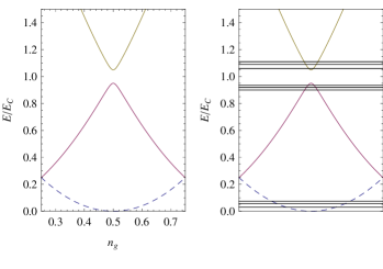
Figure 3: Left panel: spectrum of the reduced CPB Hamiltonian, Eq. (75), around the operating point $n_{g}=1/2$ for $E_{J}=0.1E_{C}$. Dashed line: energy of the odd state, Eq. (77). Solid lines: energies of ground (bottom) and excited (top) even states, Eq. (78). Right panel: in the presence of a small inductive energy $E_{L}$, the CPB bands act as potentials in the quasimomentum space, see Ref. flux_th, . Dense horizontal lines represent a few energy levels near the edges of the bands.

The reduced CPB Hamiltonian has a single odd eigenstate, the $|q=1\rangle$ charge state,

$$|o,0;n_{g}\rangle=|1\rangle,$$ (76)

with $n_{g}$-dependent eigenenergy

$$E_{0}(n_{g})=E_{C}(2n_{g}-1)^{2}\,,$$ (77)

and two even eigenstates, $|e,\pm;n_{g}\rangle$, with energies

$$E_{\pm}(n_{g})=E_{C}+E_{0}(n_{g})\pm\frac{1}{2}\omega_{10}(n_{g})\,.$$ (78)

The qubit frequency depends on the gate voltage as

$$\omega_{10}(n_{g})=\sqrt{(4E_{C})^{2}(2n_{g}-1)^{2}+E_{J}^{2}}\,.$$ (79)

Note that at the operating point we have $\omega_{10}(1/2)=E_{J}$ and that the frequency rises quickly at a narrow distance from the optimal point, more than doubling for $|n_{g}-1/2|\sim E_{J}/E_{C}\ll 1$. In terms of the charge states, the two even eigenstates are

$$\begin{split}|e,-;n_{g}\rangle&=\cos\theta|0\rangle+\sin\theta|2\rangle\,,\\ |e,+;n_{g}\rangle&=\sin\theta|0\rangle-\cos\theta|2\rangle\,,\end{split}$$ (80)

where

$$\cos\theta=\frac{1}{\sqrt{2}}\sqrt{1-\frac{4E_{C}(2n_{g}-1)}{\omega_{10}(n_{g})}}.$$ (81)

The non-vanishing matrix elements of $\sin\hat{\varphi}/2$ can be readily obtained using the charge basis form of this operator

$$\sin\frac{\hat{\varphi}}{2}=\frac{1}{2i}\sum_{q}\Big{(}|q+1\rangle\langle q|-|q\rangle\langle q+1|\Big{)}.$$ (82)

For the states in Eqs. (76) and (80) we find

$$\left|\langle o,0;n_{g}|\sin\frac{\hat{\varphi}}{2}|e,\pm;n_{g}\rangle\right|^{2}=\frac{1}{4}\left[1\pm\frac{E_{J}}{\omega_{10}(n_{g})}\right].$$ (83)

We stress that the transitions are not between the qubit (i.e., even) states, but between the even and odd states; the corresponding transition frequencies are $\omega_{\pm}(n_{g})=E_{C}\pm\omega_{10}(n_{g})/2$, see Eqs. (77) and (78). Therefore the tunneling of a quasiparticle into the CPB changes the parity of the state, an effect known as “quasiparticle poisoning”. matveev Substituting the matrix element (83) into Eq. (32) and using the high-frequency expression (41) we find

$$\Gamma_{e,+\to o,0}=\left[1+\frac{E_{J}}{\omega_{10}(n_{g})}\right]\frac{2E_{J}}{\pi}\,x_{\mathrm{qp}}\sqrt{\frac{2\Delta}{\omega_{+}(n_{g})}}$$ (84)

for the transition between even excited and odd states. In thermal equilibrium with $T\ll\omega_{+}(n_{g})$, using Eq. (21) we obtain

$$\Gamma_{e,+\to o,0}=\left[1+\frac{E_{J}}{\omega_{10}(n_{g})}\right]\frac{4E_{J}}{\sqrt{\pi}}\sqrt{\frac{T}{\omega_{+}(n_{g})}}e^{-\Delta/T}.$$ (85)

Within our approximations, this expression reproduces (after implementing the corrections described in Ref. erratum, and up to a numerical prefactor) the decay rate calculated in Ref. lutchyn1, for the “open” qubit at the operating point $n_{g}=1/2$. For the transition between even ground and odd states the matrix element in Eq. (83) vanishes at the operating point. This vanishing is a consequence of the low-energy approximation that lead to Eq. (6): as the results of Refs. lutchyn1, ; lutchyn2, show, the contributions that we neglect cause a finite transition rate, which is suppressed by a small factor of order $E_{C}/2\Delta$ in comparison with the transition rate from even excited to odd state.

We note that while in all the above expressions the distance $|2n_{g}-1|$ from the operating point can be large compared to the small parameter $E_{J}/E_{C}\ll 1$, the description based on Eq. (75) is valid if other charge states can be neglected, which limits the range of validity to $|2n_{g}-1|<1/2$ (with $|2n_{g}-1|-1/2\gg E_{J}/E_{C}$). For example, at $2n_{g}-1\simeq 1/2$ the charge states $|0\rangle$ and $|3\rangle$ are nearly degenerate and we can expect an enhanced transition rate $\Gamma_{e,+\to o,3}$ in comparison to the rate $\Gamma_{e,+\to o,0}$ that we have considered above.

Finally, let us comment on the relationship between the transition rate in the CPB and in the inductively shunted Josephson junction with large charging energy [see the paragraph containing Eq. (59)]. As shown schematically in the right panel of Fig. 3 and discussed in detail in Ref. flux_th, , the spectra of the two systems are distinct even in the limit of small inductive energy $E_{L}$: in the CPB ($E_{L}=0$) the energy levels form bands as $n_{g}$ varies, while for any non-zero $E_{L}$ the gate voltage $n_{g}$ can be “gauged away” and the spectrum consists of discrete levels that become denser as $E_{L}$ decreases. Despite these differences, the ac responses of the two systems due to charge coupling agree in this limit.flux_th Similarly, we now show agreement for the quasiparticle transition rates. We note that when taking the limit $E_{L}\to 0$, the condition $E_{J}\lesssim\omega_{LC}$ for the validity of Eq. (59) for the rate $\Gamma_{n\to 0}$ requires that we also take $E_{J}\to 0$. cpbcomp Moreover, since the final state considered in deriving the rate $\Gamma_{n\to 0}$ is the lowest possible state, the corresponding final state in the CPB is either the even ground state at $n_{g}=0$ or the odd ground state at $n_{g}=1/2$. Indeed, the width of the ground state (in quasimomentum space – see Fig. 3 and Ref. flux_th, ) is $\propto(E_{L}/E_{C})^{1/4}$, so that as $E_{L}\to 0$ the state is localized at the bottom of the band. Note that following the same procedure detailed above it is straightforward to show that the transition rate $\Gamma_{o,+\to e,0}$ at $n_{g}=0$ coincides with $\Gamma_{e,+\to o,0}$ at $n_{g}=1/2$; hence for our purposes the two possibilities are equivalent. At finite $E_{L}$, the total transition rate to the ground state is obtained by summing Eq. (59) over all initial levels $n$. Due to the Gaussian factor in the second line of Eq. (59), the number of levels that contribute to the total rate is approximately $\sqrt{n_{0}}\propto(E_{C}/E_{L})^{1/4}$, which grows as the inductive energy diminishes. However, the energy of the contributing levels tends to the charging energy, as can be seen by rewriting identically the argument in the exponential of the Gaussian factor as $-(E_{n}-E_{C})^{2}/2E_{C}\omega_{LC}$, where $E_{n}=n\omega_{LC}$; this agrees with frequency for the $e,+\to o,0$ transition at $n_{g}=1/2$ in the CPB being approximately $E_{C}$ in the small $E_{J}$ limit. Using Eq. (59), performing the sum over levels, and taking the limit $E_{L}\to 0$, we find

$$\lim_{E_{L}\to 0}\sum_{n}\Gamma_{n\to 0}=\frac{4E_{J}}{\pi}\,x_{\mathrm{qp}}\sqrt{\frac{2\Delta}{E_{C}}}\,,$$ (86)

which coincides with the leading term of Eq. (84) in the limit $E_{J}\to 0$ at the operating point $n_{g}=1/2$.

IV.2 Flux qubit

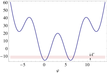
Figure 4: Potential energy (in units of $E_{L}$) for a flux qubit biased at $\Phi_{e}=\Phi_{0}/2$ with $E_{J}/E_{L}=10$. The horizontal lines represent the two lowest energy levels, with energy difference $\bar{\epsilon}$ given in Eq. (100).

As a second example of a strongly anharmonic system, we consider here a flux qubit, i.e., in Eq. (2) we assume $E_{J}>E_{L}$ and take the external flux to be close to half the flux quantum, $\Phi_{e}\approx\Phi_{0}/2$. Then the potential has a double-well shape and the flux qubit ground states $|-\rangle$ and excited state $|+\rangle$ are the lowest tunnel-split eigenstates in this potential,Dev_rev see Fig. 4. The non-linear nature of the $\sin\hat{\varphi}/2$ qubit-quasiparticle coupling in Eq. (6) has a striking effect on the transition rate $\Gamma_{+\to-}$, which vanishes at $\Phi_{e}=\Phi_{0}/2$ due to destructive interference: for flux biased at half the flux quantum the qubit states $|-\rangle$, $|+\rangle$ are respectively symmetric and antisymmetric around $\varphi=\pi$, while the potential in Eq. (2) and the function $\sin\varphi/2$ in Eq. (32) are symmetric. Note that the latter symmetry and its consequences are absent in the environmental approach in which a linear phase-quasiparticle coupling is assumed.

Analytic evaluation of the matrix element determining the transition rate [Eq. (32)] at finite $\Phi_{e}-\Phi_{0}/2$ is possible when $E_{C}\ll E_{J}$ and the tunnel splitting $\bar{\epsilon}$ is small compared to inductive and plasma energies, $\bar{\epsilon}\ll 2\pi^{2}E_{L}\ll\omega_{p}$; an estimate for the splitting is given below in Eq. (100). With the above assumptions we can use a tight-binding approach. Neglecting tunneling the wavefunctions $|m\rangle$ are, as a first approximation, ground state wavefunctions of the harmonic oscillator with frequency $\omega_{p}$ and oscillator length $\ell=\sqrt{8E_{C}/\omega_{p}}$ localized around the (flux-dependent) minima $\varphi_{m}$ of the potential energy,

$$\langle\varphi|m\rangle=\left(\frac{1}{\pi\ell^{2}}\right)^{1/4}e^{-(\varphi-\varphi_{m})^{2}/2\ell^{2}}.$$ (87)

The minima are found by solving Eq. (49) approximately, using the condition $E_{L}\ll E_{J}$ (which follows from the above assumptions) to get

$$\varphi_{m}\simeq 2\pi\left[m-\frac{E_{L}}{E_{J}}(m-f)\right]\,,\qquad f=\frac{\Phi_{e}}{\Phi_{0}}\,.$$ (88)

The energies of the localized states are (up to a constant term)

$$E_{m}=2\pi^{2}\bar{E}_{L}(m-f)^{2}\,,$$ (89)

where

$$\bar{E}_{L}=E_{L}\left(1-\frac{1}{\beta}\right)\,,\qquad\beta=\frac{E_{J}}{E_{L}}$$ (90)

takes into account corrections small in $1/\beta\ll 1$. The above results are valid for $|mE_{L}/E_{J}|\ll 1$. Still neglecting tunneling, the matrix element of $\sin\hat{\varphi}/2$ between states localized in different wells vanishes, but the diagonal matrix element is finite due to the shift of the minima away from $2\pi m$, see Eq. (88). Using the states in Eq. (87) we obtain

$$\langle j|\sin\frac{\hat{\varphi}}{2}|m\rangle\simeq-(-1)^{m}\pi\frac{E_{L}}{E_{J}}(m-f)\delta_{m,j}\,.$$ (91)

To include the effect of tunneling we allow for the possibility of transitions between neighboring wells with amplitude $\bar{\epsilon}/2$. As we are interested in the two lowest eigenstates for $f$ near 1/2, we consider only the $m=0,1$ wells and the effective Hamiltonian has the form

$$\hat{H}=\left(\begin{matrix}2\pi^{2}\bar{E}_{L}f^{2}&-\bar{\epsilon}/2\\ -\bar{\epsilon}/2&2\pi^{2}\bar{E}_{L}(1-f)^{2}\end{matrix}\right).$$ (92)

The eigenenergies are [cf. Eqs. (78)-(81)]

$$E_{\pm}(f)=\frac{\pi^{2}}{2}\bar{E}_{L}\left[1+(2f-1)^{2}\right]\pm\frac{1}{2}\omega_{10}(f)$$ (93)

with the flux-dependent qubit frequency

$$\omega_{10}(f)=\sqrt{\bar{\epsilon}^{2}+\left[(2\pi)^{2}\bar{E}_{L}(f-1/2)\right]^{2}}\,,$$ (94)

while the eigenstates are

$$\begin{split}|-\rangle&=\cos\theta|0\rangle+\sin\theta|1\rangle\,,\\ |+\rangle&=\sin\theta|0\rangle-\cos\theta|1\rangle\,,\end{split}$$ (95)

with

$$\cos\theta=\frac{1}{\sqrt{2}}\sqrt{1-\frac{(2\pi)^{2}\bar{E}_{L}(f-1/2)}{\omega_{10}(f)}}\,.$$ (96)

The tunnel splitting $\bar{\epsilon}$ entering in the above formulas can be estimated by noting that due to the assumption $\beta\gg 1$ the wells are nearly symmetric. Neglecting the asymmetry [i.e., considering the potential in Eq. (2) at $f=1/2$], the width and height of the tunnel barrier are approximately $2\pi(1-1/\beta)$ and $2\bar{E}_{J}$, respectively, with

$$\bar{E}_{J}=E_{J}\left[1-\frac{\pi^{2}}{4}\frac{1}{\beta}\left(1-\frac{1}{\beta}\right)\right].$$ (97)

To account for the height and width at $E_{L}\neq 0$, we treat the two wells as cosine potentials with renormalized coefficients. That is, we consider each well to be described by the Hamiltonian given in Eq. (170) with the substitutions $E_{J}\to\bar{E}_{J}$ and $E_{C}\to\bar{E}_{C}$, where

$$\bar{E}_{C}=E_{C}\frac{1}{\left(1-1/\beta\right)^{2}}.$$ (98)

Then we can use the known asymptotic formula transmon ; flux_th ; jcp for the splitting $\epsilon_{0}$ in the periodic cosine potential (i.e., for $E_{L}=0$; see Appendix B for a derivation of this formula)

$$\epsilon_{0}=4\sqrt{\frac{2}{\pi}}\,\omega_{p}\left(\frac{8E_{J}}{E_{C}}\right)^{1/4}e^{-\sqrt{8E_{J}/E_{C}}}$$ (99)

to find

$$\bar{\epsilon}=2\sqrt{\frac{2}{\pi}}\sqrt{8\bar{E}_{J}\bar{E}_{C}}\left(\frac{8\bar{E}_{J}}{\bar{E}_{C}}\right)^{1/4}e^{-\sqrt{8\bar{E}_{J}/\bar{E}_{C}}}.$$ (100)

Here the numerical prefactor is smaller by factor of 2 in comparison with Eq. (99) to account for tunneling being between two wells rather than in a periodic potential. jcp

Turning now to the matrix element $\langle j|\sin\hat{\varphi}/2|m\rangle$, the diagonal elements $j=m=0,\,1$ are still approximately given by Eq. (91). Tunneling introduces finite but exponentially small off-diagonal elements which, similarly to the splitting, can be calculated using the semiclassical approximation. Using the wavefunctions derived in Appendix B we arrive at [cf. Eq. (195)]

$$\langle 1|\sin\frac{\hat{\varphi}}{2}|0\rangle\simeq D\left(\frac{\bar{E}_{J}}{\bar{E}_{C}}\right)^{1/3}\frac{\bar{\epsilon}}{2\sqrt{2}\bar{E}_{J}}$$ (101)

with $D\approx 1.45$, see Eq. (196). We can now calculate the matrix element of $\sin\hat{\varphi}/2$ between qubit states $|\pm\rangle$ in Eq. (95) using Eqs. (91) and (101) to obtain

$$\begin{split}\langle-|\sin\frac{\hat{\varphi}}{2}|+\rangle=\pi(f-1/2)\frac{\bar{\epsilon}}{\omega_{10}(f)}\qquad\\ \times\left[\frac{E_{L}}{E_{J}}+\sqrt{2}\pi D\frac{\bar{E}_{L}}{\bar{E}_{J}}\left(\frac{\bar{E}_{J}}{\bar{E}_{C}}\right)^{1/3}\right].\end{split}$$ (102)

Here the first term in square brackets is the combination of the two intrawell contributions [Eq. (91)] while the second one originates from the under-barrier tunneling [Eq. (101)]. Comparing Eq. (102) to numerical calculations, we find that near half the flux quantum, $|f-1/2|\lesssim\bar{\epsilon}/2\pi^{2}E_{L}$, the two approaches give the same dependence on flux and agree on the order of magnitude of the matrix element, with Eq. (102) providing a smaller estimate than the numerics by a factor of about $2/3$. For $|f-1/2|\gtrsim\bar{\epsilon}/(2\pi)^{2}E_{L}$ the flux dependence in Eq. (102) via the factor $(f-1/2)/\omega_{10}(f)$ can be neglected and the right hand side reduces to a flux-independent constant. However, this behavior is an artifact of our approximations: for these larger deviations of flux from half the flux quantum the matrix element acquires additional flux dependence, beyond that given in Eq. (102), once the asymmetry of the potential is taken into account. Moreover, for very small flux, $|f|\lesssim(\bar{\epsilon}/4\sqrt{2}\pi^{2}E_{L})^{2}$, mixing of the sate localized in well $m=1$ with that localized in well $m=-1$ cannot be neglected and the matrix element has a narrow peak around zero flux. Substituting Eq. (102) into Eq. (32), keeping the leading contribution, and using the relation (40), we find for the transition rate in the high-frequency regimemf

$$\begin{split}\Gamma_{+\to-}=\frac{\omega_{10}}{\pi}\frac{1}{g_{K}}\mathrm{Re}\,Y^{hf}_{\mathrm{qp}}(\omega_{10})\left(\frac{\bar{\epsilon}}{4\pi\bar{E}_{J}}\right)^{2}\left(1-\frac{\bar{\epsilon}^{2}}{\omega_{10}^{2}}\right)\\ \left(\sqrt{2}\pi D\right)^{2}\left(\frac{\bar{E}_{J}}{\bar{E}_{C}}\right)^{2/3}\end{split}$$ (103)

with $\mathrm{Re}\,Y^{hf}_{\mathrm{qp}}$ of Eq. (18).

The rate in Eq. (103) depends on reduced flux $f$ via the qubit frequency, see Eq. (94). In particular, for external flux equaling half the flux quantum we have $\omega_{10}(1/2)=\bar{\epsilon}$ and the transition rate vanishes, as discussed above. In the previous section we mentioned in the text after Eq. (85) that for the Cooper pair box the vanishing of the rate at the operating point is valid up to small corrections, being a consequence of the low-energy approximation for the tunneling Hamiltonian in Eq. (6). The same is true for the flux qubit; in the present case, the parameter suppressing these corrections is exponentially small, being given by $\bar{\epsilon}/2\Delta$. Note that if keeping in Eq. (5) the contributions beyond the low energy approximation, the operators accounting for the qubit-quasiparticle interaction cannot be reduced to $\sin\hat{\varphi}/2$; therefore, for these additional contributions the symmetry argument given at the beginning of this section for the vanishing of the transition rate at $f=1/2$ does not hold.

V Multiple-junction qubits: general theory and applications

In this section we generalize the theory of Sec. II to the case of systems containing multiple junctions. This generalization will enables us to consider the flux dependence of the transition rates in the two-junction split transmon and in the many-junction fluxonium. These two qubits are particular examples of the general case in which $M+1$ junctions separate $M+1$ superconducting islands forming a loop. We use the convention that junction $j=0,\ldots,M$ is between islands $j$ and $j+1$ and identify island $j=M+1$ with island $j=0$ – see Fig. 5. When the loop inductive energy is much larger than the Josephson energies of the junctions (i.e., the loop inductance is small), the phases are subject to the flux quantization constraint

$$\sum_{j=0}^{M}\varphi_{j}=2\pi\Phi_{e}/\Phi_{0}\,.$$ (104)

This constraint must be taken into account to derive the Hamiltonian $\hat{H}_{\{\phi\}}$ of the $M$ independent phase degrees of freedom $\phi$, $\phi_{k}$ ($k=1,\ldots,M-1$) starting from the Lagrangianngnote ${\cal L}_{\{\varphi\}}$ for the $M+1$ constrained phases $\varphi_{j}$

$${\cal L}_{\{\varphi\}}=\sum_{j=0}^{M}\left[\frac{1}{2}C_{j}\left(\frac{\Phi_{0}}{2\pi}\dot{\varphi}_{j}\right)^{2}+E_{Jj}\cos\varphi_{j}\right],$$ (105)

where the dot denotes derivative with respect to time, $C_{j}$ is the capacitance of junction $j$, and $E_{Jj}$ its Josephson energy. In Appendix F we derive the Hamiltonian assuming $M$ of the $M+1$ junctions to be identical, which is relevant for both the split transmon ($M=1$) and the fluxonium ($M\gg 1$). Explicit expressions for the Hamiltonian in these two cases are presented below.

The total Hamiltonian $\hat{H}$ of the system consist of three terms, as in Eq. (1):

$$\hat{H}=\hat{H}_{\{\phi\}}+\hat{H}_{\mathrm{qp}}+\hat{H}_{T}\,.$$ (106)

In addition to $\hat{H}_{\{\phi\}}$ discussed above, the second contribution is the quasiparticle Hamiltonian

$$\hat{H}_{\mathrm{qp}}=\sum_{j=0}^{M}\hat{H}_{\mathrm{qp}}^{j}\,,\quad\hat{H}_{\mathrm{qp}}^{j}=\sum_{n,\sigma}\epsilon_{n}^{j}\hat{\alpha}^{j\dagger}_{n\sigma}\hat{\alpha}^{j}_{n\sigma}\,.$$ (107)

Here the index $j$ denotes the superconducting island; other symbols have the same meaning as in Eq. (3) and we assume equal gaps in all islands, $\Delta^{j}\equiv\Delta$. The final contribution to $\hat{H}$ is the tunnel Hamiltonian, given by the following sum [cf. Eq. (6)]

$$\hat{H}_{T}=\sum_{j=0}^{M}\tilde{t}_{j}\!\!\sum_{n,m,\sigma}\!\!i\sin\frac{\hat{\varphi}_{j}}{2}\hat{\alpha}_{n\sigma}^{j\dagger}\hat{\alpha}^{j+1}_{m\sigma}+\text{H.c.}$$ (108)

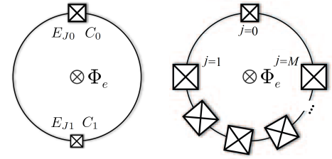
Figure 5: Left: schematic representation of the split transmon with two (possibly different) junctions. Right: in the fluxonium a weaker junction ($j=0$) is connected to a large junction array ($j=1,\ldots,M$).

The transition rate between qubit states can again be calculated using Fermi’s golden rule as in Eq. (31). We assume that the quasiparticle distribution functions are the same in all islands and that tunneling across each junction is not correlated with tunneling in nearby junctions – this is a good assumption if the mean level spacing in the finite size superconductors is small compared to the gap. Then the total rate for the transition between eigenstates of Hamiltonian $\hat{H}_{\{\phi\}}$ is

$$\Gamma_{i\to f}=\sum_{j=0}^{M}\left|\langle f_{\{\phi\}}|\sin\frac{\hat{\varphi}_{j}}{2}|i_{\{\phi\}}\rangle\right|^{2}E_{Jj}\tilde{S}_{\mathrm{qp}}\left(\omega_{if}\right),$$ (109)

where for convenience we have extracted the Josephson energy prefactor from the spectral density, $\tilde{S}_{\mathrm{qp}}=S_{\mathrm{qp}}/E_{J}$, with $S_{\mathrm{qp}}$ defined in Eq. (33). Similarly, the correction $\delta E_{i}$ to the energy of state $i_{\{\phi\}}$ is given by sums over junctions which generalize Eqs. (45) and (46),

$$\delta E_{i} = \delta E_{i,E_{J}}+\delta E_{i,\mathrm{qp}}\,,$$ (110)

$$\delta E_{i,E_{J}} = \sum_{j=0}^{M}E_{Jj}\langle i_{\{\phi\}}|\cos\hat{\varphi}_{j}|i_{\{\phi\}}\rangle(x_{\mathrm{qp}}+2x^{\mathrm{A}}_{\mathrm{qp}})\,,$$ (111)

$$\delta E_{i,\mathrm{qp}} = \sum_{j=0}^{M}E_{Jj}\!\sum_{k\neq i}\left|\langle k_{\{\phi\}}|\sin\frac{\hat{\varphi}_{j}}{2}|i_{\{\phi\}}\rangle\right|^{2}\!\tilde{F}_{\mathrm{qp}}(\omega_{ik}),\quad\quad\$$ (112)

where $\tilde{F}_{\mathrm{qp}}=F_{\mathrm{qp}}/E_{J}$. In the next subsections we use Eq. (109) to calculate the transition rates for the split transmon and the fluxonium, and Eq. (110) to find the frequency shift in the split transmon. The flux-dependent transition rate between the two lowest even and odd states of a split Cooper pair box has been recently considered in Ref. schon, for gate voltage tuned at the operating point.

V.1 Split transmon

A split transmon consists of two junctions, $j=0,1$, in a superconducting loop, see Fig. 5. Therefore, there is only $M=1$ degree of freedom, which we denote with $\phi$, governed by the Hamiltonian

$$\hat{H}_{\phi}=4E_{C}\hat{N}^{2}-E_{J0}\cos(\hat{\phi}-2\pi f)-E_{J1}\cos\hat{\phi}\,,$$ (113)

see Appendix F. Here $\hat{N}=-id/d\phi$, $f=\Phi_{e}/\Phi_{0}$, and the charging energy $E_{C}$ is related to the junctions’ capacitances by

$$E_{C}=\frac{e^{2}}{2(C_{0}+C_{1})}\,.$$ (114)

Note that the Hamiltonian is periodic in $f$ with period 1, so we can assume $|f|\leq 1/2$ without loss of generality (i.e., we can measure the normalized flux from the nearest integer). After shifting $\phi\to\phi+\pi f$, the sum of the two Josephson terms can be rewritten as

$$E_{J0}\cos(\hat{\phi}-2\pi f)+E_{J1}\cos\hat{\phi}\to E_{J}(f)\cos(\hat{\phi}-\vartheta)\,,$$ (115)

where the effective Josephson energy $E_{J}$ is modulated by the external flux

$$E_{J}(f)=\left(E_{J0}+E_{J1}\right)\cos(\pi f)\sqrt{1+d^{2}\tan^{2}(\pi f)}$$ (116)

with

$$d=\frac{E_{J0}-E_{J1}}{E_{J0}+E_{J1}}$$ (117)

and

$$\tan\vartheta=d\tan(\pi f).$$ (118)

After a further shift $\phi\to\phi+\vartheta$ we arrive at

$$\hat{H}_{\phi}=4E_{C}\hat{N}^{2}-E_{J}(f)\cos\hat{\phi}\,,$$ (119)

which has the same form of the Hamiltonian for the single junction transmon [i.e., Eq. (2) with $E_{L}=0$] but with a flux-dependent Josephson energy, Eq. (116). Therefore the spectrum follows directly from that of the single junction transmon (see Fig. 2) and consists of nearly degenerate and well separated states. The energy difference between well separated states is approximately given by the flux-dependent frequency [cf. Eq. (56)]

$$\omega_{p}(f)=\sqrt{8E_{C}E_{J}(f)}.$$ (120)

Note that for the system to be in the transmon regime

$$E_{J}(f)\gg E_{C}$$ (121)

at some flux, a necessary condition is

$$E_{J0}+E_{J1}\gg E_{C}\,.$$ (122)

Then we can distinguish two cases. First, in the nearly symmetric case of junctions with comparable Josephson energies, $|E_{J0}-E_{J1}|\lesssim E_{C}$, the condition (121) is satisfied not too close to half the flux quantum,

$$|f|-1/2\gg E_{C}/\pi(E_{J0}+E_{J1}).$$ (123)

On the other hand, if the Josephson energies are sufficiently different, $|E_{J0}-E_{J1}|\gg E_{C}$, then Eq. (121) is satisfied at any flux.

The transition rate $\Gamma_{1\to 0}$ between the qubit states $|0\rangle$, $|1\rangle$ can be calculated using Eq. (109) if we know the relation between $\varphi_{j}$ and $\phi$; the same relation is also needed to calculate the transition rate $\Gamma_{o\to e}$ between nearly degenerate states – see Appendix C.2 for details. According to Appendix F, for the variable $\phi$ in Eq. (113) we have $\varphi_{1}=\phi$ and $\varphi_{0}=2\pi f-\phi$. Accounting for the two changes of variables performed to arrive at Eq. (119) we obtain

$$\begin{split}\hat{\varphi}_{0}&=\pi f-\vartheta-\hat{\phi}\,,\\ \hat{\varphi}_{1}&=\pi f+\vartheta+\hat{\phi}\,.\end{split}$$ (124)

In the transmon regime (121), we proceed as in the derivation of Eq. (53) to find

$$\left|\langle 0|\sin\frac{\hat{\varphi}_{j}}{2}|1\rangle\right|^{2}=\frac{E_{C}}{\omega_{p}(f)}\frac{1+\cos(\pi f\pm\vartheta)}{2}\,,$$ (125)

where the upper (lower) sign is to be used for $j=1$ ($j=0$). Substituting this result into Eq. (109) and using Eq. (41) with $\omega=\omega_{p}(f)$, we find in the high frequency regime [cf. Eq. (55)]

$$\Gamma_{1\to 0}=\frac{x_{\mathrm{qp}}}{2\pi}\sqrt{\frac{2\Delta}{\omega_{p}(f)}}\frac{\omega_{p}^{2}(f)+\omega_{p}^{2}(0)}{\omega_{p}(f)}\,.$$ (126)

For the transition quality factor we consider, as in Sec. III.1, the coexistence of equilibrium and non-equilibrium quasiparticles [see Eq. (61)] to find

$$\begin{split}&\frac{1}{Q_{10}}=\frac{1}{2\pi}\left(1+\frac{\omega_{p}^{2}(0)}{\omega_{p}^{2}(f)}\right)\bigg{[}x_{ne}\sqrt{\frac{2\Delta}{\omega_{p}(f)}}\\ &+4e^{-\Delta/T}\cosh\left(\frac{\omega_{p}(f)}{2T}\right)K_{0}\left(\frac{\omega_{p}(f)}{2T}\right)\bigg{]}.\end{split}$$ (127)

In Fig. 6 we show with solid lines the quality factor as function of temperature for 4 different values of flux $f$ in a symmetric transmon (d=0). As we discussed in Sec. III.1, an extrinsic relaxation mechanism could be limiting the low temperature quality factor. Characterizing this mechanism by a constant quality factor $Q_{\mathrm{ext}}$ and assuming that only equilibrium quasiparticles are present, the transition quality factor has the form

$$\begin{split}\frac{1}{Q_{10,\mathrm{tot}}}=&\,\frac{1}{Q_{\mathrm{ext}}}+\frac{2}{\pi}\left(1+\frac{\omega_{p}^{2}(0)}{\omega_{p}^{2}(f)}\right)\\ &\times e^{-\Delta/T}\cosh\left(\frac{\omega_{p}(f)}{2T}\right)K_{0}\left(\frac{\omega_{p}(f)}{2T}\right).\end{split}$$ (128)

The dashed lines in Fig. 6 show $Q_{10,\mathrm{tot}}$ as a function of temperature for the same values of flux; the quality factor $Q_{\mathrm{ext}}$ is chosen so that the zero-flux curve coincides with the zero flux-curve described by Eq. (127). The change of quality factor with flux is markedly different in the two limiting cases (namely, presence of non-equilibrium quasiparticles and no extrinsic relaxation mechanism vs. extrinsic relaxation with no non-equilibrium quasiparticles) described by Eqs. (127) and (128). Therefore the measurement of the temperature and flux dependencies of the quality factor should give indications on the presence of non-equilibrium quasiparticles. For example, the low-temperature measurements reported in Ref. Houck, are compatible with a flux-independent quality factor; to explain the data with Eq. (127) rather than Eq. (128) one would need to assume a quasiparticle density that decreases with increasing flux. Since magnetic fields are known to break pairs and thus increase the quasiparticle density, for the transmons considered in Ref. Houck, it is unlikely that non-equilibrium quasiparticles are the source of the low-temperature qubit decay.

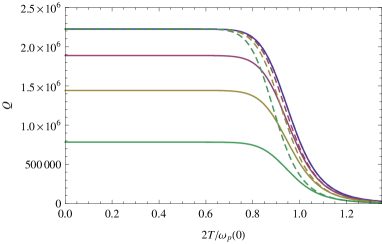
Figure 6: Quality factor as function of $2T/\omega_{p}(0)$ in a symmetric split transmon. Solid lines are obtained from Eq. (127) using a small nonequilibrium quasiparticle density $x_{ne}=3.8\times 10^{-7}$ and a gap value such that $\Delta/\omega_{p}(0)=6.9$ (these parameters are taken from experiments on single junction transmonpaik ). Flux increases from top to bottom; we show curves for $f=0$, $0.2$, $0.3$, and $0.4$, respectively. We plot Eq. (128) with dashed lines for the same values of flux. The extrinsic quality factor is chosen so that solid and dashed lines match at $f=0$.

The frequency shift for the split transmon is obtained, as in Sec. III.2, by calculating the difference between correction to energies of nearby levels, Eq. (67). The matrix elements appearing in Eqs. (111)-(112) are given by Eqs. (53) and (69) with $\omega_{10}=\omega_{p}(f)$, $\varphi_{0}=\theta+\pi f$ for $j=1$, and $\varphi_{0}=\theta-\pi f$ for $j=0$ [cf. Eq. (124)-(125)]. Using those expressions we find

$$\delta E_{i+1,E_{J}}-\delta E_{i,E_{J}}=-\frac{1}{2}\omega_{p}(f)\left(x_{\mathrm{qp}}+2x^{\mathrm{A}}_{\mathrm{qp}}\right)$$ (129)

and

$$\begin{split}\delta E_{i+1,\mathrm{qp}}-\delta E_{i,\mathrm{qp}}=\frac{1}{16}\frac{\omega_{p}^{2}(0)+\omega_{p}^{2}(f)}{\omega_{p}(f)}\\ \left[\tilde{F}_{\mathrm{qp}}(\omega_{p}(f))+\tilde{F}_{\mathrm{qp}}(-\omega_{p}(f))\right].\end{split}$$ (130)

Then using the relation (48) and Eq. (29), we arrive at the high frequency result

$$\begin{split}\frac{\delta\omega(f)}{\omega_{p}(f)}&\,=\frac{1}{2}\Bigg{\{}x^{\mathrm{A}}_{\mathrm{qp}}\left(\frac{\omega_{p}^{2}(0)}{\omega_{p}^{2}(f)}-1\right)\\ &-x_{\mathrm{qp}}\left[\frac{1}{2\pi}\left(\frac{\omega_{p}^{2}(0)}{\omega_{p}^{2}(f)}+1\right)\sqrt{\frac{2\Delta}{\omega_{p}(f)}}+1\right]\Bigg{\}}.\end{split}$$ (131)

At zero flux this expression agrees with Eq. (73) applied to a single junction transmon ($\omega_{10}=\omega_{p}$, $\varphi_{0}=0$). However, similarly to the flux qubit, at finite flux the split transmon frequency shift is sensitive to the occupation of the Andreev bound states, see the first term in curly brackets.

V.2 Fluxonium

In the fluxonium, an array of many identical junctions ($M\gg 1$) of Josephson energy $E_{J1}\gg E_{C1}$ is connected to a weaker junction with $E_{J0}<E_{J1}$. Then the Hamiltonian $\hat{H}_{\{\phi\}}$ for the $M$ independent degrees of freedom can be approximately separated into independent terms for the qubit phase $\phi$ and the $M-1$ phases $\phi_{k}$,

$$\hat{H}_{\{\phi\}} = \hat{H}_{\phi}+\sum_{k=1}^{M-1}\hat{H}_{k}\,,$$ (132)

$$\hat{H}_{\phi} = 4E_{C}\hat{N}^{2}-E_{J0}\cos\hat{\phi}+\frac{1}{2}E_{L}(\hat{\phi}-2\pi f)^{2},$$

$$\hat{H}_{k} = 4E_{C1}\hat{N}_{k}^{2}+\frac{1}{2}E_{J1}\hat{\phi}_{k}^{2}\,,$$

where

$$E_{L}=\frac{E_{J1}}{M},\qquad\frac{1}{E_{C}}=\frac{1}{E_{C0}}+\frac{1}{ME_{C1}},$$ (133)

see Appendix F. There, we also give [Eq. (231)] the relation between the $M+1$ (constrained) $\varphi_{j}$ variables and the $M$ independent $\phi_{k}$ variables. Accounting for the changes of variables that bring the Hamiltonian in the form given above, we have schematically

$$\begin{split}\varphi_{0}&=\phi\,,\\ \varphi_{j}&=L_{j}(\{\phi_{k}\})+(2\pi f-\phi)/M\,,\qquad j=1,\ldots,M\,.\end{split}$$ (134)

Here $L_{j}(\{\phi_{k}\})$ denote linear combinations of the variables $\phi_{k}$, $k=1,\ldots,M-1$, whose specific form can be found in Appendix F but is not needed here, while we show explicitly the dependence of the constrained variables $\varphi_{j}$ on the qubit phase $\phi$. As in the previous section, we take $|f|<1/2$ without loss of generality.

As an example of the calculation of the transition rate for such a system, we assume that the plasma frequency $\omega_{p1}=\sqrt{8E_{C1}E_{J1}}$ of the array junctions is larger than the other relevant energy scales (namely, quasiparticle energy $\delta E$ and qubit frequency $\omega_{10}$). Then we can take the many-body state of the system $|\Psi_{\{\phi\}}\rangle$ in the product form

$$|\Psi_{\{\phi\}}\rangle=|\psi_{\phi}\rangle\prod_{k=1}^{M-1}|0_{k}\rangle,$$ (135)

where $|\psi_{\phi}\rangle$ is a low-energy eigenstate of $\hat{H}_{\phi}$ and $|0_{k}\rangle$ is the ground state wave function of the $k$th oscillator. The approximations used to derive $\hat{H}_{\{\phi\}}$ in Eq. (132) imply that in the formula (109) for the transition rate we can linearize the sine for $j=1,\ldots,M$. Therefore, for the transition rate between two states of the form (135) we obtain

$$\begin{split}\Gamma_{i\to f}=\tilde{S}_{\mathrm{qp}}\left(\omega_{if}\right)\Bigg{[}E_{J0}\left|\langle f_{\phi}|\sin\frac{\hat{\phi}}{2}|i_{\phi}\rangle\right|^{2}\\ +E_{L}\left|\langle f_{\phi}|\frac{\hat{\phi}}{2}|i_{\phi}\rangle\right|^{2}\Bigg{]}.\end{split}$$ (136)

In the weak tunneling limit $\bar{\epsilon}\ll 2\pi^{2}E_{L}\ll\omega_{p}=\sqrt{8E_{C}E_{J0}}$ (with $\bar{\epsilon}$ the tunnel splitting of the qubit states at $f=1/2$), we can use directly the results of Sec. IV.2: the flux-dependent qubit frequency $\omega_{10}(f)$ is given by Eq. (94) and the first excited state $|i_{\phi}\rangle=|+\rangle$ and ground state $|f_{\phi}\rangle=|-\rangle$ are the linear combination of states localized in wells $m=0$, $1$ in Eq. (95). For the first term in square brackets in Eq. (136), the matrix element is given by Eq. (102). To evaluate the second term in the same regime, we note that for states $|m\rangle$, $|j\rangle$ – that is, states localized in wells $m$ and $j$ as in Eq. (87) – we have

$$\langle j|\frac{\hat{\phi}}{2}|m\rangle=\pi\left[m\left(1-\frac{E_{L}}{E_{J0}}\right)+\frac{E_{L}}{E_{J0}}f\right]\delta_{j,m}\,.$$ (137)

Therefore for the states in Eq. (95) we find

$$\left|\langle-|\frac{\hat{\phi}}{2}|+\rangle\right|^{2}=\left(\frac{\pi}{2}\right)^{2}\left(1-\frac{E_{L}}{E_{J0}}\right)^{2}\frac{\bar{\epsilon}^{2}}{\omega_{10}^{2}(f)}\,.$$ (138)

In contrast to the matrix element of $\sin\hat{\varphi}/2$ considered in Sec. IV.2, the contribution due to tunneling can be neglected in this case. Substituting this result and the leading term from Eq. (102) into the square brackets of Eq. (136) we getren_neg

$$\begin{split}\frac{\pi^{2}}{4}\frac{\bar{\epsilon}^{2}}{\omega_{10}^{2}(f)}E_{L}\Bigg{[}(2\pi)^{2}\frac{E_{L}}{E_{J0}}\left(f-\frac{1}{2}\right)^{2}\left(\sqrt{2}D\right)^{2}\left(\frac{E_{J0}}{E_{C}}\right)^{2/3}\\ +\left(1-\frac{E_{L}}{E_{J0}}\right)^{2}\Bigg{]}.\end{split}$$ (139)

In this expression, the first term in square brackets originates from the weak junction and the second one from the array. Note that when considering flux near half the flux quantum we can neglect the first term in comparison to the second and the losses due to the array dominate over those due to the weak junction. Keeping only the leading contribution in Eq. (139) and using Eq. (41) in Eq. (136), we arrive at the expression for the rate in the high-frequency regime

$$\Gamma_{+\to-}=x_{\mathrm{qp}}\sqrt{\frac{2\Delta}{\omega_{10}(f)}}\,2\pi E_{L}\frac{\omega_{10}^{2}(1/2)}{\omega_{10}^{2}(f)}$$ (140)

with $\omega_{10}(f)$ defined in Eq. (94). Note that since the frequency increases as the reduced flux $f$ moves away from $1/2$, the transition rate is the largest at half the flux quantum.

VI Summary

In this work we have presented in detail a general approach to study the effects of quasiparticles on relaxation and frequency of superconducting qubits. The theory is applicable to any qubit – the case of single-junction systems is considered in Sec. II and the generalization to multi-junction ones is given in Sec. V. Our analysis is valid for both thermal equilibrium quaisparticles and arbitrary non-equilibrium distributions, so long as the quasiparticle energy is small compared to the qubit frequency – this condition, not necessary in thermal equilibrium, ensures that quasiparticles primarily cause relaxation and not excitation of the qubit.

For single-junction qubits, we have studied in Sec. III the weakly anharmonic limit. For small phase fluctuations, both quality factor (Sec. III.1) and frequency shift (Sec. III.2) are determined by transitions between neighboring qubit levels and can be related to real and imaginary part of the “classical” junction admittance, respectively. The small fluctuation case applies to phase and transmon qubits and our results in Eqs. (62) and (73) have been successfully tested in recent experiments paik ; martinis2 with these qubits. For strong anharmonicity, we have presented in Sec. IV results for the quasiparticle transition rate in the Cooper pair box and the flux qubit.

We have considered two examples of multi-junction qubits, the two-junction split transmon in Sec. V.1 and the many-junction fluxonium in Sec. V.2. In particular, we argue that measuring the temperature and flux dependencies of the quality factor of a split transmon could help resolve the question of wether non-equilibrium quasiparticles are present at low temperatures, see Eqs. (127)-(128) and Fig. 6.

Appendix A Correction to energy levels

To calculate the correction to the energy levels as presented in Sec. II.3, we must account for both quasiparticle and pair tunneling. Note that due to energy conservation the latter does not affect the transition rate $\Gamma_{i\to f}$ between states $|i\rangle$ and $|f\rangle$ so long as $\omega_{if}<2\Delta$; for this reason the pair tunneling Hamiltonian $H_{T}^{p}$ was neglected in Eq. (1). More generally, the total Hamiltonian of the single junction system is

$$\hat{H}_{\mathrm{tot}}=\hat{H}_{0}+\hat{H}_{T}+\hat{H}_{T}^{p}+\hat{H}_{E_{J}}$$ (141)

with

$$\hat{H}_{0}=\hat{H}_{\varphi}+\hat{H}_{\mathrm{qp}}\,.$$ (142)

The Hamiltonians $\hat{H}_{\varphi}$, $\hat{H}_{\mathrm{qp}}$, and $\hat{H}_{T}$ are defined in Eqs. (2), (3), and (5), respectively, and the pair tunneling term is

$$\begin{split}&\hat{H}_{T}^{p}=\tilde{t}\sum_{n,m}\bigg{[}\left(e^{i\frac{\hat{\varphi}}{2}}u_{n}^{L}v_{m}^{R}+e^{-i\frac{\hat{\varphi}}{2}}u_{m}^{R}v_{n}^{L}\right)\hat{\alpha}_{n\uparrow}^{L\dagger}\hat{\alpha}^{R\dagger}_{m\downarrow}\\ &+\left(e^{-i\frac{\hat{\varphi}}{2}}v_{m}^{R}u_{n}^{L}+e^{i\frac{\hat{\varphi}}{2}}v_{n}^{L}u_{m}^{R}\right)\hat{\alpha}_{m\downarrow}^{R}\hat{\alpha}^{L}_{n\uparrow}\bigg{]}+(L\leftrightarrow R).\end{split}$$ (143)

The last term in Eq. (141),

$$\hat{H}_{E_{J}}=E_{J}\cos\hat{\varphi}\,,$$ (144)

is necessary to avoid “double counting”: the Josephson energy originates from pair tunneling, so its inclusion in the effective Hamiltonian $\hat{H}_{\varphi}$, Eq. (2), must be compensated for by subtracting the same term here. We will show below that this treatment is justified for small quasiparticle density.

In both the quasiparticle tunneling Hamiltonian $\hat{H}_{T}$, Eq. (5), and the pair tunneling one in Eq. (143), using the definitions given after Eq. (3) the (real) Bogoliubov amplitudes are

$$\left(u^{j}_{n}\right)^{2}=1-\left(v^{j}_{n}\right)^{2}=\frac{1}{2}\left(1+\frac{\xi^{j}_{n}}{\epsilon_{n}^{j}}\right),\qquad j=L,R\,.$$ (145)

As in the main text, we assume equal gaps and distribution functions in the leads, $\Delta^{L}=\Delta^{R}\equiv\Delta$ and $f^{L}=f^{R}\equiv f$. Moreover, we neglect the contributions of the charge mode $f_{Q}(\epsilon)=(f(\xi)-f(-\xi))/2$, since they are suppressed by the small factor $\delta E/\Delta\ll 1$ compared to the leading contributions due to the energy mode $f_{E}$, Eq. (14); for simplicity, in this Appendix we drop the subscript $E$.

We want to evaluate the correction $\delta E_{i}$ to the energy of level $i$ of the qubit at second order in the tunneling amplitude $\tilde{t}$ for small quasiparticle density. Thus, $\hat{H}_{0}$ in Eq. (142) is the unperturbed Hamiltonian, and we distinguish three contributions to $\delta E_{i}$,

$$\delta E_{i}=\delta E_{i}^{(1)}+\delta E_{i}^{(2)}+\delta E_{i}^{(3)},$$ (146)

caused respectively by $\hat{H}_{T}$, $\hat{H}_{T}^{p}$, and $\hat{H}_{E_{J}}$. Noting that the latter is already of second order in $\tilde{t}$, we treat it within first order perturbation theory to write

$$\delta E_{i}^{(3)}=E_{J}\langle i|\cos\hat{\varphi}|i\rangle\,.$$ (147)

The quasiparticle tunneling correction $\delta E_{i}^{(1)}$ is obtained by second order perturbation theory,

$$\delta E_{i}^{(1)}=-\sum_{k,\{\lambda\}_{\mathrm{qp}}}\langle\!\langle\frac{|\langle k,\{\lambda\}_{\mathrm{qp}}|\hat{H}_{T}|i,\{\eta\}_{\mathrm{qp}}\rangle|^{2}}{E_{\lambda,\mathrm{qp}}-E_{\eta,\mathrm{qp}}-\omega_{ik}}\rangle\!\rangle_{\mathrm{qp}}\,,$$ (148)

where

$$\omega_{ik}=E_{k}-E_{i}$$ (149)

and the notation is the same as in Sec. II: $\{\eta\}_{\mathrm{qp}}$ and $\{\lambda\}_{\mathrm{qp}}$ denote quasiparticle states, $E_{\lambda,\mathrm{qp}}$ and $E_{\eta,\mathrm{qp}}$ their energies, and $\langle\!\langle\ldots\rangle\!\rangle_{\mathrm{qp}}$ averaging over $\{\eta\}_{\mathrm{qp}}$. Performing the averaging, after lengthy but straightforward algebra we arrive at

$$\delta E_{i}^{(1)}=\frac{4E_{J}}{\pi^{2}\Delta}P\sum_{k}\int_{\Delta_{\mathrm{qp}}}^{\infty}\!\!d\epsilon_{L}\int_{\Delta_{\mathrm{qp}}}^{\infty}\!\!d\epsilon_{R}$$ (150)

$$\left[\left|\langle k|\sin\frac{\hat{\varphi}}{2}|i\rangle\right|^{2}\!A_{+}(\epsilon_{L},\epsilon_{R})+\left|\langle k|\cos\frac{\hat{\varphi}}{2}|i\rangle\right|^{2}\!A_{-}(\epsilon_{L},\epsilon_{R})\right]$$

$$\qquad\quad\quad\times\left[\frac{f(\epsilon_{L})(1-f(\epsilon_{R}))}{\epsilon_{L}-\epsilon_{R}-\omega_{ik}}-\frac{(1-f(\epsilon_{L}))f(\epsilon_{R})}{\epsilon_{L}-\epsilon_{R}+\omega_{ik}}\right],$$

where we introduced the functions

$$\begin{split}A_{\pm}(\epsilon_{L},\epsilon_{R})&=\frac{\epsilon_{L}}{\sqrt{\epsilon_{L}^{2}-\Delta_{\mathrm{qp}}^{2}}}\frac{\epsilon_{R}}{\sqrt{\epsilon_{R}^{2}-\Delta_{\mathrm{qp}}^{2}}}\\ &\pm\frac{\Delta_{\mathrm{qp}}}{\sqrt{\epsilon_{L}^{2}-\Delta_{\mathrm{qp}}^{2}}}\frac{\Delta_{\mathrm{qp}}}{\sqrt{\epsilon_{R}^{2}-\Delta_{\mathrm{qp}}^{2}}}\end{split}$$ (151)

describing combinations of BCS densities of states. Both these functions and the lower integration limit depend on the self-consistent gap $\Delta_{\mathrm{qp}}$; however, since the integrand in Eq. (150) is at least linear in the distribution function $f$, we can neglect the gap suppression by quasiparticles [see Eq. (44)] and approximate $\Delta_{\mathrm{qp}}\simeq\Delta$.

We note that the combinations of distribution functions in the last term of Eq. (150) restricts to low energies only one of the energy integrals, while the other integral is logarithmically divergent. To isolate this divergence, we add and subtract the term obtained by setting $\omega_{ik}=0$ in the denominator; more precisely, we define

$$P\frac{1}{\epsilon_{L}-\epsilon_{R}}=\frac{1}{2}\lim_{\omega\to 0^{+}}\frac{1}{\epsilon_{L}-\omega-\epsilon_{R}}+\frac{1}{\epsilon_{L}+\omega-\epsilon_{R}}$$ (152)

and separate in $\delta E_{i}^{(1)}=\delta E_{i}^{(1),f}+\delta E_{i}^{(1),d}$ a finite term,

$$\delta E_{i}^{(1),f}=\frac{8E_{J}}{\pi^{2}\Delta}P\sum_{k\neq i}\int_{\Delta}^{\infty}\!\!d\epsilon_{L}\int_{\Delta}^{\infty}\!\!d\epsilon_{R}$$ (153)

$$\left[\left|\langle k|\sin\frac{\hat{\varphi}}{2}|i\rangle\right|^{2}\!A_{+}(\epsilon_{L},\epsilon_{R})+\left|\langle k|\cos\frac{\hat{\varphi}}{2}|i\rangle\right|^{2}\!A_{-}(\epsilon_{L},\epsilon_{R})\right]$$

$$\quad\qquad\times f(\epsilon_{L})(1-f(\epsilon_{R}))\left[\frac{1}{\epsilon_{L}-\epsilon_{R}-\omega_{ik}}-\frac{1}{\epsilon_{L}-\epsilon_{R}}\right],$$

from a divergent one,

$$\begin{split}\delta E_{i}^{(1),d}=&\frac{4E_{J}}{\pi^{2}\Delta}P\!\int_{\Delta}^{\infty}\!\!d\epsilon_{L}\int_{\Delta}^{\infty}\!\!d\epsilon_{R}\,\frac{f(\epsilon_{L})-f(\epsilon_{R})}{\epsilon_{L}-\epsilon_{R}}\\ &\Bigg{[}\frac{\epsilon_{L}}{\sqrt{\epsilon_{L}^{2}-\Delta^{2}}}\frac{\epsilon_{R}}{\sqrt{\epsilon_{R}^{2}-\Delta^{2}}}\\ &-\langle i|\cos\hat{\varphi}|i\rangle\frac{\Delta}{\sqrt{\epsilon_{L}^{2}-\Delta^{2}}}\frac{\Delta}{\sqrt{\epsilon_{R}^{2}-\Delta^{2}}}\Bigg{]}.\end{split}$$ (154)

To obtain this expression we used the identities

$$\sum_{k}\left|\langle k|\sin\frac{\hat{\varphi}}{2}|i\rangle\right|^{2}+\left|\langle k|\cos\frac{\hat{\varphi}}{2}|i\rangle\right|^{2}=1$$ (155)

and

$$\sum_{k}\left|\langle k|\sin\frac{\hat{\varphi}}{2}|i\rangle\right|^{2}-\left|\langle k|\cos\frac{\hat{\varphi}}{2}|i\rangle\right|^{2}=-\langle i|\cos\hat{\varphi}|i\rangle\,.$$ (156)

Equation (153) for $\delta E_{i}^{(1),f}$ can be further simplified using the relations

$$\epsilon_{L}\epsilon_{R}\left[\frac{1}{\epsilon_{L}-\epsilon_{R}-\omega_{ik}}-\frac{1}{\epsilon_{L}-\epsilon_{R}}\right]$$ (157)

$$=\epsilon_{L}^{2}\left[\frac{1}{\epsilon_{L}-\epsilon_{R}-\omega_{ik}}-\frac{1}{\epsilon_{L}-\epsilon_{R}}\right]-\frac{\epsilon_{L}\omega_{ik}}{\epsilon_{L}-\epsilon_{R}-\omega_{ik}}$$

$$\simeq\Delta^{2}\left\{\left[\frac{1}{\epsilon_{L}-\epsilon_{R}-\omega_{ik}}-\frac{1}{\epsilon_{L}-\epsilon_{R}}\right]-\frac{\omega_{ik}/\Delta}{\epsilon_{L}-\epsilon_{R}-\omega_{ik}}\right\},$$

where the approximation is valid because the distribution function restricts the integral over $\epsilon_{L}$ to low energies above the gap. As discussed in Sec. II, the matrix elements of operators $e^{\pm i\hat{\varphi}/2}$ describe the transfer of a single charge. For this reason, for a low-lying level $i$ the main contribution in the sum over states $k$ comes either from levels with energy difference $\omega_{ik}\sim E_{C}\ll\Delta$ (when $E_{C}$ is large compared to $E_{L}$, $E_{J}$), or from nearby levels (for small $E_{C}$). In both cases we have $\omega_{ik}\ll\Delta$, since at large energy differences the matrix elements quickly decrease; this is evident, for example, in the expressions for the matrix elements in Sec. III. Then according to Eq. (157) the term proportional to $A_{-}$ is suppressed by the small parameter $\omega_{ik}/\Delta$ in comparison to the leading term in $A_{+}$, and we can approximate $\delta E_{i}^{(1),f}$ as

$$\delta E_{i}^{(1),f}\simeq\frac{16E_{J}}{\pi^{2}\Delta}P\sum_{k\neq i}\int_{\Delta}^{\infty}\!\!d\epsilon_{L}\int_{\Delta}^{\infty}\!\!d\epsilon_{R}$$

$$\left|\langle k|\sin\frac{\hat{\varphi}}{2}|i\rangle\right|^{2}\frac{\Delta}{\sqrt{\epsilon_{L}^{2}-\Delta^{2}}}\frac{\Delta}{\sqrt{\epsilon_{R}^{2}-\Delta^{2}}}$$

$$\times f(\epsilon_{L})(1-f(\epsilon_{R}))\left[\frac{1}{\epsilon_{L}-\epsilon_{R}-\omega_{ik}}-\frac{1}{\epsilon_{L}-\epsilon_{R}}\right].$$

Defining the function $F_{\mathrm{qp}}$ by

$$\begin{split}F_{\mathrm{qp}}(\omega)=\frac{16E_{J}}{\pi^{2}\Delta}P\!\int_{\Delta}^{\infty}\!\!d\epsilon_{L}\int_{\Delta}^{\infty}\!\!d\epsilon_{R}\frac{\Delta}{\sqrt{\epsilon_{L}^{2}-\Delta^{2}}}\frac{\Delta}{\sqrt{\epsilon_{R}^{2}-\Delta^{2}}}\\ f(\epsilon_{L})(1-f(\epsilon_{R}))\left[\frac{1}{\epsilon_{L}-\epsilon_{R}-\omega}-\frac{1}{\epsilon_{L}-\epsilon_{R}}\right]\end{split}$$ (159)

we arrive at the expression for the quasiparticle correction to the energy $\delta E_{i,\mathrm{qp}}$ given in Eq. (46).

The treatment of the pair correction term $\delta E_{i}^{(2)}$ in Eq. (146) is similar to the above one for $\delta E_{i}^{(1)}$. The pair correction is found by calculating the matrix element of $\hat{H}_{T}^{p}$ [Eq. (143)] rather than $\hat{H}_{T}$ in Eq. (148); we find

$$\delta E_{i}^{(2)}=\frac{4E_{J}}{\pi^{2}\Delta}P\sum_{k}\int_{\Delta_{\mathrm{qp}}}^{\infty}\!\!d\epsilon_{L}\int_{\Delta_{\mathrm{qp}}}^{\infty}\!\!d\epsilon_{R}$$ (160)

$$\left[\left|\langle k|\sin\frac{\hat{\varphi}}{2}|i\rangle\right|^{2}\!A_{-}(\epsilon_{L},\epsilon_{R})+\left|\langle k|\cos\frac{\hat{\varphi}}{2}|i\rangle\right|^{2}\!A_{+}(\epsilon_{L},\epsilon_{R})\right]$$

$$\quad\quad\quad\times\left[\frac{f(\epsilon_{L})f(\epsilon_{R})}{\epsilon_{L}+\epsilon_{R}-\omega_{ik}}-\frac{(1-f(\epsilon_{L}))(1-f(\epsilon_{R}))}{\epsilon_{L}+\epsilon_{R}+\omega_{ik}}\right].$$

Note that in this expression there is a term independent of the distribution function, for which the approximation $\Delta_{\mathrm{qp}}\simeq\Delta$ is not applicable. Since $\epsilon_{L}+\epsilon_{R}\geq 2\Delta_{\mathrm{qp}}$, repeating the argument preceding Eq. (A) we can neglect $\omega_{ik}$ in the denominator and use identities (155)-(156) to obtain

$$\delta E_{i}^{(2)} \simeq \frac{4E_{J}}{\pi^{2}\Delta}P\!\int_{\Delta_{\mathrm{qp}}}^{\infty}\!\!d\epsilon_{L}\int_{\Delta_{\mathrm{qp}}}^{\infty}\!\!d\epsilon_{R}\,\frac{f(\epsilon_{L})+f(\epsilon_{R})-1}{\epsilon_{L}+\epsilon_{R}}$$

$$\Bigg{[}\frac{\epsilon_{L}}{\sqrt{\epsilon_{L}^{2}-\Delta_{\mathrm{qp}}^{2}}}\frac{\epsilon_{R}}{\sqrt{\epsilon_{R}^{2}-\Delta_{\mathrm{qp}}^{2}}}$$

$$+\langle i|\cos\hat{\varphi}|i\rangle\frac{\Delta_{\mathrm{qp}}}{\sqrt{\epsilon_{L}^{2}-\Delta_{\mathrm{qp}}^{2}}}\frac{\Delta_{\mathrm{qp}}}{\sqrt{\epsilon_{R}^{2}-\Delta_{\mathrm{qp}}^{2}}}\Bigg{]}.$$

Both in this expression and in Eq. (154), the first term in square bracket does not depend on the level index $i$. Therefore, it leads to an unimportant common shift of all the levels which we neglect. renorm Keeping only the second term in each square brackets, we write

$$\delta E_{i}^{(1),d}+\delta E_{i}^{(2)}\approx\delta E_{i}^{\Delta}+\delta E_{i}^{A},$$ (162)

where, separating the terms independent of and proportional to the distribution function $f$, we have

$$\begin{split}\delta E_{i}^{\Delta}=-\frac{4E_{J}}{\pi^{2}\Delta}\langle i|\cos\hat{\varphi}|i\rangle P\!\int_{\Delta_{\mathrm{qp}}}^{\infty}\!\!d\epsilon_{L}\int_{\Delta_{\mathrm{qp}}}^{\infty}\!\!d\epsilon_{R}\\ \frac{\Delta_{\mathrm{qp}}}{\sqrt{\epsilon_{L}^{2}-\Delta_{\mathrm{qp}}^{2}}}\frac{\Delta_{\mathrm{qp}}}{\sqrt{\epsilon_{R}^{2}-\Delta_{\mathrm{qp}}^{2}}}\frac{1}{\epsilon_{L}+\epsilon_{R}}\end{split}$$ (163)

and

$$\begin{split}\delta E_{i}^{A}=\frac{8E_{J}}{\pi^{2}\Delta}\langle i|\cos\hat{\varphi}|i\rangle\,P\!\int_{\Delta}^{\infty}\!\!d\epsilon_{L}\frac{\Delta}{\sqrt{\epsilon_{L}^{2}-\Delta^{2}}}f(\epsilon_{L})\\ \times\int_{\Delta}^{\infty}\!\!d\epsilon_{R}\frac{\Delta}{\sqrt{\epsilon_{R}^{2}-\Delta^{2}}}\left[\frac{1}{\epsilon_{L}+\epsilon_{R}}-\frac{1}{\epsilon_{L}-\epsilon_{R}}\right].\end{split}$$ (164)

In both expressions the integrations can be performed analytically [using in Eq. (164) the definition (152)]. We obtain

$$\delta E_{i}^{\Delta}=-\frac{E_{J}}{\Delta}\Delta_{\mathrm{qp}}\langle i|\cos\hat{\varphi}|i\rangle$$ (165)

and

$$\delta E_{i}^{A}=2E_{J}f(\Delta)\langle i|\cos\hat{\varphi}|i\rangle\,.$$ (166)

Finally, using Eqs. (23), (44), and (147) we arrive at

$$\delta E_{i}^{\Delta}+\delta E_{i}^{A}+\delta E_{i}^{(3)}=E_{J}\left(x_{\mathrm{qp}}+2x^{\mathrm{A}}_{\mathrm{qp}}\right)\langle i|\cos\hat{\varphi}|i\rangle\,,$$ (167)

which is the correction $\delta E_{i,E_{J}}$ in Eq. (45). This result, together with Eqs. (A)-(159), concludes the derivation of the formulas presented in Sec. II.3.

Appendix B Gate-dependent energy splitting in the transmon

The transmon low-energy spectrum is characterized by well separated [by the plasma frequency $\omega_{p}$, Eq. (56)] and nearly degenerate levels whose energies, as shown in Fig. 2, vary periodically with the gate voltage $n_{g}$. Here we derive the asymptotic expression (valid at large $E_{J}/E_{C}$) for the energy splitting between the nearly degenerate levels. We consider first the two lowest energy states and then generalize the result to higher energies.

Using the notation of Sec. II, the transmon Hamiltonian is

$$\hat{H}_{\varphi}=4E_{C}\left(\hat{N}-n_{g}\right)^{2}-E_{J}\left(1+\cos\hat{\varphi}\right)\,.$$ (168)

Its eigengstates can be written exactly in terms of Mathieu functions. transmon However, since $E_{J}\gg E_{C}$ a tight-binding approach harrison can be used in which the two lowest (even and odd) eigenstates $\Psi^{e}$ and $\Psi^{o}$ are given by sums of localized wavefunctions,

$$\Psi^{e}(\varphi;n_{g}) = e^{in_{g}\varphi}\frac{1}{\sqrt{L}}\sum_{j}\psi(\varphi-2\pi j)e^{-in_{g}2\pi j},$$ (169)

$$\Psi^{o}(\varphi;n_{g}) = e^{in_{g}\varphi}\frac{1}{\sqrt{L}}\sum_{j}\psi(\varphi-2\pi j)e^{-in_{g}2\pi j}e^{-i\pi j},$$

where $L\gg 1$ is the number of sites, labeled with index $j$, and $\psi$ is the ground state of the Hamiltonian

$$\hat{H}=4E_{C}\hat{N}^{2}+V(\hat{\varphi})$$ (170)

with

$$V(\varphi)=\left\{\begin{array}[]{ll}-E_{J}(1+\cos\varphi),&|\varphi|<\pi\\ 0,&|\varphi|>\pi\end{array}\right.\,.$$ (171)

This potential is such that $\sum_{j}V(\varphi-2\pi j)=-E_{J}(1+\cos\varphi)$. Note that the even (odd) state is a linear combination of even (odd) charge eigenstates, as can be shown by considering the overlap of $\Psi^{e(o)}$ with the charge eigenstate $e^{in\varphi/2}$ for arbitrary integer $n$ [in Eq. (169) what distinguish the odd state from the even one is the last exponential in the expression for $\Psi^{o}$, which changes the sign of the localized wavefunction at odd sites $j$].

The energy difference $\omega_{eo}$ between the two states is

$$\omega_{eo}=\langle\Psi^{o}|\hat{H}_{\varphi}|\Psi^{o}\rangle-\langle\Psi^{e}|\hat{H}_{\varphi}|\Psi^{e}\rangle\,.$$ (172)

Using Eq. (169), the contributions to $\omega_{eo}$ due to products of wavefunctions $\psi$ localized at the same site cancel. The leading contribution to $\omega_{eo}$ originates from products of wavefunctions localized at nearby sites,

$$\omega_{eo}=\epsilon_{0}\cos\left(2\pi n_{g}\right)$$ (173)

with

$$\epsilon_{0}=-4\int d\varphi\,\psi(\varphi)\psi(\varphi-2\pi)V(\varphi)\,.$$ (174)

To estimate the above integral, the behavior of the wavefunction $\psi$ near $\varphi=\pi$ is needed; in this region a good approximation is given by the semiclassical wavefunction landau

$$\psi(\varphi)\simeq\left\{\begin{array}[]{r}\frac{C_{0}}{2\sqrt{p(\varphi)}}\exp\left[-\int_{a}^{\varphi}\!d\phi\,p(\phi)\right],\qquad\ a<\varphi<\pi\\ A_{0}\exp\left[-\sqrt{\frac{E_{J}}{2E_{C}}\left(1-\frac{\omega_{p}}{4E_{C}}\right)}(\varphi-\pi)\right],\varphi>\pi\end{array}\right.$$ (175)

where $C_{0}$ and $A_{0}$ are constants,

$$p(\varphi)=\sqrt{\frac{E_{J}}{4E_{C}}}\sqrt{1-\frac{\omega_{p}}{2E_{J}}-\cos\varphi}\ ,$$ (176)

and $a$ is the classical turning point defined by $p(a)=0$. The constant $C_{0}$ is determined by the normalization condition of the wavefunction, and $A_{0}$ then follows from continuity of the wavefunction. For states with large quantum number the semiclassical approximation can be used also in the classically accessible region $|\varphi|<a$; the corresponding estimate for the normalization constant, which we indicate with $C_{\infty}$, is $C_{\infty}=\sqrt{\omega_{p}/4E_{C}\pi}$ – see Ref. landau, . Here we are interested in the ground state (and more generally in low-lying states), for which $C_{\infty}$ is known to underestimate the normalization factor.jcp ; furry To evaluate $C_{0}$ we note that for $|\varphi|\ll\pi$ the potential $V(\varphi)$ in Eq. (171) is well approximated by that of the harmonic oscillator; therefore the semiclassical wavefunction (175) should match the normalized wavefunction of the harmonic oscillator given in Eq. (87) (with $\varphi_{m}=0$) in the region $a\ll\varphi\ll\pi$. Indeed, in this region we expand the cosine in Eq. (176) and rescale variables ($\phi=\tilde{\phi}\sqrt{\omega_{p}/E_{J}}$) to find

$$\int_{a}^{\varphi}\!d\phi\,p(\phi) \simeq \int_{1}^{\tilde{\varphi}}\!d\tilde{\phi}\sqrt{\tilde{\phi}^{2}-1}$$

$$= \frac{1}{2}\left[\tilde{\varphi}\sqrt{\tilde{\varphi}^{2}-1}-\ln\left(\tilde{\varphi}+\sqrt{\tilde{\varphi}^{2}-1}\right)\right]$$

$$\simeq \frac{1}{2}\frac{E_{J}}{\omega_{p}}\varphi^{2}-\frac{1}{4}-\frac{1}{2}\ln\left(2\varphi\sqrt{E_{J}/\omega_{p}}\right).$$

Using this expression, and $p(\varphi)\simeq\varphi\sqrt{E_{J}/8E_{C}}$ in the denominator, Eq. (175) becomes

$$\psi(\varphi)\simeq C_{0}\frac{e^{1/4}}{\sqrt{2}}\left(\frac{8E_{C}}{E_{J}}\right)^{1/8}e^{-\varphi^{2}E_{J}/2\omega_{p}}.$$ (178)

This function matches Eq. (87) by setting

$$C_{0}=\sqrt{\frac{\omega_{p}}{4E_{C}}}(\pi e)^{-1/4}=C_{\infty}\left(\frac{\pi}{e}\right)^{1/4}.$$ (179)

The last form shows that the correct normalization factor is larger than the usual semiclassical estimate.

Having found the normalization constant, we now consider the wavefunction in the region near $\varphi=\pi$. There we can further simplify Eq. (175) as follows: we rewrite the integral in the exponential in the first line of Eq. (175) as

$$\int_{a}^{\varphi}\!d\phi\,p(\phi)=\int_{a}^{\pi}\!d\phi\,p(\phi)-\int_{\varphi}^{\pi}\!d\phi\,p(\phi)\,.$$ (180)

Then the first integral on the right hand side is

$$\int_{a}^{\pi}\!d\phi\,p(\phi)=\sqrt{\frac{2E_{J}}{E_{C}}}\left[E(k)-(1-k^{2})K(k)\right],$$ (181)

where $E$ and $K$ denote the complete elliptic integrals with modulus $k$, which has the value

$$k^{2}\equiv 1-k^{\prime 2}=1-\frac{\omega_{p}}{4E_{J}}\,.$$ (182)

Here we are interested in the limit $k\to 1$, in which the complete elliptic integrals behave as

$$\begin{split}E(k)&\simeq 1+\frac{1}{2}k^{\prime 2}\left(\ln\frac{4}{k^{\prime}}-\frac{1}{2}\right)\,,\\ K(k)&\simeq\ln\frac{4}{k^{\prime}}\,.\end{split}$$ (183)

The last integral in Eq. (180) can be approximated as

$$\begin{split}\int_{\varphi}^{\pi}\!d\phi\,p(\phi)\simeq\sqrt{\frac{E_{J}}{2E_{C}}}\bigg{[}\sqrt{1-\frac{\omega_{p}}{4E_{J}}}(\pi-\varphi)\\ -\frac{(\pi-\varphi)^{3}}{24\sqrt{1-\omega_{p}/4E_{J}}}\bigg{]}.\end{split}$$ (184)

Substituting Eqs. (180)-(184) into Eq. (175), using $p(\pi)\simeq\sqrt{E_{J}/2E_{C}}$ in the square root in the denominator of the first line, and requiring continuity of the wavefunction, we arrive at

$$\psi(\varphi)=\left\{\begin{array}[]{ll}A_{0}\exp\bigg{\{}-\sqrt{\frac{E_{J}}{2E_{C}}}\bigg{[}\sqrt{1-\frac{\omega_{p}}{4E_{J}}}(\varphi-\pi)\bigg{.}\bigg{.},&\varphi\lesssim\pi\\ \qquad\qquad\bigg{.}\bigg{.}-\frac{(\varphi-\pi)^{3}}{24\sqrt{1-\omega_{p}/4E_{J}}}\bigg{]}\bigg{\}}&\\ A_{0}\exp\left[-\sqrt{\frac{E_{J}}{2E_{C}}}\sqrt{1-\frac{\omega_{p}}{4E_{J}}}(\varphi-\pi)\right],&\varphi>\pi\end{array}\right.$$ (185)

with

$$A_{0}=\frac{1}{(2\pi)^{1/4}}\left(\frac{8E_{J}}{E_{C}}\right)^{1/8}e^{-\sqrt{2E_{J}/E_{C}}}\,.$$ (186)

The wavefunction near $\varphi=-\pi$ can be obtained by substituting $\varphi\to-\varphi$ in Eq. (185). We can now proceed with the calculation of the integral in Eq. (174). Using Eqs. (171) and (185), expanding the potential for $\varphi\leq\pi$, and changing the integration variable ($\varphi\to\pi-\varphi$) we find

$$\begin{split}\epsilon_{0}&\simeq 2E_{J}A_{0}^{2}\int_{0}\!d\varphi\,\varphi^{2}\exp\left[-\sqrt{\frac{E_{J}}{2E_{C}}}\,\frac{\varphi^{3}}{24\sqrt{1-\omega_{p}/4E_{J}}}\right]\\ &\simeq 8\omega_{p}A_{0}^{2}=4\sqrt{\frac{2}{\pi}}\omega_{p}\left(\frac{8E_{J}}{E_{C}}\right)^{1/4}e^{-\sqrt{8E_{J}/E_{C}}}\end{split}$$ (187)

where, going from the first to the second line, we neglect the subleading correction originating from the denominator in the argument of the exponential. The final expression for $\epsilon_{0}$ agrees with the known asymptotic formula,transmon ; flux_th ; jcp thus validating our approach.

The above result can be generalized to calculate the splitting between nearly degenerate even/odd states of approximate energy $n\omega_{p}$ above the ground state by letting $\omega_{p}\to\omega_{p}(2n+1)$ in Eqs. (175)-(176) and those that follow [this replacement is appropriate so long as $\omega_{p}(n+1/2)\ll 2E_{J}$]. Matching the semiclassical wavefunction to the excited eigenstates of the harmonic oscillator, we find that the normalization coefficient depends on $n$,

$$C_{n}=\sqrt{\frac{\omega_{p}}{4E_{C}}}\left(\frac{2}{\pi e}\right)^{1/4}\left(\frac{n+1/2}{e}\right)^{n/2}\left(\frac{\sqrt{n+1/2}}{n!}\right)^{1/2}.$$ (188)

Note that $C_{n}$ approaches $C_{\infty}$ as $n$ grows. Repeating the above calculation, we find the energy splitting

$$\epsilon_{n}=\epsilon_{0}(-1)^{n}\frac{2^{2n}}{n!}\left(\frac{8E_{J}}{E_{C}}\right)^{n/2}\,,$$ (189)

also in agreement with the expression in the literature.

Appendix C Rate of parity switching induced by quasiparticles in the transmon

The spectrum of the transmon, as described in Appendix B, comprises both well separated and nearly degenerate levels of opposite parity (see also Fig. 2). The leading contribution to the transition rate between states of different parity separated in energy by (approximately) the plasma frequency is given by Eq. (55) with $\varphi_{0}=0$ and is independent of $n_{g}$. Here we consider the quasiparticle-induced transitions between the nearly degenerate states $\Psi^{e}$ and $\Psi^{o}$. We first consider a single-junction transmon to show explicitly that the rate depends on $n_{g}$ and is exponentially small. Next we study the experimentally relevant case of a split transmon; its rate is qualitatively different, not displaying such exponential smallness.

C.1 Single-junction transmon

According to Eq. (32), the quasiparticle transition rate $\Gamma_{o\to e}$ between states $\Psi^{o}$ and $\Psi^{e}$ can be written as

$$\Gamma_{o\to e}=\left|\langle\Psi^{e}|\sin\frac{\hat{\varphi}}{2}|\Psi^{o}\rangle\right|^{2}S_{\mathrm{qp}}\left(\omega_{eo}\right).$$ (190)

This rate depends on the gate voltage $n_{g}$ via the states in the matrix element as well as via their energy difference $\omega_{eo}$, see Eq. (173). For the matrix element we use Eq. (169) to find

$$\left|\langle\Psi^{e}|\sin\frac{\hat{\varphi}}{2}|\Psi^{o}\rangle\right|\simeq\left|\sin(2\pi n_{g})\right|s\,,$$ (191)

where

$$s=2\left|\int d\varphi\,\psi(\varphi)\psi(\varphi-2\pi)\sin\frac{\varphi}{2}\right|\,.$$ (192)

The matrix element in Eq. (191) vanishes at half integer values of $n_{g}$, as in the case of the Cooper pair box [see Eq. (83)]. In fact, the vanishing holds at arbitrary ratio $E_{J}/E_{C}$, as can be shown using the symmetry properties of Mathieu functions. For example, at $n_{g}=0$, $1/2$ the two lowest eigenstates of the transmon Hamiltonian, Eq. (168), can be written in the charge basis as mat_ord

$$\begin{split}|\Psi^{e}\rangle&=\sum_{m=0}^{\infty}A^{(0)}_{2m}\Big{[}|2m\rangle+|-2m\rangle\Big{]},\\ |\Psi^{o}\rangle&=\sum_{m=0}^{\infty}A^{(1)}_{2m+1}\Big{[}|2m+1\rangle+|-(2m+1)\rangle\Big{]},\end{split}$$ (193)

and

$$\begin{split}|\Psi^{e}\rangle&=\sum_{m=0}^{\infty}A^{(1)}_{2m+1}\Big{[}|2m+2\rangle+|-2m\rangle\Big{]},\\ |\Psi^{o}\rangle&=\sum_{m=0}^{\infty}A^{(0)}_{2m}\Big{[}|2m+1\rangle+|-2m+1\rangle\Big{]},\end{split}$$ (194)

respectively, where the coefficients $A^{(0)}_{2m}$, $A^{(1)}_{2m+1}$ depend on the ratio $E_{J}/E_{C}$.red_cpb Using the charge basis representation of $\sin\hat{\varphi}/2$ in Eq. (82) it is easy to check the vanishing of its matrix element between the above states for both values of $n_{g}$.

In the transmon limit $E_{J}/E_{C}\gg 1$ under consideration, the product of wavefunctions localized at the same site does not contribute to the matrix element in Eq. (191): the intrawell integral vanishes because $\psi^{2}(\varphi)$ is a symmetric function ($\psi$ being the ground state of a symmetric potential) which is multiplied by the antisymmetric function $\sin\varphi/2$; the vanishing of the intrawell term has thus he same origin of the vanishing of the matrix element for a weakly anharmonic qubit at zero phase bias, see Eq. (53) with $n=m$ and $\varphi_{0}=0$. To estimate the interwell contribution $s$ in Eq. (192), we use Eq. (185) and that near $\varphi=\pi$ we have $\sin\varphi/2\simeq 1$. After changing integration variable ($\varphi\to\pi-\varphi$) we arrive at

$$\begin{split}s&\simeq 4A_{0}^{2}\int_{0}\!d\varphi\,\exp\left[-\sqrt{\frac{E_{J}}{2E_{C}}}\,\frac{\varphi^{3}}{24\sqrt{1-\omega_{p}/4E_{J}}}\right]\\ &\simeq D\left(\frac{E_{C}}{E_{J}}\right)^{1/6}\frac{\epsilon_{0}}{\omega_{p}}\,,\end{split}$$ (195)

where (with $\Gamma$ denoting here the gamma function)

$$D=2^{1/6}3^{-2/3}\Gamma\left(\frac{1}{3}\right)\approx 1.45\,.$$ (196)

Due to the factor $\epsilon_{0}$ in Eq. (195), the transition rate in Eq. (190) is indeed exponentially small. Turning now to the factor $S_{\mathrm{qp}}$ in Eq. (190), we note that its argument, $\omega_{eo}$, is usually small due to its exponential suppression at large $E_{J}/E_{C}$, see Eq. (187). Therefore the “high frequency” condition $\omega_{eo}\gg\delta E$ (with $\delta E$ the characteristic quasiparticle energy) is in general not satisfied and use of Eq. (41) expressing $S_{\mathrm{qp}}$ in terms of the quasiparticle density is not appropriate. In thermal equilibrium, one can use Eq. (35) for arbitrary ratio $\omega_{eo}/T$. Assuming $\epsilon_{0}\ll T$, using Eq. (17), Eq. (35), and the above results, we rewrite Eq. (190) as

$$\begin{split}\Gamma_{o\to e}=&\frac{16E_{J}}{\pi}e^{-\Delta/T}\left[\ln\frac{4T}{|\epsilon_{0}\cos(2\pi n_{g})|}-\gamma_{E}\right]\\ &\times\left(\frac{E_{C}}{E_{J}}\right)^{1/3}\left(D\frac{\epsilon_{0}}{\omega_{p}}\right)^{2}\sin^{2}\left(2\pi n_{g}\right)\,.\end{split}$$ (197)

Generalization of this result to the transition rate $\Gamma^{(n)}_{o\to e}$ between nearly degenerate states of higher energy is obtained by the substitution $\epsilon_{0}\to\epsilon_{n}$. Except at the degeneracy points $n_{g}=1/4$, $3/4$ (where this expression diverges), we can estimate the rate in order of magnitude by assuming $\sin(2\pi n_{g})$, $\cos(2\pi n_{g})\approx 1$. For low-lying states, this estimate shows that the rate $\Gamma^{(n)}_{o\to e}$ is small compared to the rate $\Gamma_{1\to 0}$ determining the relaxation time of the transmon [see Eq. (55)]. This smallness is due to the exponentially suppressed $o\to e$ matrix element, Eq. (195), as function of the ratio $E_{J}/E_{C}$, in comparison with the weak power-law suppression of the $1\to 0$ matrix element as given by Eq. (53) with $\varphi_{0}=0$, $m=1$, and $n=0$. The relationship between the two rates is qualitatively different in the split transmon, as we discuss next.

C.2 Split transmon

The above calculation of the even/odd transition rate in the single junction transmon can be easily modified to yield the rate for a split transmon. As discussed in Sec. V.1, the effective Hamiltonian and therefore the form of the eigenstates are the same in the single and split transmon. The difference between the two cases arises in the evaluation of the matrix elements pertaining to each junction [cf. Eq. (125)]. For the even/odd matrix element we find

$$\left|\langle\Psi^{e}|\sin\frac{\hat{\varphi}_{j}}{2}|\Psi^{o}\rangle\right|^{2}\simeq\frac{1-\cos(\pi f\pm\vartheta)}{2}\,,$$ (198)

where the upper (lower) sign applies to junction $j=1$ ($j=0$), $f$ is defined in Eq. (88) and $\vartheta$ in Eq. (118). In contrast with the single-junction transmon case considered above, here the matrix element is dominated by the intrawell contribution having the same form of Eq. (53) at $n=m=0$ and finite phase bias $\pi f\pm\vartheta$. Substituting Eq. (198) into Eq. (109) and assuming thermal equilibrium quasiparticles [cf. Eq. (35)] we obtain

$$\begin{split}\Gamma_{o\to e}=\frac{8(E_{J0}+E_{J1})}{\pi}e^{-\Delta/T}e^{\omega_{eo}/2T}K_{0}\left(\frac{|\omega_{eo}|}{2T}\right)\\ \left(1-\frac{\omega_{p}^{2}(f)}{\omega_{p}^{2}(0)}\right)\end{split}$$ (199)

with $\omega_{p}(f)$ given in Eq. (120) and $\omega_{eo}$ in Eq. (173). As before, the rate $\Gamma^{(n)}_{o\to e}$ of transitions between nearly degenerate levels of higher energy is obtained upon the substitution $\omega_{eo}\to\epsilon_{n}\sin(2\pi n_{g})$ in Eq. (199). Note that the rate vanishes at integer multiples of the flux quantum; at those values of flux, exponentially small contributions to the matrix element analogous to those calculated above should be included. At non-integer values of reduced flux $f$, Eq. (199) should be compared with the transition rate between qubit states induced by thermal quasiparticles,

$$\Gamma_{1\to 0} = \frac{8(E_{J0}+E_{J1})}{\pi}e^{-\Delta/T}e^{\omega_{p}(f)/2T}K_{0}\left(\frac{|\omega_{p}(f)|}{2T}\right)$$ (200)

$$\frac{E_{C}}{\omega_{p}(f)}\left(1+\frac{\omega_{p}^{2}(f)}{\omega_{p}^{2}(0)}\right),$$

obtained using Eq. (125). The ratio between these two quantities,

$$\frac{\Gamma_{o\to e}}{\Gamma_{1\to 0}}=\frac{e^{\omega_{eo}/2T}K_{0}\left(\frac{|\omega_{eo}|}{2T}\right)}{e^{\omega_{p}(f)/2T}K_{0}\left(\frac{|\omega_{p}(f)|}{2T}\right)}\frac{\omega_{p}(f)}{E_{C}}\frac{\omega_{p}^{2}(0)-\omega_{p}^{2}(f)}{\omega_{p}^{2}(0)+\omega_{p}^{2}(f)}$$ (201)

depends on temperature through the first factor on the right hand side. Experimentally, measurements for the rate are performed near $n_{g}=1/2$, so that the relevant even/odd frequencies are $\omega_{eo}\sim\epsilon_{0},~{}\epsilon_{1}$; they are generally 2-3 orders of magnitude smaller than $\omega_{p}(f)$ ($\sim 2\pi\times 4$ GHz), while the latter is usually larger than twice the temperature ($T\sim 20-200$ mK). Under these conditions, the first factor in Eq. (201) can be approximated, in order of magnitude, by 5 to 10. The last factor in Eq. (201) varies between $0$ at $f=0$ and $1$ at $f=1/2$; as flux is used to suppress the qubit frequency from its maximum value ($\gtrsim 10$ GHz), we can approximate the last factor by 1/2. Finally, the central factor can be rewritten as $\sqrt{8E_{J}(f)/E_{C}}$; since $E_{J}(f)/E_{C}$ usually is varied between 10 and 30, we arrive at the order-of-magnitude estimate

$$\frac{\Gamma_{o\to e}}{\Gamma_{1\to 0}}\sim 20-80$$ (202)

in the experimentally relevant ranges of parameters. This is an example of the more general statement that, except close to integer values of $f$, the even/odd transition rate in a split transmon is faster than its decay rate. This result is qualitatively in agreement with experimental bounds for the even/odd transition rate in split transmons. schreier ; sun

Appendix D Matrix elements for the harmonic oscillator

In this Appendix we present analytic expression for the matrix elements of $\sin\hat{\varphi}/2$ between harmonic oscillator states $|n\rangle$ and $|m\rangle$. Let us introduce the displacement operator

$$\hat{D}(\mu)=e^{\mu\hat{a}^{\dagger}-\mu^{*}\hat{a}}\,,$$ (203)

where $\hat{a}$ ($\hat{a}^{\dagger}$) is the harmonic oscillator annihilation (creation) operator. The matrix elements of $\hat{D}$ are Laguerre

$$\langle m|\hat{D}(\mu)|n\rangle=\left\{\begin{array}[]{r}e^{-|\mu|^{2}/2}\sqrt{\frac{m!}{n!}}(-\mu^{*})^{n-m}L^{(n-m)}_{m}\left(|\mu|^{2}\right),\\ m\leq n\\ e^{-|\mu|^{2}/2}\sqrt{\frac{n!}{m!}}(\mu)^{m-n}L^{(m-n)}_{n}\left(|\mu|^{2}\right),\phantom{-}\\ m\geq n\end{array}\right.$$ (204)

where $L^{(\alpha)}_{n}$ are the generalized Laguerre polynomials. Since the position operator is $\hat{\varphi}=\ell(\hat{a}+\hat{a}^{\dagger})/\sqrt{2}$, where $\ell=1/\sqrt{m\omega}$ is the oscillator length for an oscillator of mass $m$ and frequency $\omega$, we can write

$$e^{i\hat{\varphi}/2}=\hat{D}\left(\frac{i\ell}{2\sqrt{2}}\right)\,.$$ (205)

Note that for the harmonic oscillator described by Eq. (50) we have

$$\ell=2\sqrt{2}\sqrt{\frac{E_{C}}{\omega_{10}}}\,.$$ (206)

To allow for fluctuations around a finite phase, we shift $\hat{\varphi}\to\varphi_{0}+\hat{\varphi}$ in the argument of sine and rewrite the resulting expression in terms of exponentials,

$$\sin\frac{\varphi_{0}+\hat{\varphi}}{2}=\frac{1}{2i}\left(e^{i\varphi_{0}/2}e^{i\hat{\varphi}/2}-e^{-i\varphi_{0}/2}e^{-i\hat{\varphi}/2}\right)\,.$$ (207)

Then using Eqs. (204)-(205) we find for $m\leq n$

$$\begin{split}\langle m|\sin\frac{\varphi_{0}+\hat{\varphi}}{2}|n\rangle=e^{-\ell^{2}/16}\sqrt{\frac{m!}{n!}}\left(\frac{\ell}{2\sqrt{2}}\right)^{n-m}\\ \times L_{m}^{(n-m)}\left(\frac{\ell^{2}}{8}\right)\sin\frac{\varphi_{0}+\pi(n-m)}{2}\,.\end{split}$$ (208)

The matrix element for $m\geq n$ is obtained by exchanging $n\leftrightarrow m$ in the right hand side. Equation (53) can be obtained from Eq. (208) by Taylor expansion for small $\ell$, which for the Laguerre polynomials gives

$$L_{m}^{(\alpha)}(x)=\frac{(m+\alpha)!}{m!\alpha!}-\frac{(m+\alpha)!}{(m-1)!(\alpha+1)!}x+{\cal O}(x^{2}).$$ (209)

Equation (58) follows from Eq. (208) with $m=0$ using $L_{0}^{(\alpha)}(x)=1$.

Using Eq. (204) we can also find the expectation value of the operator $\cos\hat{\varphi}$. After shifting the phase variable as done above and since the expectation value of sine vanishes by symmetry, we find

$$\langle n|\cos\left(\varphi_{0}+\hat{\varphi}\right)|n\rangle=\cos\varphi_{0}\langle n|\cos\hat{\varphi}|n\rangle\,.$$ (210)

Writing the cosine in exponential form, using $e^{i\hat{\varphi}}=\hat{D}\left(i\ell/\sqrt{2}\right)$ we arrive at

$$\langle n|\cos\left(\varphi_{0}+\hat{\varphi}\right)|n\rangle=\cos\varphi_{0}\,e^{-\ell^{2}/4}L_{n}^{(0)}\left(\frac{\ell^{2}}{2}\right)\,.$$ (211)

Appendix E Matrix elements for the transmon

Here we want to show that corrections to Eq. (53) for the transmon ($\varphi_{0}=0$) are of cubic order in $E_{C}/\omega_{p}$, as claimed in the text following that equation. The transmon Hamiltonian is given by Eq. (168) and we neglect exponentially small corrections by setting $n_{g}=0$ (see Ref. transmon, and Appendices B and C). Numbering the eigenstates $|\psi_{n}\rangle$ starting with $n=0$ for the ground state, even (odd) numbered states are even (odd) functions of $\varphi$, due to the symmetry of the potential energy. Since $\sin\varphi/2$ is an odd function, the matrix element between states of the same parity vanishes,

$$\langle\psi_{n\pm 2j}|\sin\frac{\hat{\varphi}}{2}|\psi_{n}\rangle=0\,,\qquad j=0,1,2,\ldots$$ (212)

Due to the smallness of the charging energy, $E_{C}\ll E_{J}$, as a first approximation we can expand the Josephson energy in Eq. (168) up to the fourth order in $\varphi$. In terms of creation/annihilation operators (cf. Appendix D – note that in the present case $\ell=2\sqrt{2}\sqrt{E_{C}/\omega_{p}}\ll 1$), the approximate transmon Hamiltonian is

$$\hat{H} = \hat{H}_{0}+\delta\hat{H}\,,$$ (213)

$$\hat{H}_{0} = \omega_{p}\left(\hat{a}^{\dagger}\hat{a}+\frac{1}{2}\right)\,,$$ (214)

$$\delta\hat{H} = -\frac{E_{C}}{12}\left(a+a^{\dagger}\right)^{4}\,.$$ (215)

To first order in $E_{C}/\omega_{p}$, expressed in terms of harmonic oscillator states the transmon eigenstates are therefore

$$|\psi_{n}\rangle = |n\rangle+|\delta\psi_{n}\rangle\,,$$ (216)

$$|\delta\psi_{n}\rangle = -\sum_{j\neq n}|j\rangle\frac{\langle j|\delta\hat{H}|n\rangle}{E_{j}-E_{n}}\,,\qquad E_{n}=\omega_{p}\left(n+\frac{1}{2}\right),$$

and including the first anharmonic corrections to the eigenstates the matrix elements are

$$\begin{split}\langle\psi_{m}|\sin\frac{\hat{\varphi}}{2}|\psi_{n}\rangle\simeq\langle m|\sin\frac{\hat{\varphi}}{2}|n\rangle+\langle m|\sin\frac{\hat{\varphi}}{2}|\delta\psi_{n}\rangle\\ +\langle\delta\psi_{m}|\sin\frac{\hat{\varphi}}{2}|n\rangle\,.\end{split}$$ (217)

Using Eq. (208), we find that the leading contribution to the first term on the right hand side is

$$\langle n\pm(2j+1)|\sin\frac{\hat{\varphi}}{2}|n\rangle\propto\left(\frac{E_{C}}{\omega_{p}}\right)^{j+1/2},\quad j=0,1,2,\ldots$$ (218)

Since we are interested in calculating the square of the matrix elements up to second order in $E_{C}/\omega_{p}$, we can neglect transitions with $j\geq 1$. For $j=0$, using Eq. (208) at next to leading order we find

$$\begin{split}&\langle n\pm 1|\sin\frac{\hat{\varphi}}{2}|n\rangle\simeq\sqrt{\left(n+\frac{1}{2}\pm\frac{1}{2}\right)\frac{E_{C}}{\omega_{p}}}\\ &\,\times\left[1-\frac{1}{2}\left(n+\frac{1}{2}\pm\frac{1}{2}\right)\frac{E_{C}}{\omega_{p}}+{\cal O}\left(\frac{E_{C}}{\omega_{p}}\right)^{2}\right].\end{split}$$ (219)

Consider now the case $m=n-1$ in Eq. (217). Using Eqs. (215), (216), and the leading term in Eq. (219), the central term in the right hand side is approximately

$$\begin{split}\langle n-1|\sin\frac{\hat{\varphi}}{2}|\delta\psi_{n}\rangle\simeq-\langle n-1|\sin\frac{\varphi}{2}|n-2\rangle\frac{\langle n-2|\delta\hat{H}|n\rangle}{E_{n-2}-E_{n}}\\ \simeq-\frac{1}{24}\left(\frac{E_{C}}{\omega_{p}}\right)^{3/2}\sqrt{n-1}\langle n-2|\left(a+a^{\dagger}\right)^{4}|n\rangle\,.\end{split}$$ (220)

To calculate the last factor we note that

$$\begin{split}\left(a+a^{\dagger}\right)^{2}|n\rangle=\sqrt{n(n-1)}|n-2\rangle+(2n+1)|n\rangle\\ +\sqrt{(n+1)(n+2)}|n+2\rangle.\end{split}$$ (221)

Shifting $n\to n-2$ and taking the scalar product we arrive at

$$\langle n-2|\left(a+a^{\dagger}\right)^{4}|n\rangle=4\sqrt{n(n-1)}\left(n-\frac{1}{2}\right),$$ (222)

and substituting this expression into Eq. (220) we obtain

$$\langle n-1|\sin\frac{\hat{\varphi}}{2}|\delta\psi_{n}\rangle=-\frac{1}{6}\left(\frac{E_{C}}{\omega_{p}}\right)^{3/2}\sqrt{n}(n-1)\left(n-\frac{1}{2}\right).$$ (223)

Proceeding as above we also find

$$\langle\delta\psi_{n-1}|\sin\frac{\hat{\varphi}}{2}|n\rangle=\frac{1}{6}\left(\frac{E_{C}}{\omega_{p}}\right)^{3/2}\sqrt{n}(n+1)\left(n+\frac{1}{2}\right).$$ (224)

Finally, substitution of Eqs. (219), (223), and (224) into Eq. (217) gives

$$\langle\psi_{n-1}|\sin\frac{\hat{\varphi}}{2}|\psi_{n}\rangle=\sqrt{n\frac{E_{C}}{\omega_{p}}}+{\cal O}\left(\frac{E_{C}}{\omega_{p}}\right)^{5/2}.$$ (225)

Repeating the above calculations for the case $m=n+1$ and using Eq. (218) we conclude that the square of the matrix element is

$$\left|\langle\psi_{m}|\sin\frac{\hat{\varphi}}{2}|\psi_{n}\rangle\right|^{2} = \frac{E_{C}}{\omega_{p}}\left[n\delta_{m,n-1}+(n+1)\delta_{m,n+1}\right]$$ (226)

$$+{\cal O}\left(\frac{E_{C}}{\omega_{p}}\right)^{3}.$$

Appendix F Multi-junction Hamiltonian

The aim of this Appendix is to derive the Hamiltonian for a multi-junction system starting from the Lagrangian, Eq. (105). We consider a loop of $M+1$ junctions and assume $M$ of them, denoted by index $j$ with $j=1,\ldots,M$, to be identical, so that their capacitances and Josephson energies are, respectively, $C_{j}=C_{1}$ and $E_{Jj}=E_{J1}$ for $1\leq j\leq M$. These $M$ junctions will be referred to as the array junctions to distinguish them from the $j=0$ junction, whose capacitance $C_{0}$ and Josephson energy $E_{J0}$ can differ from those of the array junctions.

While the system comprises $M+1$ junctions, there are only $M$ independent degrees of freedom, due to the flux quantization constraint, Eq. (104). Using that equation to eliminate the phase $\varphi_{0}$, the Lagrangian is

$${\cal L}_{\{\varphi\}}=\frac{1}{2}\frac{C_{0}}{(2e)^{2}}\left(\sum_{j=1}^{M}\dot{\varphi}_{j}\right)^{2}+\frac{1}{2}\frac{C_{1}}{(2e)^{2}}\sum_{j=1}^{M}\dot{\varphi}_{j}^{2}$$ (227)

$$+E_{J0}\cos\left(\sum_{j=1}^{M}\varphi_{j}-2\pi\Phi_{e}/\Phi_{0}\right)+E_{J1}\sum_{j=1}^{M}\cos\varphi_{j}\,.$$

We introduce a new set $\{\phi\}$ of $M$ independent variables

$$\phi_{\phantom{k}} = \sum_{j=1}^{M}\varphi_{j}\,,$$ (228)

$$\phi_{k} = \varphi_{k}-\alpha\sum_{l=1}^{M-1}\varphi_{l}+\frac{\varphi_{M}}{\sqrt{M}}\,,\quad k=1,\ldots,M-1\,,\qquad$$ (229)

where

$$\alpha=\left(1+\frac{1}{\sqrt{M}}\right)\frac{1}{M-1}.$$ (230)

The inverse transformation is given by

$$\varphi_{k} = \phi_{k}-\alpha\sum_{l=1}^{M-1}\phi_{l}+\frac{1}{M}\phi\,,\qquad k=1,\ldots,M-1,$$

$$\varphi_{M} = \frac{1}{\sqrt{M}}\sum_{l=1}^{M-1}\phi_{l}+\frac{1}{M}\phi\,.$$ (231)

In terms of the $M$ variables $\phi$, $\phi_{k}$ ($k=1,\ldots,M-1$) the Lagrangian is

$${\cal L}_{\{\phi\}}=\frac{1}{8e^{2}}\left(C_{0}+\frac{C_{1}}{M}\right)\dot{\phi}^{2}+\frac{1}{8e^{2}}C_{1}\sum_{k=1}^{M-1}\dot{\phi}_{k}^{2}-U(\{\phi\})$$ (232)

with potential energy

$$\begin{split}U(\{\phi\})=&-E_{J0}\cos\left(\phi-2\pi\Phi_{e}/\Phi_{0}\right)\\ &-E_{J1}\sum_{k=1}^{M-1}\cos\left(\phi_{k}-\alpha\sum_{l=1}^{M-1}\phi_{l}+\frac{\phi}{M}\right)\\ &-E_{J1}\cos\left(\frac{1}{\sqrt{M}}\sum_{l=1}^{M-1}\phi_{l}+\frac{\phi}{M}\right).\end{split}$$ (233)

Introducing the $M$ conjugate variables $N=\partial{\cal L}_{\phi}/\partial\phi$ and $N_{k}=\partial{\cal L}_{\phi}/\partial\phi_{k}$ ($k=1,\ldots,M-1$), the Hamiltonian is

$$\begin{split}H_{\{\phi\}}&=N\dot{\phi}+\sum_{k=1}^{M-1}N_{k}\dot{\phi}_{k}-{\cal L}_{\{\phi\}}\\ &=4E_{C}N^{2}+4E_{C1}\sum_{k=1}^{M-1}N_{k}^{2}+U(\{\phi\}),\end{split}$$ (234)

where

$$E_{C}=\frac{e^{2}}{2(C_{0}+C_{1}/M)}\,,\qquad E_{C1}=\frac{e^{2}}{2C_{1}}\,.$$ (235)

The Hamiltonian in Eq. (234) governs the dynamics of the $M$ independent degrees of freedom of the $M+1$ junction system with flux quantization and $M$ identical array junctions. For a two junction system we have $M=1$ and all the sums in Eqs. (233)-(234) are absent. Then the Hamiltonian is that given in Eq. (113).

F.1 Fluxonium

The fluxonium consist of $M+1$ junctions such that a “weak” junction $j=0$ with $E_{J0}<E_{J1}$ is connected to a large array of $M$ junctions ($M\gg 1$) with small phase fluctuations, $E_{C1}\ll E_{J1}$. These conditions enable us to drastically simplify the last two terms of the potential energy $U(\{\phi\})$ for the $M$ independent variables $\phi$, $\phi_{k}$ ($k=1,\ldots,M-1$) in Eq. (233).

We consider small fluctuations of variables $\phi_{k}$ around the configuration $\phi_{k}=0$, $k=1,\ldots,M-1$, which is an extremum of $U$ for any value of $\phi$ [as can be checked by differentiating $U$ with respect to $\phi_{k}$ and using Eq. (230)]. We further assume that typical values of $\phi$ are small compared to $2\pi M$ (note that since $M$ is large, this weak restriction on $\phi$ and its fluctuations still allows for phase slips through the weak junction). Then we can expand the last two terms in Eq. (233) to quadratic order in $\phi_{k}$ and $\phi/M$ to find

$$\begin{split}U(\{\phi\})\simeq&-E_{J0}\cos\left(\phi-2\pi\Phi_{e}/\Phi_{0}\right)+\frac{1}{2}E_{L}\phi^{2}\\ &+\frac{1}{2}E_{J1}\sum_{k=1}^{M-1}\phi_{k}^{2}\end{split}$$ (236)

with

$$E_{L}=\frac{E_{J1}}{M}\,.$$ (237)

Hence in this approximation the Hamiltonian (234) for the $M+1$ junction fluxonium separates into independent Hamiltonians for each of the $M$ unconstrained variables $\phi$, $\phi_{k}$,

$$H_{\{\phi\}} = H_{\phi}+\sum_{k=1}^{M-1}H_{k}\,,$$ (238)

$$H_{\phi} = 4E_{C}N^{2}-E_{J0}\cos(\phi-2\pi\Phi_{e}/\Phi_{0})+\frac{1}{2}E_{L}\phi^{2},$$

$$H_{k} = 4E_{C1}N_{k}^{2}+\frac{1}{2}E_{J1}\phi_{k}^{2}\,.$$

Up to a change of variable $\phi\to 2\pi\Phi_{e}/\Phi_{0}-\phi$ and redefinitions of symbols, $H_{\phi}$ coincides with $H_{\varphi}$ of Eq. (2). The relations in Eq. (133) between the parameters of the $M+1$ junctions and the energies $E_{C}$ and $E_{L}$ entering the effective qubit Hamiltonian $H_{\phi}$ follow from Eqs. (235) and (237), respectively.

References

- (1) D. P. DiVincenzo, Fortschr. Phys. 48, 771 (2000).
- (2) J. Koch, T. M. Yu, J. Gambetta, A. A. Houck, D. I. Schuster, J. Majer, A. Blais, M. H. Devoret, S. M. Girvin, and R. J. Schoelkopf, Phys. Rev. A 76, 042319 (2007).
- (3) J. M. Martinis, M. Ansmann, and J. Aumentado, Phys. Rev. Lett. 103, 097002 (2009).
- (4) P. J. de Visser, J. J. A. Baselmans, P. Diener, S. J. C. Yates, A. Endo, and T. M. Klapwijk, Phys. Rev. Lett. 106, 167004 (2011).
- (5) R. M. Lutchyn, L. I. Glazman, and A. I. Larkin, Phys. Rev. B 72, 014517 (2005).
- (6) K. A. Matveev, M. Gisselfält, L. I. Glazman, M. Jonson, and R. I. Shekhter, Phys. Rev. Lett. 70, 2940 (1993).
- (7) P. Joyez, P. Lafarge, A. Filipe, D. Esteve, and M. H. Devoret, Phys. Rev. Lett. 72, 2458 (1994).
- (8) M. H. Devoret and J. M. Martinis, Quant. Inf. Proc. 3, 163 (2004).
- (9) V. E. Manucharyan, J. Koch, M. H. Devoret, and L. I. Glazman, Science 326, 113 (2009).
- (10) G. Catelani, J. Koch, L. Frunzio, R. J. Schoelkopf, M. H. Devoret, and L. I. Glazman, Phys. Rev. Lett. 106, 077002 (2011).
- (11) A. Barone and G. Paternò, Physics and Applications of the Josephson Effect (Wiley, New York, 1982).
- (12) Note that unity and in the denominator in Eq. (11) have the same sign, in agreement with Ref. BP, . To obtain the correct sign it is important to calculate the matrix element of the time-dependent perturbation in Eq. (8), rather than the matrix element of the tunneling Hamiltonian itself, as was done in Phys. Rev. B 62, 3040 (2000). The latter procedure leads to the wrong sign for the term.
- (13) C. W. J. Beenakker, in Transport Phenomena in Mesoscopic Systems, edited by H. Fukuyama and T. Ando (Springer, Berlin, 1992).
- (14) J. Koch, V. E. Manucharyan, M. H. Devoret, and L. I. Glazman, Phys. Rev. Lett. 103, 217004 (2009).
- (15) More precisely, we need to assume that low-lying states in a well are separated from those in nearby wells. This means that we neglect tunneling between wells [which is suppressed when , see Eq. (99)]. Tunneling is taken into account in Sec. IV.2.
- (16) Here and below, in writing the conditions for the validity of our approximations we neglect factors which, for the flux-biased phase qubit, depends on . This dependence is through trigonometric functions with as argument, and for typical flux biases these functions would modify the applicability conditions by factors of order unity. This is consistent with our assumption that the flux is sufficiently far from odd integer multiples of half the flux quantum.
- (17) For both the transmon and the flux-biased phase qubit this condition concides, up to numerical factors of order unity, with Eq. (51).
- (18) R. M. Lutchyn, L. I. Glazman, and A. I. Larkin, Phys. Rev. B 74, 064515 (2006).
- (19) In the case of the transmon, an estimate for the rate was given in Eq. (4.10) of Ref. transmon, by generalizing the results obtained in Ref. lutchyn2, for the Cooper pair box. Note that the present more rigorous treatment gives a parametrically larger rate (by a factor ) when applying Eq. (55) to a single junction transmon.
- (20) H. Paik, D. I. Schuster, L. S. Bishop, G. Kirchmair, G. Catelani, A. P. Sears, B. R. Johnson, M. J. Reagor, L. Frunzio, L. Glazman, and R. J. Schoelkopf, unpublished [arXiv:1105.4652].
- (21) M. Lenander, H. Wang, R. C. Bialczak, E. Lucero, M. Mariantoni, M. Neeley, A. D. O’Connell, D. Sank, M. Weides, J. Wenner, T. Yamamoto, Y. Yin, J. Zhao, A. N. Cleland, and J. M. Martinis, Phys. Rev. B (to appear).
- (22) R. M. Lutchyn, L. I. Glazman, and A. I. Larkin, Phys. Rev. B 75, 229903(E) (2007).
- (23) We note that in Ref. flux_th, the limit was considered at a fixed ratio .
- (24) J. N. L. Connor, T. Uzer, R. A. Marcus, and A. D. Smith, J. Chem. Phys. 80, 5095 (1984).
- (25) The factors in the second line in Eq. (103) were missed in Eq. (22) of Ref. prl, . Those factors increase the magnitude of the transition rate but do not affect its functional dependence on flux .
- (26) In this section we neglect for simplicity the dimensionless gate voltage . As discussed in Sec. III, this amounts to neglecting exponentially small corrections, since for both split transmon and fluxonium we consider the regime of Josephson energy large compared to charging energy.
- (27) J.Leppäkangas, M. Marthaler, and G. Schön, unpublished [arXiv:1104.2800].
- (28) A. A. Houck, J. A. Schreier, B. R. Johnson, J. M. Chow, J. Koch, J. M. Gambetta, D. I. Schuster, L. Frunzio, M. H. Devoret, S. M. Girvin, and R. J. Schoelkopf, Phys. Rev. Lett. 101, 080502 (2008).
- (29) Here we neglect for simplicity the renormalization of the parameters that appear in Eq. (102). This is justified since its contribution to the rate can be neglected – see the main text.
- (30) In the terms we are neglecting we can distinguish contributions proportional to the distribution function from a contribution independependent of . The contribution proportional to originating from is logarithmically divergent, but this divergence is cancelled by the similar contribution from . The contribution independent of in is linearly divergent, but independent of the gap ; threfore, this divergence can be eliminated by considering energy differences between the superconducting and normal state.
- (31) See, e.g., W. A. Harrison, Solid state theory (Dover Publications, New York, 1980).
- (32) L. D. Landau and E. M. Lifshitz, Quantum Mechanics (Butterworth-Heinemann, Oxford, 1981).
- (33) W. H. Furry, Phys. Rev. 71, 360 (1947).
- (34) See, e.g., Sec. 28.4 in Digital Library of Mathematical Functions, Release date 2010-05-07, National Institute of Standards and Technology, http://dlmf.nist.gov/.
- (35) Note that the two lowest eigentstates of the reduced Cooper pair box Hamiltonian (75) at – see Eqs. (76) and (80) – have the form of the contributions to the sums in Eq. (194).
- (36) J. A. Schreier, A. A. Houck, J. Koch, D. I. Schuster, B. R. Johnson, J. M. Chow, J. M. Gambetta, J. Majer, L. Frunzio, M. H. Devoret, S. M. Girvin, and R. J. Schoelkopf, Phys. Rev. B 77, 180502(R) (2008).
- (37) L. Sun et al., in preparation.
- (38) J. N. Hollenhorst, Phys. Rev. D 19, 1669 (1979).