Prandtl number effects in MRT Lattice Boltzmann models for shocked and unshocked compressible fluids

Abstract

For compressible fluids under shock wave reaction, we have proposed two Multiple-Relaxation-Time (MRT) Lattice Boltzmann (LB) models [F. Chen, et al, EPL 90 (2010) 54003; Phys. Lett. A 375 (2011) 2129.]. In this paper, we construct a new MRT Lattice Boltzmann model which is not only for the shocked compressible fluids, but also for the unshocked compressible fluids. To make the model work for unshocked compressible fluids, a key step is to modify the collision operators of energy flux so that the viscous coefficient in momentum equation is consistent with that in energy equation even in the unshocked system. The unnecessity of the modification for systems under strong shock is analyzed. The model is validated by some well-known benchmark tests, including (i) thermal Couette flow, (ii) Riemann problem, (iii) Richtmyer-Meshkov instability. The first system is unshocked and the latter two are shocked. In all the three systems, the Prandtl numbers effects are checked. Satisfying agreements are obtained between new model results and analytical ones or other numerical results.

I Introduction

In recent years, the Lattice Boltzmann (LB) method has attracted much attention as a powerful tool in direct numerical simulation of fluid flows2 ; BSV ; XGL1 . Unlike traditional computational fluid dynamics methods which solve macroscopic governing equations, the LB method employs the discrete Boltzmann equation which describes the fluid on the mesoscale level. This kinetic nature provides the LB method with essential physics.

However, there are also some limitations that restrict the applications of traditional LB method, such as the numerical stability problem, the fixed Prandtl number, and so on. The stability problem has been partly addressed by a number of techniques, such as the entropic method16+ ; 17+ , flux-limiterSofonea1 and dissipation43 ; Brownlee1 techniques. Besides these techniques, an effective method is the Multiple Relaxation Time (MRT) LB methodHSB ; 13 ; duality , which employs multiple relaxation parameters in the collision step, instead of the commonly used Single Relaxation Time (SRT) collision. The flexibility gained from the MRT collision can be used to improve the stability property and overcome the fixed Prandtl number problem.

To the authors’ knowledge, most of the existing MRT LB models work only for isothermal system17 ; DuShi ; McCracken ; guo1 , to cite but a few. To simulate system with temperature field, Luo, et al.19 suggested a hybrid thermal MRT LB model, in which the mass and momentum equations are solved by the MRT model, whereas the diffusion-advection equation for the temperature is solved by Finite Difference (FD) technique or other means. Guo, et al.guo2 proposed a coupling MRT LB model for thermal flows with viscous heat dissipation and compression work. Mezrhab, et al.Mezrhab proposed a double MRT LB method, where MRT-D2Q9 model and the MRT-D2Q5 model are used to solve the flow and the temperature fields, respectively.

Besides the models mentioned above, we have proposed two MRT finite difference Lattice Boltzmann models for compressible fluids under shock in previous workchenepl ; chenpla . Numerical experiments showed that compressible flows with strong shocks can be well simulated by these models. In this paper, we further propose a new MRT Lattice Boltzmann model, which is not only for the shocked compressible fluids, but also for the unshocked compressible fluids. The rest of the paper is organized as follows: In Sec. II, we present the MRT LB model. The von Neumann stability analysis is given in Section III. Simulation results are presented and analyzed in Section IV. Section V makes the conclusion.

II Description of the MRT LB model

In the MRT LB method, the evolution of the distribution function $f_{i}$ is governed by the following equation

$$\frac{\partial f_{i}}{\partial t}+v_{i\alpha}\frac{\partial f_{i}}{\partial x_{\alpha}}=-\mathbf{M}_{il}^{-1}\hat{\mathbf{S}}_{lk}(\hat{f}_{k}-\hat{f}_{k}^{eq})\text{,}$$ (1)

where $v_{i\alpha}$ is the discrete particle velocity, $i=1$,$\ldots$ ,$N$, $N$ is the number of discrete velocities, the subscript $\alpha$ indicates $x$ or $y$. The variable $t$ is time, $x_{\alpha}$ is the spatial coordinate. The matrix $\hat{\mathbf{S}}=\mathbf{MSM}^{-1}=diag(s_{1},s_{2},\cdots,s_{N})$ is the diagonal relaxation matrix, $f_{i}$ and $\hat{f}_{i}$ are the particle distribution function in the velocity space and the kinetic moment space respectively, $\hat{f}_{i}=m_{ij}f_{j}$, $m_{ij}$ is an element of the transformation matrix $\mathbf{M}$. Obviously, the mapping between moment space and velocity space is defined by the linear transformation $\mathbf{M}$, i.e., $\hat{\mathbf{f}}=\mathbf{Mf}$, $\mathbf{f=M}^{-1}\hat{\mathbf{f}}$, where the bold-face symbols denote N-dimensional column vectors, e.g., $\mathbf{f}=(f_{1},f_{2},\cdots,f_{N})^{T}$, $\hat{\mathbf{f}}=(\hat{f}_{1},\hat{f}_{2},\cdots,\hat{f}_{N})^{T}$, $\mathbf{M}=(m_{1},m_{2},\cdots,m_{N})^{T}$, $m_{i}=(m_{i1},m_{i2},\cdots,m_{iN})$. $\hat{f}_{i}^{eq}$ is the equilibrium value of the moment $\hat{f}_{i}$.

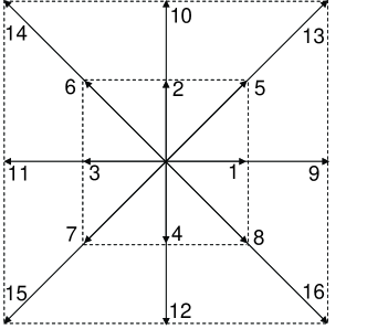
Figure 1: Schematics of $\mathbf{v}_{i}$ for the discrete velocity model.

We construct a two-dimensional MRT LB model based on a $16$-discrete-velocity model (see Fig. 1):

$$\left(v_{i1,}v_{i2}\right)=\left\{\begin{array}[]{cc}\mathbf{cyc}:\left(\pm 1,0\right),&\text{for }1\leq i\leq 4,\\ \left(\pm 1,\pm 1\right),&\text{for }5\leq i\leq 8,\\ \mathbf{cyc}:\left(\pm 2,0\right),&\text{for }9\leq i\leq 12,\\ \left(\pm 2,\pm 2\right),&\text{for }13\leq i\leq 16,\end{array}\right.$$

where cyc indicates the cyclic permutation.

The transformation matrix $\mathbf{M}$ is constructed according to the irreducible representation bases of SO(2) group, and it can be expressed as follows:

$$\mathbf{M}=(m_{1},m_{2},\cdots,m_{16})^{T}\text{,}$$

where

$$m_{1}=(1,1,1,1,1,1,1,1,1,1,1,1,1,1,1,1)\text{,}$$

$$m_{2}=(1,0,-1,0,1,-1,-1,1,2,0,-2,0,2,-2,-2,2)\text{,}$$

$$m_{3}=(0,1,0,-1,1,1,-1,-1,0,2,0,-2,2,2,-2,-2)\text{,}$$

$$m_{4}=(\frac{1}{2},\frac{1}{2},\frac{1}{2},\frac{1}{2},1,1,1,1,2,2,2,2,4,4,4,4)\text{,}$$

$$m_{5}=(1,-1,1,-1,0,0,0,0,4,-4,4,-4,0,0,0,0)\text{,}$$

$$m_{6}=(0,0,0,0,1,-1,1,-1,0,0,0,0,4,-4,4,-4)\text{,}$$

$$m_{7}=(\frac{1}{2},0,-\frac{1}{2},0,1,-1,-1,1,4,0,-4,0,8,-8,-8,8)\text{,}$$

$$m_{8}=(0,\frac{1}{2},0,-\frac{1}{2},1,1,-1,-1,0,4,0,-4,8,8,-8,-8)\text{,}$$

$$m_{9}=(1,0,-1,0,-2,2,2,-2,8,0,-8,0,-16,16,16,-16)\text{,}$$

$$m_{10}=(0,-1,0,1,2,2,-2,-2,0,-8,0,8,16,16,-16,-16)\text{,}$$

$$m_{11}=(\frac{1}{4},\frac{1}{4},\frac{1}{4},\frac{1}{4},1,1,1,1,4,4,4,4,16,16,16,16)\text{,}$$

$$m_{12}=(1,1,1,1,-4,-4,-4,-4,16,16,16,16,-64,-64,-64,-64)\text{,}$$

$$m_{13}=(1,-1,1,-1,0,0,0,0,16,-16,16,-16,0,0,0,0)\text{,}$$

$$m_{14}=(0,0,0,0,2,-2,2,-2,0,0,0,0,32,-32,32,-32)\text{,}$$

$$m_{15}=(1,0,-1,0,-4,4,4,-4,32,0,-32,0,-128,128,128,-128)\text{,}$$

$$m_{16}=(0,-1,0,1,4,4,-4,-4,0,-32,0,32,128,128,-128,-128)\text{.}$$

For two-dimensional compressible models, we have four conserved moments, density $\rho$, momentums $j_{x}$, $j_{y}$, and energy $e$. They are denoted by $\hat{f}_{1}$, $\hat{f}_{2}$, $\hat{f}_{3}$ and $\hat{f}_{4}$, respectively. Specifically, $\hat{f}_{1}=\rho$, $\hat{f}_{2}=j_{x}$, $\hat{f}_{3}=j_{y}$, $\hat{f}_{4}=e=\rho(T+u^{2}/2)$. Using the Chapman-Enskog expansionDuShi ; McCracken ; 22 on the two sides of LB equation, the Navier-Stokes (NS) equations for compressible fluids can be derived. The equilibria of the nonconserved moments can be chosen as

$$\hat{f}_{5}^{eq}=(j_{x}^{2}-j_{y}^{2})/\rho,$$ (2a)

$$\hat{f}_{6}^{eq}=j_{x}j_{y}/\rho,$$ (2b)

$$\hat{f}_{7}^{eq}=(e+\rho RT)j_{x}/\rho,$$ (2c)

$$\hat{f}_{8}^{eq}=(e+\rho RT)j_{y}/\rho,$$ (2d)

$$\hat{f}_{9}^{eq}=(j_{x}^{2}-3j_{y}^{2})j_{x}/\rho^{2},$$ (2e)

$$\hat{f}_{10}^{eq}=(3j_{x}^{2}-j_{y}^{2})j_{y}/\rho^{2},$$ (2f)

$$\hat{f}_{11}^{eq}=2e^{2}/\rho-(j_{x}^{2}+j_{y}^{2})^{2}/4\rho^{3},$$ (2g)

$$\hat{f}_{13}^{eq}=(6\rho e-2j_{x}^{2}-2j_{y}^{2})(j_{x}^{2}-j_{y}^{2})/\rho^{3},$$ (2h)

$$\hat{f}_{14}^{eq}=(6\rho e-2j_{x}^{2}-2j_{y}^{2})j_{x}j_{y}/\rho^{3}\text{.}$$ (2i)

The recovered NS equations are as follows:

$$\frac{\partial\rho}{\partial t}+\frac{\partial j_{x}}{\partial x}+\frac{\partial j_{y}}{\partial y}=0,$$ (3a)

$$\frac{\partial j_{x}}{\partial t}+\frac{\partial}{\partial x}\left(j_{x}^{2}/\rho\right)+\frac{\partial}{\partial y}\left(j_{x}j_{y}/\rho\right)=-\frac{\partial P}{\partial x}+\frac{\partial}{\partial x}[\mu_{s}(\frac{\partial u_{x}}{\partial x}-\frac{\partial u_{y}}{\partial y})]+\frac{\partial}{\partial y}[\mu_{v}(\frac{\partial u_{y}}{\partial x}+\frac{\partial u_{x}}{\partial y})],$$ (3b)

$$\frac{\partial j_{y}}{\partial t}+\frac{\partial}{\partial x}\left(j_{x}j_{y}/\rho\right)+\frac{\partial}{\partial y}\left(j_{y}^{2}/\rho\right)=-\frac{\partial P}{\partial y}+\frac{\partial}{\partial x}[\mu_{v}(\frac{\partial u_{y}}{\partial x}+\frac{\partial u_{x}}{\partial y})]-\frac{\partial}{\partial y}[\mu_{s}(\frac{\partial u_{x}}{\partial x}-\frac{\partial u_{y}}{\partial y})],$$ (3c)

$$\frac{\partial e}{\partial t}+\frac{\partial}{\partial x}[(e+P)j_{x}/\rho]+\frac{\partial}{\partial y}[(e+P)j_{y}/\rho]$$ (3d)

$$= \frac{\partial}{\partial x}[\lambda_{1}(R\frac{\partial T}{\partial x}+\frac{1}{2}(u_{y}\frac{\partial u_{y}}{\partial x}+u_{x}\frac{\partial u_{x}}{\partial x}-u_{x}\frac{\partial u_{y}}{\partial y}+u_{y}\frac{\partial u_{x}}{\partial y}))]$$

$$+\frac{\partial}{\partial y}[\lambda_{2}(R\frac{\partial T}{\partial y}+\frac{1}{2}(u_{x}\frac{\partial u_{x}}{\partial y}-u_{y}\frac{\partial u_{x}}{\partial x}+u_{x}\frac{\partial u_{y}}{\partial x}+u_{y}\frac{\partial u_{y}}{\partial y}))],$$

where $$\mu_{s}= \rho RT/s_{5} \mu_{v}= \rho RT/s_{6} \lambda_{1}=2\rho RT/s_{7} \lambda_{2}=2\rho RT/s_{8}$$ , , , .

When $\mu_{s}=$ $\mu_{v}=\mu$, $\lambda_{1}=\lambda_{2}=\lambda$, the above NS equations reduce to

$$\frac{\partial\rho}{\partial t}+\frac{\partial j_{\alpha}}{\partial x_{\alpha}}=0,$$ (4a)

$$\frac{\partial j_{\alpha}}{\partial t}+\frac{\partial\left(j_{\alpha}j_{\beta}/\rho\right)}{\partial x_{\beta}}=-\frac{\partial P}{\partial x_{\alpha}}+\frac{\partial}{\partial x_{\beta}}[\mu(\frac{\partial u_{\alpha}}{\partial x_{\beta}}+\frac{\partial u_{\beta}}{\partial x_{\alpha}}-\frac{\partial u_{\chi}}{\partial x_{\chi}}\delta_{\alpha\beta})],$$ (4b)

$$\frac{\partial e}{\partial t}+\frac{\partial}{\partial x_{\alpha}}[(e+P)j_{\alpha}/\rho]=\frac{\partial}{\partial x_{\alpha}}[\lambda(R\frac{\partial T}{\partial x_{\alpha}}+\frac{1}{2}u_{\beta}(\frac{\partial u_{\alpha}}{\partial x_{\beta}}+\frac{\partial u_{\beta}}{\partial x_{\alpha}}-\frac{\partial u_{\chi}}{\partial x_{\chi}}\delta_{\alpha\beta}))]\text{.}$$ (4c)

It should be pointed out that, the viscous coefficient in the energy equation (4c) is not consistent with that in the momentum equation (4b). Motivated by the idea of Guo et al. guo2 , the collision operators of the moments related to the energy flux are modified:

$$\hat{\mathbf{S}}_{77}(\hat{f}_{7}-\hat{f}_{7}^{eq})\Rightarrow\hat{\mathbf{S}}_{77}(\hat{f}_{7}-\hat{f}_{7}^{eq})+(s_{7}/s_{5}-1)\rho Tu_{x}(\frac{\partial u_{x}}{\partial x}-\frac{\partial u_{y}}{\partial y})+(s_{7}/s_{6}-1)\rho Tu_{y}(\frac{\partial u_{y}}{\partial x}+\frac{\partial u_{x}}{\partial y})\text{,}$$

$$\hat{\mathbf{S}}_{88}(\hat{f}_{8}-\hat{f}_{8}^{eq})\Rightarrow\hat{\mathbf{S}}_{88}(\hat{f}_{8}-\hat{f}_{8}^{eq})+(s_{8}/s_{6}-1)\rho Tu_{x}(\frac{\partial u_{y}}{\partial x}+\frac{\partial u_{x}}{\partial y})+(s_{8}/s_{5}-1)\rho Tu_{y}(\frac{\partial u_{x}}{\partial x}-\frac{\partial u_{y}}{\partial y})\text{.}$$

With this modification, we are able to get the following thermohydrodynamic equations:

$$\frac{\partial\rho}{\partial t}+\frac{\partial j_{\alpha}}{\partial x_{\alpha}}=0,$$ (5a)

$$\frac{\partial j_{\alpha}}{\partial t}+\frac{\partial\left(j_{\alpha}j_{\beta}/\rho\right)}{\partial x_{\beta}}=-\frac{\partial P}{\partial x_{\alpha}}+\frac{\partial}{\partial x_{\beta}}[\mu(\frac{\partial u_{\alpha}}{\partial x_{\beta}}+\frac{\partial u_{\beta}}{\partial x_{\alpha}}-\frac{\partial u_{\chi}}{\partial x_{\chi}}\delta_{\alpha\beta})],$$ (5b)

$$\frac{\partial e}{\partial t}+\frac{\partial}{\partial x_{\alpha}}[(e+P)j_{\alpha}/\rho]=\frac{\partial}{\partial x_{\alpha}}[\lambda R\frac{\partial T}{\partial x_{\alpha}}+\mu u_{\beta}(\frac{\partial u_{\alpha}}{\partial x_{\beta}}+\frac{\partial u_{\beta}}{\partial x_{\alpha}}-\frac{\partial u_{\chi}}{\partial x_{\chi}}\delta_{\alpha\beta})]\text{.}$$ (5c)

This modification method is also suitable for our previous MRT modelschenepl ; chenpla . The definitions of $\hat{f}_{12}^{eq}$, $\hat{f}_{15}^{eq}$, $\hat{f}_{16}^{eq}$ have no effect on macroscopic equations, so the choices of the three moments are flexible. Now we give three different and typical formations: $\hat{f}_{12}^{eq}=\hat{f}_{15}^{eq}=\hat{f}_{16}^{eq}=0$ (version 1); $\hat{f}_{12}^{eq}=0$,$\ \hat{f}_{15}^{eq}=\rho u_{x}(-4+10T+5u_{x}^{2}-5u_{y}^{2})$, $\hat{f}_{16}^{eq}=\rho u_{y}(4-10T+5u_{x}^{2}-5u_{y}^{2})$ (version 2); $\hat{f}_{12}^{eq}=M_{12i}f_{i}^{\max}$, $\hat{f}_{15}^{eq}=M_{15i}f_{i}^{\max}$, $\hat{f}_{16}^{eq}=M_{16i}f_{i}^{\max}$, $f_{i}^{\max}=\rho/(2\pi T)\exp(-(v_{i\alpha}-u_{\alpha})^{2}/(2T))$ (version 3). In the second version, the MRT model reduces to the usual lattice BGK model in ref.Chen1994 which uses a higher-order velocity expansion for Maxwellian-type equilibrium distribution, if all the relaxation parameters are set to be a single relaxation frequency $s$, namely $\mathbf{S}=s\mathbf{I}$.

III Stability Analysis

In this section, the von Neumann stability analysischenpla on the new MRT LB model is performed. In the stability analysis, we write the solution of FD LB equation in the form of Fourier series. If all the eigenvalues of the coefficient matrix are less than 1, the algorithm is stable. Coefficient matrix $G_{ij}$ of the unmodified model can be expressed as follows,

$$G_{ij} =\delta_{ij}-\frac{v_{i\alpha}\Delta t}{2\Delta x_{\alpha}}(e^{\mathbf{i}k_{\alpha}\Delta x_{\alpha}}-e^{-\mathbf{i}k_{\alpha}\Delta x_{\alpha}})\delta_{ij}+\frac{1}{2}(\frac{v_{i\alpha}\Delta t}{\Delta x_{\alpha}})^{2}(e^{\mathbf{i}k_{\alpha}\Delta x_{\alpha}}-2$$

$$+e^{-\mathbf{i}k_{\alpha}\Delta x_{\alpha}})\delta_{ij}-\Delta t\mathbf{M}_{il}^{-1}\hat{\mathbf{S}}_{lk}(\frac{\partial\hat{f}_{k}}{\partial f_{j}}-\frac{\partial\hat{f}_{k}^{eq}}{\partial f_{j}})\text{,}$$ (6)

where

$$\hat{f}_{k}=\mathbf{M}_{kp}f_{p}\text{,}$$

$$\frac{\partial\hat{f}_{k}^{eq}}{\partial f_{j}}=\frac{\partial\hat{f}_{k}^{eq}}{\partial\rho}\frac{\partial\rho}{\partial f_{j}}+\frac{\partial\hat{f}_{k}^{eq}}{\partial T}\frac{\partial T}{\partial f_{j}}+\frac{\partial\hat{f}_{k}^{eq}}{\partial u_{\alpha}}\frac{\partial u_{\alpha}}{\partial f_{j}}\text{.}$$ (7)

Because of the modification of the collision operators, the coefficient matrix $G_{ij}$ corresponding to energy flux should be replaced by

$$G_{ij} =\delta_{ij}-\frac{v_{i\alpha}\Delta t}{2\Delta x_{\alpha}}(e^{\mathbf{i}k_{\alpha}\Delta x_{\alpha}}-e^{-\mathbf{i}k_{\alpha}\Delta x_{\alpha}})\delta_{ij}+\frac{1}{2}(\frac{v_{i\alpha}\Delta t}{\Delta x_{\alpha}})^{2}(e^{\mathbf{i}k_{\alpha}\Delta x_{\alpha}}-2$$

$$+e^{-\mathbf{i}k_{\alpha}\Delta x_{\alpha}})\delta_{ij}-\Delta t\mathbf{M}_{i7}^{-1}\hat{\{\mathbf{S}}_{77}(\frac{\partial\hat{f}_{7}}{\partial f_{j}}-\frac{\partial\hat{f}_{7}^{eq}}{\partial f_{j}})+\frac{\partial}{\partial f_{j}}[(s_{7}/s_{5}-1)\rho Tu_{x}(\frac{\partial u_{x}}{\partial x}-\frac{\partial u_{y}}{\partial y})]$$

$$+\frac{\partial}{\partial f_{j}}[(s_{7}/s_{6}-1)\rho Tu_{y}(\frac{\partial u_{y}}{\partial x}+\frac{\partial u_{x}}{\partial y})]\}\text{,}$$ (8)

and

$$G_{ij} =\delta_{ij}-\frac{v_{i\alpha}\Delta t}{2\Delta x_{\alpha}}(e^{\mathbf{i}k_{\alpha}\Delta x_{\alpha}}-e^{-\mathbf{i}k_{\alpha}\Delta x_{\alpha}})\delta_{ij}+\frac{1}{2}(\frac{v_{i\alpha}\Delta t}{\Delta x_{\alpha}})^{2}(e^{\mathbf{i}k_{\alpha}\Delta x_{\alpha}}-2$$

$$+e^{-\mathbf{i}k_{\alpha}\Delta x_{\alpha}})\delta_{ij}-\Delta t\mathbf{M}_{i8}^{-1}\hat{\{\mathbf{S}}_{88}(\frac{\partial\hat{f}_{8}}{\partial f_{j}}-\frac{\partial\hat{f}_{8}^{eq}}{\partial f_{j}})+\frac{\partial}{\partial f_{j}}[(s_{8}/s_{6}-1)\rho Tu_{x}(\frac{\partial u_{y}}{\partial x}+\frac{\partial u_{x}}{\partial y})]$$

$$+\frac{\partial}{\partial f_{j}}[(s_{8}/s_{5}-1)\rho Tu_{y}(\frac{\partial u_{x}}{\partial x}-\frac{\partial u_{y}}{\partial y})]\}\text{.}$$ (9)

We conduct a quantitative analysis using the software, Mathematica. In Fig.2 we show some stability comparisons for the new MRT model, its SRT counterpart and our previous model in refs.chenepl ; chenpla . The abscissa is for $kdx$, and the vertical axis is for $|\omega|_{max}$ which is the largest eigenvalue of coefficient matrix $G_{ij}$. Grid sizes are $dx=dy=10^{-3}$, and time step is $dt=10^{-5}$, the relaxation frequency in SRT is $s=10^{5}$. The other parameters in stability analysis are chosen as follows: (a), $(\rho,u_{1},u_{2},T)$ = $(2.0,2.0,0.0,2.0)$, the collision parameters in MRT are $s_{i}=10^{5},i=1,\cdots,16$, the Mach number is 1 ($Ma=u/\sqrt{2T}=2/2$); (b), $(\rho,u_{1},u_{2},T)$ = $(2.0,6.0,0.0,2.0)$, the collision parameters in the three versions are $s_{9}=10^{3}$, those in modelchenepl are $s_{10}=5\times 10^{4}$, $s_{11}=2\times 10^{4}$, $s_{13}=1.5\times 10^{4}$, and those in chenpla are $s_{9}=8\times 10^{3}$, $s_{13}=7\times 10^{4}$, $s_{14}=5\times 10^{4}$, the others are $10^{5}$, and the Mach number is 3.0; (c), $(\rho,u_{1},u_{2},T)$ = $(2.0,10.0,0.0,2.0)$, the collision parameters in the three versions are $s_{9}=1.2\times 10^{4}$, $s_{13}=10^{2}$, $s_{14}=5\times 10^{4}$, $s_{15}=1.5\times 10^{3}$, those in modelchenepl are $s_{13}=1.5\times 10^{4}$, and those in modelchenpla are $s_{9}=2\times 10^{3}$, $s_{13}=6.1\times 10^{4}$, $s_{14}=s_{15}=3\times 10^{4}$, the others are $10^{5}$, and the Mach number is 5; (d), $(\rho,u_{1},u_{2},T)$ = $(2.0,12.0,0.0,2.0)$, the collision parameters in the three versions are $s_{9}=10^{4}$, $s_{13}=10^{2}$, $s_{14}=6\times 10^{4}$, $s_{15}=1.5\times 10^{3}$, and those in modelchenepl are $s_{11}=2\times 10^{4}$, $s_{13}=1.5\times 10^{4}$, and those in chenpla are $s_{9}=10^{3}$, $s_{13}=5\times 10^{3}$, $s_{14}=s_{15}=3\times 10^{4}$, the others are $10^{5}$, and the Mach number is 6. In case (a), the MRT and SRT have the same stability; with the increase of Mach number (case (b) and (c)), the MRT models are stable, while the SRT version is not; if further increases the Mach number, MRT models also encounter instability problem (case (d)). It is clear that, by choosing appropriate collision parameters, the stability of MRT can be much better than the SRT. Three versions of the new MRT model do not show large differences in numerical stability.

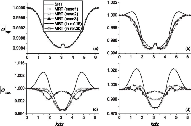
Figure 2: Stability comparison for the new MRT model and its SRT counterpart.

IV Numerical Simulations

In this section, we study the following problems using the modified MRT LB model: Couette flow, One-dimensional Riemann problem, and Richtmyer-Meshkov instability. We work in a frame where the constant $R=1$.

IV.1 Unshocked compressible fluids

Here we conduct a series of numerical simulations of Couette flow. The aims of simulation of Couette flow are twofold. At first, we prove the Maxwellian property of the discrete equilibrium functions. Consider a viscous fluid flow between two parallel flat plates, moving in the opposite directions, $U_{wr}=-U_{wl}=0.2$, where subscripts $wr$ and $wl$ indicate the walls in the right and left sides. The initial state of the fluid is $\rho=1$, $T=1$, $U=0$. The temperatures of walls are $T_{wr}=T_{wl}=1$. Near the walls, we adopt the diffuse reflection boundary conditions proposed by Sofonea, et aldiffuse . In the other two boundaries the periodic boundary condition is adopted. In the diffuse reflection boundary, the particles leaving the wall are assumed to follow the Maxwellian distribution. Following the discretization of the velocity space, in the FD LB model the Maxwellian distribution function is replaced by the equilibrium distribution function.

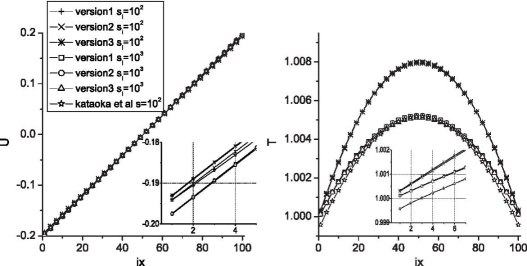
Figure 3: Slip velocity and temperature jump simulated with the three versions and the model proposed by Kataoka, et al.

Fig. 3 shows the velocity and temperature profiles simulated with the three versions of this proposed model and the model proposed by Kataoka, et alKataoka . The abscissa $ix$ is the index of lattice node in the $x$- directions, and the vertical axes are velocity $u$ and temperature $T$, respectively. The parameters are $dx=dy=0.01$, $dt=10^{-4}$, $NX\times NY=100\times 5$. The diffuse reflection boundary conditions work well with our model, the slip velocity and temperature jump near the walls are clearly seen, and increase with Knudsen number. While it fails to work for the model by Kataoka et al, because the temperature near the wall is lower than the wall temperature, which is contrary to physical idea. In Couette flow the fluid at the walls should have a higher temperature than the walls themselves, because of the heat generated by the viscous flow. We think this contradiction is caused from the equilibrium distribution function in their model which is not a Taylor expansion of the Maxwellian. So it departs from the basic assumption of diffuse reflection boundary. None of the three versions violates the basic assumption and destroys the Maxwellian property of the discrete equilibrium functions.

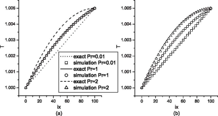
Figure 4: Effects of heat conductivity on temperature profiles of Couette flow. (a) corresponds to the unmodified model(version 1), and (b) corresponds to the modified model. $Pr=0.01$, $Pr=1$ and $Pr=2$ correspond to $s_{7}=s_{8}=10$, $s_{7}=s_{8}=10^{3}$, and $s_{7}=s_{8}=2\times 10^{3}$, respectively (other collision parameters are $10^{3}$).

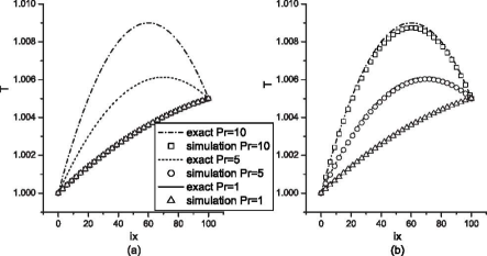
Figure 5: Effects of viscosity on temperature profiles of Couette flow. (a) corresponds to the unmodified model(version 1), and (b) corresponds to the modified model. $Pr=10$, $Pr=5$ and $Pr=1$ correspond to $s_{5}=s_{6}=10^{2}$, $s_{5}=s_{6}=2\times 10^{2}$, and $s_{5}=s_{6}=10^{3}$, respectively (other collision parameters are $10^{3}$).

Secondly, we will compare the ability of the unmodified model and the modified model for the unshocked compressible fluids. In the simulation, the left wall is fixed and the right wall moves at speed $U=0.1$. The simulation results are compared with the analytical solution:

$$T=T_{1}+(T_{2}-T_{1})\frac{x}{H}+\frac{\mu}{2\lambda}U^{2}\frac{x}{H}(1-\frac{x}{H})\text{,}$$

where $T_{1}$ and $T_{2}$ are the left and right wall’s temperatures ($T_{1}=1$, $T_{2}=1.005$), $H$ is the width of the channel. Other parameters remain unchanged. Periodic boundary conditions are applied to the bottom and top boundaries, and the left and right walls adopt the nonequilibrium extrapolation method. Fig. 4 and Fig. 5 show the temperature profiles of Couette flow simulated with the unmodified model (version 1) and its modified version. In Fig. 4, we fix viscosity coefficient $s_{5}=s_{6}=10^{3}$, and change the thermal conductivity $s_{7}=s_{8}$ from $10$ to $2\times 10^{3}$. On the contrary, we fix thermal conductivity $s_{7}=s_{8}=10^{3}$, and change the viscosity $s_{5}=s_{6}$ from $10^{2}$ to $10^{3}$ in Fig. 5. (a) corresponds to the unmodified model (version 1), and (b) corresponds to the modified model. It is clearly shown that the simulation results of modified model are in agreement with the analytical solutions, and the Prandtl number effects on unshocked compressible fluids are successfully captured by the modified model, but not by the unmodified model.

IV.2 Shocked compressible fluids

(a) Riemann problem

Here we construct a high Mach number shock tube problem with the initial condition,

$$\left\{\begin{array}[]{cc}(\rho,u_{1},u_{2},T)|_{L}=(5.0,45.0,0.0,10.0),&x\leq 0\text{.}\\ (\rho,u_{1},u_{2},T)|_{R}=(6.0,-20.0,0.0,5.0),&x>0\text{.}\end{array}\right.$$ (10)

The Mach number of the left side is $10.1$ ($Ma=u/\sqrt{2T}=45/\sqrt{20}$), and the right is $6.3$ ($Ma=u/\sqrt{2T}=20/\sqrt{10}$). Figure 6 shows the comparison of LB results and exact solutions at $t=0.018$, where the parameters are $dx=dy=0.003$, $dt=10^{-5}$, $s_{5}=s_{6}=1.5\times 10^{4}$, other values of $s$ are $10^{5}$. Squares correspond to simulation results with the unmodified model (version 1), the circle symbols correspond to the modified MRT simulation results, and solid lines represent the exact solutions, respectively. It can be seen that the simulations of the two MRT models do not show large differences. For shocked compressible flows, there exist a fast procedure and a slow one. The shock dynamic procedure is fast, while that of heat conduction is slow. In such a case, from the view of macroscopic description, the terms related to viscosity and heat conductivity may be neglected. So, terms related to viscosity and heat conductivity in Eqs.(3) and (5) are all small terms and make negligible effects. That is the reason why the unmodified model works also well in such cases.

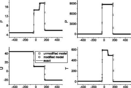
Figure 6: LB results and exact solutions for shock tube problem at time $t=0.018$. $\rho$: density, $P$: pressure, $U$: the $x-$ component of velocity, $T$: temperature.

(b) Richtmyer-Meshkov instability

The Richtmyer-Meshkov (RM) instabilityRichtmyer ; Meshkov is a fundamental fluid instability that develops when an incident shock wave collides with an interface between two fluids with different densities. This instability is involved in numerous physical processes, such as inertial confined fusion, supersonic and hypersonic combustion, supernova explosion, and so on. RM instability has attracted considerable attention for several decades because of its important theoretical and practical significance. To the best of our knowledge, the research of RM instability by LB method is still very limited. In this paper, we study the thermal conductivity and viscosity effects on RM instability with the MRT LB method.

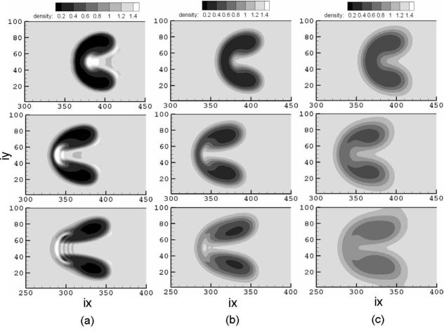
Figure 7: Snapshots of shock wave reaction on single bubble. The left column (a) corresponds to $s_{5}=s_{6}=10^{4},s_{7}=s_{8}=10^{5}$, the middle column (b) corresponds to $s_{5}=s_{6}=10^{4},s_{7}=s_{8}=10^{4}$, and the right column (c) corresponds to $s_{5}=s_{6}=10^{4},s_{7}=s_{8}=10^{3}$. From black to white the grey level corresponds to the increase of density.

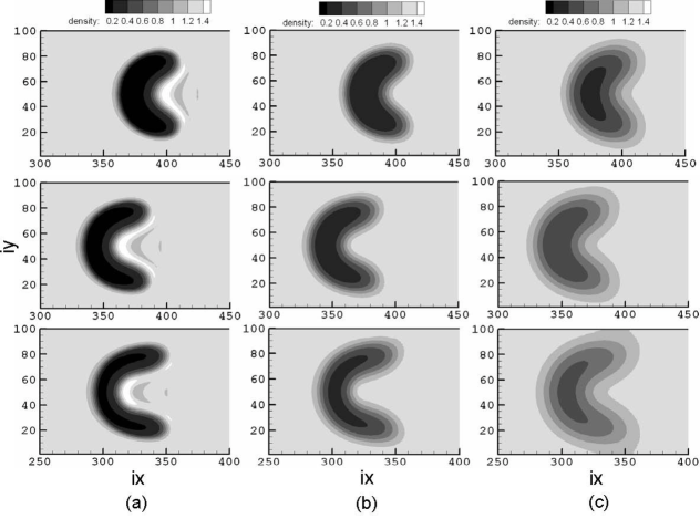
Figure 8: Snapshots of shock wave reaction on single bubble. The left column (a) corresponds to $s_{5}=s_{6}=10^{3},s_{7}=s_{8}=10^{5}$, the middle column (b) corresponds to $s_{5}=s_{6}=10^{3},s_{7}=s_{8}=10^{4}$, and the right column (c) corresponds to $s_{5}=s_{6}=10^{3},s_{7}=s_{8}=10^{3}$. From black to white the grey level corresponds to the increase of density.

The investigation of the interaction of a planar shock with an isolated gas bubble is of special significance in the study of RM instability, because the interface of gas bubble has typical three dimensional characteristic and large initial distortion. It helps to understand the mechanism of RM instability process. The problem we simulated is as follows: A planar shock wave with the Mach number $1.22$ ($D=1.725$), traveling from the right side, impinges on a cylindrical bubble. The initial macroscopic quantities are as follows:

$$\left(\rho,u_{1},u_{2},p\right)\mid_{x,y,0}=\left\{\begin{array}[]{cc}\left(1,0,0,1\right),&\mathbf{pre-shock}\text{{,}}\\ \left(1.28,-0.3774,0,1.6512\right),&\mathbf{post-shock}\text{{,}}\\ \left(0.1358,0,0,1\right),&\mathbf{bubble}\text{{,}}\end{array}\right.$$ (11)

The domain of computation is a rectangle $Nx\times Ny=600\times 100$, $Nx$ and $Ny$ are the numbers of lattice node in the $x$- and $y$- directions. Initially, the bubble is at the position (450,50), the post-shock domain is $\left[501,600\right]\times\left[0,100\right]$. In the simulations, the right side adopts the initial values of post-shock flow, the extrapolation technique is applied at the left boundary, and reflection conditions are imposed on the other two surfaces.

In Figures 7 and 8, we show some simulation results with different configurations. The abscissa is for $ix$, and the vertical axis is for $iy$, where $ix$ and $iy$ are the indexes of lattice node in the $x$- and $y$- directions. From top to bottom, the three rows show the density contours at times $t=0.5$, $0.7$, $1$, respectively. The common parameters are $dx=dy=0.003$, $dt=10^{-5}$. The collision parameters in Fig. 7(a) are $s_{5}=s_{6}=10^{4}$, $s_{7}=s_{8}=10^{5}$, those in Fig. 7(b) are $s_{5}=s_{6}=10^{4}$, $s_{7}=s_{8}=10^{4}$, and those in Fig. 7(c) are $s_{5}=s_{6}=10^{4}$, $s_{7}=s_{8}=10^{3}$, $10^{5}$ for the others. The collision parameters in Fig. 8(a) are $s_{5}=s_{6}=10^{3}$, $s_{7}=s_{8}=10^{5}$, those in Fig. 8(b) are $s_{5}=s_{6}=10^{3}$, $s_{7}=s_{8}=10^{4}$, and those in Fig. 8(c) are $s_{5}=s_{6}=10^{3}$, $s_{7}=s_{8}=10^{3}$, $10^{5}$ for the others. Fig. 7 and Fig. 8 show that when the viscosity is constant, the small thermal conductivity is beneficial to the development of RM instability. Comparing Fig. 7 with Fig. 8, we find when the thermal conductivity is constant, the small viscosity is beneficial to the development of RM instability. The thermal conductivity and viscosity have inhibition effects on the development of RM instability. Both the unmodified model and the modified model get the same results.

V Conclusions

We propose a MRT Lattice Boltzmann model which works not only for the shocked compressible fluids but also for the unshocked compressible fluids. In the new model, a key step is the modification of the collision operators of energy flux so that viscous coefficient in momentum equation and that in energy equation are consistent no matter if the system is shocked or not. The unnecessity of the modification for systems under strong shock is analyzed. The new model is validated by some well-known benchmark tests, including (i) thermal Couette flow, (ii) Riemann problem, (iii) Richtmyer-Meshkov instability. The first system is unshocked and the latter two are shocked. In all the three systems, the Prandtl numbers effects are checked. Satisfying agreements are obtained between the new model results and analytical ones or other numerical results. Our previous modelschenepl ; chenpla can be revised in the same way to simulate unshocked compressible flows.

References

- (1) S. Succi, The Lattice Boltzmann Equation for Fluid Dynamics and Beyond, Oxford University Press, New York (2001).
- (2) R. Benzi, S. Succi, and M. Vergassola, Phys. Rep. 222 (1992) 145.
- (3) Aiguo Xu, G. Gonnella, and A. Lamura, Phys. Rev. E 67 (2003) 056105; Phys. Rev. E 74 (2006) 011505; Physica A 331 (2004) 10; Physica A 344 (2004) 750; Physica A 362 (2006) 42.
- (4) F. Tosi, S. Ubertini, S. Succi, H. Chen, and I. V. Karlin, Math. Comput. Simul. 72 (2006) 227.
- (5) S. Ansumali, I.V. Karlin, J. Stat. Phys. 107 (2002) 291.
- (6) V. Sofonea, A. Lamura, G. Gonnella, and A. Cristea, Phys. Rev. E 70 (2004) 046702.
- (7) X. F. Pan, Aiguo Xu, and Guangcai Zhang, S. Jiang, Int. J. Mod. Phys. C 18 (2007) 1747; Y. Gan, Aiguo Xu, Guangcai Zhang, X. Yu, and Y. Li, Physica A 387 (2008) 1721.
- (8) R. A. Brownlee, A. N. Gorban, J. Levesley, Phys. Rev. E 75 (2007) 036711.
- (9) F. J. Higuera, S. Succi, and R. Benzi, Europhys. Lett. 9 (1989) 345. F. J. Higuera, J. Jimenez, Europhys. Lett. 9 (1989) 662.
- (10) D. d’Humières, Generalized lattice-Boltzmann equations, in Rarefied Gas Dynamics: Theory and Simulations, edited by B. D. Shizgal and D. P Weaver, Progress in Astronautics and Aeronautics, Vol. 159(AIAA Press, Washington, DC, 1992), pp450-458.
- (11) R. Adhikari, S. Succi, Phys. Rev. E 78 (2008) 066701.
- (12) P. Lallemand, L. S. Luo, Phys. Rev. E 61 (2000) 6546.
- (13) R. Du, B. Shi, and X. Chen, Phys. Lett. A 359 (2006) 564.
- (14) M. E. McCracken, J. Abraham, Phys. Rev. E 71 (2005) 036701.
- (15) L. Zheng, Z.L. Guo, B.C. Shi, and C.G. Zheng, Phys. Rev. E 81 (2010) 016706.
- (16) P. Lallemand, L. S. Luo, Phys. Rev. E 68 (2003) 036706.
- (17) L. Zheng, B.C. Shi, Z.L. Guo, Phys. Rev. E 78 (2008) 026705.
- (18) A. Mezrhab, M. A. Moussaouia, M. Jami, H. Naji, and M. Bouzidi, Physics Letters A 374 (2010) 3499.
- (19) F. Chen, Aiguo Xu, G. C. Zhang, Y. J. Li, and S. Succi, Europhys. Lett. 90 (2010) 54003.
- (20) F. Chen, Aiguo Xu, G. C. Zhang, Y. J. Li, Physics Letters A 375 (2011) 2129.
- (21) S. Chapman and T.G. Cowling, The mathematical theory of non-uniform gases, Cambridge University Press, London (1970).
- (22) Y. Chen, H. Ohashi, and M. Akiyama, Phys. Rev. E 50 (1994) 2776.
- (23) V. Sofonea, and R. F. Sekerka, Phys. Rev. E 71 (2005) 066709.
- (24) T. Kataoka, M. Tsutahara, Phys. Rev. E 69 (2004) 035701(R).
- (25) R. D. Richtmyer, Commun. Pure Appl. Maths. 8 (1960) 297.
- (26) E. E. Meshkov, Sov. Fluid Dyn. 4 (1969) 101.