Superfluid density of an open dissipative condensate

Abstract

I calculate the superfluid density of a non-equilibrium steady state condensate of particles with finite lifetime. Despite the absence of a simple Landau critical velocity, a superfluid response survives, but dissipation reduces the superfluid fraction. I also suggest an idea for how the superfluid density of an example of such a system, i.e. microcavity polaritons, might be measured.

The observation of superfluidity is one of the most compelling signatures of quantum coherence in systems such as Helium and cold atomic gases Leggett (2006). Recently, there has been much activity exploring condensation of mixed matter-light excitations, i.e. semiconductor microcavity polaritons (see Deng et al. (2010) for a review) as well as recent experiments on photons in dye filled cavities Klaers et al. (2010). Microcavity polaritons consist of superpositions of excitons confined in quantum wells, and photons confined in semiconductor microcavities. Because of the photonic component of these particles, they have a finite lifetime, and so any condensate will be a non-equilibrium steady state, where loss is balanced by injection of new particles. As well as these matter-light systems, recent experiments on continuous loading of cold atoms into traps Falkenau et al. suggest that similar questions of superfluid properties in non-equilibrium steady states may soon be accessible in cold atoms.

Finite particle lifetime prompts questions about the meaning of superfluidity when the particles involved in the condensate are continually being replaced. To see why such questions arise, one may observe that finite particle lifetime changes the excitation spectrum from the linearly dispersing Bogoliubov sound mode to a diffusive mode Szymańska et al. (2006); Wouters and Carusotto (2006), $\xi(k)=-i\sigma+\sqrt{c^{2}k^{2}-\sigma^{2}}$. The form of the spectrum of long wavelength modes is commonly invoked in explaining the existence of superfluidity, i.e. if the low energy excitations are linearly dispersing Bogoliubov sound modes, then there exists a critical velocity, such that for a fluid flowing below this velocity, it is not energetically favorable to create quasiparticle excitations, and thus the flowing superfluid remains stable Leggett (2006). If one naively defines a critical velocity by the dispersion of the real part of $\omega(k)$, one finds that for the non-equilibrium spectrum, such a critical velocity vanishes. As has been pointed out elsewhere Wouters and Carusotto (2010); Wouters and Savona (2010), a more careful argument regarding the response to a static defect indicates that there may still be a particular velocity at which there is a sharp onset of drag. Nonetheless, the above illustrates why non-equilibrium condensates require one to re-examine questions of superfluidity.

Experimentally, aspects of superfluid behavior have been studied in microcavity polariton systems, and features such as quantized vortices Lagoudakis et al. (2008), suppression of scattering off disorder Amo et al. (2009a); *Amo2009a and metastability of induced vortices Sanvitto et al. (2010) have been observed. While these various experiments show that aspects of superfluid behavior can be seen in such non-equilibrium condensates, they leave open an important question, namely what is the superfluid fraction. Even in superfluid Helium, at non-zero temperatures there are drag forces due to the normal fluid component. However, the normal and superfluid components can be clearly distinguished by their response to a slow rotation Leggett (2006): At low angular velocities, the superfluid cannot rotate, so only the normal component rotates, thus reducing the effective moment of inertia. Determining the normal and superfluid densities thus gives a fuller description of the superfluid properties of a system than does a binary distinction between superfluid and non-superfluid systems. As such, the aim of this letter is to discuss the normal and superfluid densities of an open dissipative condensate, and to suggest how this might be explored in the microcavity polariton systems.

The same superfluid density as introduced above can be found from the current-current response function $\chi_{ij}(q)$. This response function gives the particle current $J_{i}(q)=\sum_{k}\psi^{\dagger}_{k+q}\gamma_{i}(2\boldsymbol{k}+\boldsymbol{q})\psi_{k}$ (where the current vertex $\gamma_{i}(\boldsymbol{k})=k_{i}/2m$ and $\hbar=1$ throughout) due to a perturbation $H\to H-\sum_{q}f_{i}(q)J_{i}(q)$, i.e. $J_{i}(q)=\chi_{ij}(q)f_{j}(q)$. In an isotropic system, one may then define $\rho_{s},\rho_{n}$ as Leggett (2006)

$$m\chi_{ij}(q\to 0,\omega=0)=\rho_{s}\frac{q_{i}q_{j}}{q^{2}}+\rho_{n}\delta_{ij}.$$ (1)

The superfluid component picks out and responds only to the irrotational (non-transverse) part of the applied force. The advantage of this approach is that it allows an explicit calculation for the open dissipative system, using the Schwinger-Keldysh approach for non-equilibrium systems (see e.g. Altland and Simons (2010); *kamenev05).

In the following, I will consider the simplest model of a weakly interacting dilute Bose gas:

$$H=\sum_{k}\epsilon_{k}\psi^{\dagger}_{k}\psi^{\vphantom{\dagger}}_{k}+\sum_{k,k^{\prime},q}\frac{U}{2}\psi^{\dagger}_{k+q}\psi^{\dagger}_{k^{\prime}-q}\psi^{\vphantom{\dagger}}_{k^{\prime}}\psi^{\vphantom{\dagger}}_{k}$$ (2)

where $\epsilon_{k}=k^{2}/2m$. In addition, one must include pump and decay processes such that the bare inverse retarded Green’s function $[D^{R}_{(0)}]^{-1}=\omega-\epsilon_{k}+i\kappa-ip(\omega)$ where the pump has the form $p(\omega)=\gamma-\eta\omega$ and $\kappa$ describes decay. This form of pumping is motivated by recent works by Wouters and Carusotto (2010) (as well as related models Wouters and Savona ), and simplifies the calculation of $\chi_{ij}$ compared to models with density-dependent pump processes. When condensed, such a model has the diffusive spectrum $\zeta(k)=-i\sigma+\sqrt{c^{2}k^{2}-\sigma^{2}}$ with $\sigma=\eta\mu/(1+\eta^{2}),c=\sqrt{\mu/[m(1+\eta^{2})]}$. Thus, finding a non-zero superfluid density in such a model addresses how the diffusive spectrum affects superfluidity.

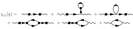
Figure 1: Types of Feynman diagram required for the response function to one-loop order. Straight lines indicate non-condensate excitations. Filled symbols involve the condensate, arising from either interactions (circles) or coupling to currents (squares). Wavy lines indicate source fields coupling to the current vertices.

To correctly find the superfluid response function Griffin (1994) requires vertex corrections in the response function. In equilibrium, this can be avoided by using sum rules that result from conservation of density, however with finite particle lifetimes, this is not necessarily a-priori justified. I will postpone until later the discussion of how the vertex corrections are to be determined and next summarize the physical reason that a superfluid density can survive.

Fig. 1 illustrates the classes of Feynman diagram (including vertex corrections) that result at one loop order. The first five diagrams contribute to the superfluid density, while the last gives the normal density. This can be seen by noting that the first five diagrams all have the current vertex scatter a particle out of the condensate, and thus involve a factor $\gamma_{i}(\boldsymbol{q})\propto q_{i}$, hence they all contribute to $\chi_{ij}\propto q_{i}q_{j}$. In order that the superfluid density does not vanish, it is crucial that the fluctuation propagator $D^{R}(\boldsymbol{q},\omega=0)$ that also appears in these five diagrams behave as $1/q^{2}$ at $q\to 0$ so that overall $\chi_{ij}\propto q_{i}q_{j}/q^{2}$ remains finite. The existence of superfluid density therefore depends on how the denominator of the Green’s function behaves.

In thermal equilibrium, the Green’s function behaves as $D^{R}(\boldsymbol{q},\omega)\propto[(\omega+i0)^{2}-c^{2}q^{2}]^{-1}$ and so the correct scaling of $D^{R}(\boldsymbol{q},\omega=0)$ is dependent on having the a linear spectrum, hence the relation of the Landau critical velocity and superfluid density. However, despite the changed spectrum of the open dissipative system, one has $D^{R}(\boldsymbol{q},\omega)\propto[\omega^{2}+2i\sigma\omega-c^{2}q^{2}]^{-1}$ and so the Green’s function at $\omega=0$ still scales as $D^{R}\propto 1/q^{2}$, yielding a non-vanishing superfluid density. Such behavior of the Green’s function has also been seen to exist in several other models of non-equilibrium polariton condensates Szymańska et al. (2006); Wouters and Carusotto (2006). The fact that this structure of the Green’s function leads to a superfluid density, despite the modified spectrum, is the first main result of this letter.

A second result is the effect of finite particle lifetime on the normal density. In an equilibrium single component system, the normal density vanishes at zero temperature Leggett (2006). The normal density of the non-equilibrium system can be straightforwardly calculated since, just as in the thermal equilibrium case, there are no vertex corrections at one loop order Griffin (1994), so one finds (in 2D):

$$\frac{\rho_{n}}{m}=-\iint\frac{d\epsilon_{k}}{2\pi}\frac{d\omega}{2\pi}\epsilon_{k}\frac{i}{4}\text{Tr}\left[\sigma_{3}D^{K}_{k}\sigma_{3}(D^{R}_{k}+D^{A}_{k})\right]$$ (3)

where the Green’s functions and Pauli matrices $\sigma_{i}$ are written in Nambu space, i.e. $D^{R}_{k}(t,t^{\prime})=-i\theta(t-t^{\prime})\langle[\Psi^{\vphantom{\dagger}}_{k}(t),\Psi^{\dagger}_{k}(t^{\prime})]\rangle,\Psi^{\dagger}_{k}=(\psi^{\dagger}_{k},\psi^{\vphantom{\dagger}}_{-k})$. Even for a thermalised case, using the equilibrium fluctuation dissipation theorem, $D^{K}_{k}(\omega)=(2n_{B}(\omega)+1)[D^{R}_{k}(\omega)-D^{A}_{k}(\omega)]$, one finds that the presence of pump and decay terms affect the normal density. As shown in Fig. 2, the normal density does not vanish at zero temperature.

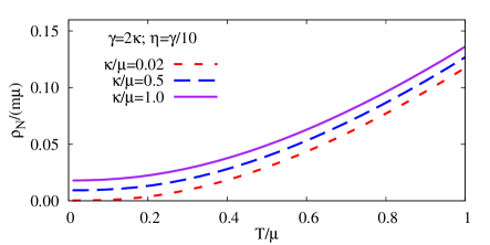
Figure 2: Normal density vs temperature for a variety of pump and decay rates and obeying the equilibrium fluctuation dissipation theorem. Relative pump and decay rates are scaled so all three curves correspond to the same condensate density, while the influence of pump and decay varies.

Having shown that superfluid density need not vanish in a dissipative condensate, but is reduced by finite lifetime, one may then ask how the superfluid and normal densities could be measured in such a system. As an illustration, the following suggests a method that uses the polariton polarization degree of freedom Shelykh et al. (2010) in order to apply ideas that have only recently been proposed for how one might measure of superfluid density in cold atom systems Cooper and Hadzibabic (2010); Dalibard et al. ; *Cooper2011. A number of alternative methods likely also exist, such as adaptations of proposals to create gauge fields in coupled photonic cavitiesHafezi et al. (2007); *Koch2010; *Umucalilar2011. To adapt the approach in Dalibard et al. ; *Cooper2011, one first considers the effective Hamiltonian $H_{B}$ due to an inhomogeneous real magnetic field, in the space of polariton polarization states. If the splitting of polarization states is always large, one may restrict to the adiabatic ground state $|\psi\rangle$. Because the polarization composition of this ground state varies in space, there can be a non-trivial synthetic gauge field in this subspace $q\boldsymbol{A}_{\text{synth}}=i\langle\psi|\nabla\psi\rangle$. Thus, a real magnetic field acting on polarization degrees of freedom can induce an artificial vector potential acting on the (neutral) polaritons. This artificial gauge field can mimic a rotating frame, thereby allowing one to distinguish the superfluid and normal response to rotation Leggett (2006).

In order to illustrate how this might work, one may consider the real magnetic field produced by an imbalanced anti-Helmholtz configuration, as illustrated in Fig. 3(a), so that the magnetic field in the microcavity has the form $\boldsymbol{B}=(\beta x,\beta y,B_{z})$ for small in-plane coordinates $x,y$ with constant $B_{z}$. Microcavity polaritons typically involve heavy-hole excitons, so that polariton polarizations $\pm 1$ imply electron and hole spins $(\mp 1/2,\pm 3/2)$. As such, while a B field perpendicular to the microcavity simply splits these polarization states, the in-plane field is more complicated, as it mixes the polariton states with non-radiative excitons with spins $(\pm 1/2,\pm 3/2)$. Furthermore, depending on the crystal symmetry and quantum well growth direction, the leading order coupling between $\pm 3/2$ hole states may either be linear or cubic in magnetic field Winkler (2003). In order to illustrate the basic idea, I will avoid these complications, and consider the simplest situation, where a linear coupling exists. Adiabatically eliminating the non-radiative excitons, the effective Hamiltonian for the polariton polarization is $H=\lambda[\ell^{2}\sigma_{z}+r^{2}(e^{2i\phi}\sigma_{-}+e^{-2i\phi}\sigma_{+})]$ where $re^{i\phi}=x+iy$ and the length $\ell$ encodes the ratio of in-plane and perpendicular fields. One may then find the ground state $|\psi\rangle$, ensuring this is smooth as $r\to 0$, and thus find $q\boldsymbol{A}=i\langle\psi|\nabla\psi\rangle=(\hat{\phi}/r)(1-l^{2}/\sqrt{r^{4}+l^{4}})$. This gauge field is equivalent to a rotating frame with $q\boldsymbol{A}_{\text{synth}}=m\boldsymbol{\omega}\times\boldsymbol{r}$ hence $\omega(r)=qA_{\phi}/mr$. This is shown in Fig. 3(b).

Detection of the response to this rotating frame could potentially be done by imaging the momentum and energy distribution of the polaritons Deng et al. (2010). If the condensate is concentrated around $r\simeq\ell$, one has the maximum velocity, corresponding to an energy shift for the normal component of $\Delta E_{\text{max}}=(1/2)mv_{\text{max}}^{2}=0.08/m\ell^{2}$. For $\ell\simeq 0.5\mu$m, and $m=10^{-4}m_{\text{electron}}$ this corresponds to $0.2$meV. Observing the differential shift of luminescence as one varies $\ell$ by varying $B_{z}$ could allow one to extract the superfluid fraction.

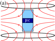
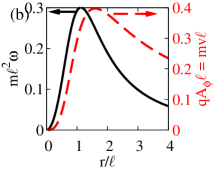
Figure 3: Panel (a), microcavity sample ($\mu c$) placed between (imbalanced) anti-Helmholtz coils to induce a field $\boldsymbol{B}_{\text{real}}$. Panel (b), velocity and angular velocity vs radius for $\boldsymbol{A}_{\text{synth}}$ as discussed in the text.

I now turn to discuss in more detail how the superfluid density can be calculated in the Schwinger-Keldysh approach, and to explain the origin of the vertex corrections in Fig. 1 and the form of the normal density in Eq. (3). Following the path integral approach to the Schwinger-Keldysh formalism Altland and Simons (2010); *kamenev05, the response function can be written in terms of a generating functional as:

$$\chi_{ij}(q)=\frac{-i}{2}\frac{d^{2}\mathcal{Z}[f,\theta]}{df_{i}(q)d\theta_{j}(-q)},\ \ \mathcal{Z}=\!\!\int\!\mathcal{D}(\bar{\psi},\psi)e^{i(S+\delta S)}.$$ (4)

Here, $S$ is the Keldysh action Altland and Simons (2010); *kamenev05 due to the Hamiltonian in Eq. (2) and the pump and decay terms $S=\sum\bar{\psi}_{\boldsymbol{k}}\mathcal{D}_{0}^{-1}{\psi}_{\boldsymbol{k}^{\prime}}-\iint dtd^{2}r\frac{U}{2}[\bar{\psi}_{q}\bar{\psi}_{cl}(\psi_{cl}^{2}+\psi_{q}^{2})+\text{H.c.}]$ where the fields $\psi$ are written in the Keldysh space for classical/quantum fields Altland and Simons (2010); *kamenev05, and the retarded, advanced and Keldysh components of the inverse Green’s function $\mathcal{D}^{-1}_{0}$ are as discussed above. The source term $\delta S=\sum\bar{\psi}_{\boldsymbol{k}+\boldsymbol{q}}[\tau_{1}f_{i}(q)+(\tau_{3}+i\tau_{2})\theta_{i}(q)]\gamma_{i}(2\boldsymbol{k}+\boldsymbol{q}){\psi}_{\boldsymbol{k}}$, where Pauli matrices $\tau_{i}$ are in the Keldysh space. The presence of two separate fields is necessary due to need to calculate a normal ordered current (derivative with respect to $\theta$) linearly dependent on a classical force (field $f$).

In the non-condensed state, one may immediately determine $\mathcal{Z}$ at leading order by neglecting interactions, and performing the (Gaussian) integration over fields $(\bar{\psi},\psi)_{cl,q}$. This yields $m\chi_{ij}=\rho_{n}\delta_{ij}$, with $\rho_{n}$ given by Eq. (3), where the Nambu structure in the normal state is trivial. When condensed, vertex corrections become important. These vertex corrections can be found by use of an “honest saddle point” of the partition function, i.e. determine the saddle point in the presence of the source terms $f,\theta$, and then integrate out fluctuations about this new saddle point. One thus finds a form $\mathcal{Z}\propto\exp\{iS_{0}[f,\theta]-\frac{1}{2}\text{Tr}\ln(1+\mathcal{D}A[f,\theta])\}$ where $S_{0}$ is the saddle point action, $\mathcal{D}$ are the Green’s functions (for $f=\theta=0$) and $A$ is the self energy due to the fields $f,\theta$. Both $S_{0}$ and $A$ involve terms arising from the shift of the saddle point field $\psi$ in the presence of the source terms $f,\theta$, and thus both $S_{0}$ and $A$ have higher order contributions of $f,\theta$. One may then expand these terms to quadratic order in $f,\theta$ and evaluate $\chi_{ij}$ via Eq. (4).

Taking derivatives with respect to $f,\theta$ (indicated by primes and subscripts), one finds $\chi_{ij}=\frac{1}{2}S^{\prime\prime}_{0,f_{i},\theta_{j}}+\frac{i}{4}\text{Tr}(\mathcal{D}A^{\prime\prime}_{f_{i}\theta_{j}})-\frac{i}{4}\text{Tr}(\mathcal{D}A^{\prime}_{f_{i}}\mathcal{D}A^{\prime}_{\theta_{j}})$. Comparing the three terms in this expression to the diagrams in Fig. 1 the first diagram arises from the first term, the second two diagrams arise from the second term, and the last three diagrams from the third term. After explicitly evaluating the shifts to the saddle point, and the self energy $A$, one finds the explicit form:

$$m\chi_{ij}(q)=\frac{q_{i}q_{j}}{q^{2}}\left\{\frac{\Lambda}{U}+m\!\!\int\!\frac{d\epsilon_{k}}{2\pi}\left[1-\frac{i}{4}\int\frac{d\omega}{2\pi}\left(\text{Tr}\left[\left(2\sigma_{0}+\sigma_{1}\right)D^{K}_{k}\right]-\frac{2\Lambda}{\epsilon_{q}}\text{Tr}(D^{K}_{k}\sigma_{1})\right)\right]\right\}\\ -m\!\!\int\!\frac{d\epsilon_{k}}{2\pi}\left[\frac{q_{i}q_{j}}{q^{2}}2\frac{\Lambda^{2}}{\epsilon_{q}}N_{22}-i\frac{q_{i}(q_{j}+2k_{j})}{q^{2}}\Lambda N_{23}+i\frac{(q_{i}+2k_{i})q_{j}}{q^{2}}\Lambda N_{32}+\frac{(q_{i}+2k_{i})(q_{j}+2k_{j})}{4m}N_{33}\right]$$ (5)

where $N_{ab}=\int\frac{id\omega}{8\pi}\text{Tr}(D^{R}_{k+q}\sigma_{a}D^{K}_{k}\sigma_{b}+D^{K}_{k+q}\sigma_{a}D^{A}_{k}\sigma_{b})$ in terms of Pauli matrices $\sigma_{i}$ in the Nambu space and $\Lambda=U|\psi_{0}|^{2}$. The terms in Eq. (5) are arranged in the same order as the corresponding diagrams in Fig. 1.

A number of technical issues regarding regularization are worth noting. Firstly, as is known elsewhere (see e.g. Wilson and Galitski (2011) and refs. therein), there can be cases where it is necessary to return to the discrete time coherent state path integral in order to correctly incorporate causality in performing integrals. The current problem is such a case, and the term arising from this is the $1$ on the first line of Eq. (5). Secondly, in order to give an ultraviolet finite expression, it is necessary to perform the standard T-matrix regularization of the contact interaction: $U^{-1}\to U_{\text{eff}}^{-1}-m\int\frac{d\epsilon_{k}}{2\pi}[2(\epsilon+\mu)]^{-1}$. Thirdly, the apparently singular terms involving $q_{i}q_{j}/q^{2}\epsilon_{q}$ in fact cancel, leaving only finite contributions as $q\to 0$. One may verify that Eq. (5) recovers the expected equilibrium result in the absence of pumping and decay.

One may note that the expression in Eq. (5) does not explicitly involve details of the pumping. This is because the only nonlinearity included being the interaction term $U$. This means that Eq. (5) survives for general models of pumping and decay, and so is more generic than the particular model of pumping used to derive it.

In conclusion, the superfluid density of a non-equilibrium open dissipative condensate need not vanish, despite the non-existence of a Landau critical velocity. This is because the poles of the response function, which give the spectrum, do not uniquely determine the form of the response function at zero frequency, which is the quantity that defines the superfluid density. Such a superfluid density could potentially be measured in a polariton system by using real magnetic fields to engineer an effective rotating frame. The current-current response function can be explicitly calculated using the “honest saddle point” approach. Such an approach would also allow calculation of dynamical response functions, allowing a more nuanced understanding of the distinctions between static and dynamic superfluid phenomena in open dissipative condensates.