Stochastic theory of protein synthesis and polysome:
ribosome profile on a single mRNA transcript
Abstract
The process of polymerizing a protein by a ribosome, using a messenger RNA
(mRNA) as the corresponding template, is called translation. Ribosome
may be regarded as a molecular motor for which the mRNA template serves
also as the track. Often several ribosomes may translate the same (mRNA)
simultaneously. The ribosomes bound simultaneously to a single mRNA
transcript are the members of a polyribosome (or, simply, polysome).
Experimentally measured polysome profile gives the distribution of
polysome sizes. Recently a breakthrough in determining the instantaneous
positions of the ribosomes on a given mRNA track has been achieved and
the technique is called ribosome profiling ingolia10 ; guo10 .
Motivated by the success of these techniques, we have studied the
spatio-temporal organization of ribosomes by extending a theoretical model
that we have reported elsewhere sharma11 .
This extended version of our model incorporates not only (i) mechano-chemical
cycle of individual ribomes, and (ii) their steric interactions, but also
(iii) the effects of (a) kinetic proofreading, (b) translational infidelity,
(c) ribosome recycling, and (d) sequence inhomogeneities. The theoretical
framework developed here will serve in guiding further experiments and in
analyzing the data to gain deep insight into various kinetic processes
involved in translation.
Key words: ribosome traffic, master equation, extremum current hypothesis, distance-headway, TASEP.
pacs:
87.16.Ac 89.20.-aI Introduction
Ribosome spirin00 ; spirin02 ; frank06 is a macromolecular complex and operates as one of the essential intracellular machines frank11 that participate in gene expression in all living cells alberts ; lodish . More specifically, it polymerizes a protein that is a linear hetero-polymer consisting of amino-acid monomers each of which is linked to the next one by a peptide bond. Therefore, growing protein is also called a polypeptide. For the synthesis of a protein, a messenger RNA (mRNA) serves as the template; the sequence of the amino acid species in the protein is determined by that of the codons (triplets of nucleotides) on the corresponding mRNA template. This process is called translation. Translation by every ribosome goes through three main stages: (i) initiation, (ii) elongation, and (iii) termination. The start and stop codons mark the positions on the template mRNA where initiation and termination of translation take place.
During the elongation stage, at every codon, the amino acid monomer required for elongating the protein is supplied by an incoming tRNA molecule; the correct amino acid monomer is carried by those tRNA whose anti-codon is complementary to the codon. The machinery of translation deploys a quality control mechanism which screens the incoming tRNA through a multi-step selection process. However, in spite of this stringent selection process, occasionally an incorrect amino acid may escape rejection by the quality control system; a translational error results if the growing protein incorporates an incorrect amino acid monomer thereby lowering the fidelity of translation. In any case, after the termination, a ribosome is partly disassembled. These parts can reach near the start codon by diffusion in the surrounding aqueous medium. A ribosome can be assembled more quickly from these parts than from basic constituents. Moreover, in case the start and the stop codons are close to each other because of the loop formation by the mRNA, diffusive transfer of the parts of the ribosome from the stop codon to the start codon can be quite rapid leading to a faster recycling of the ribosomes hirokawa06 . Rarely elongation process is aborted because of the premature detachment of the ribosome from the mRNA track. Furthermore, often several ribosomes translate the same mRNA transcript simultaneously, each polymerizing a distinct copy of the same protein. Because of the superficial similarities with vehicular traffic on a given stretch of a highway css00 ; scn10 ; polrev05 , the simultaneous collective translation of a mRNA by several ribosomes is sometimes referred to as ribosome traffic. The ribosomes bound simultaneously to a single mRNA transcript are the members of a polyribosome (or, simply, polysome) warner62 ; warner63 ; rich04 ; noll08 . Because of the mutual hindrance of the ribosomes, the overall rate of protein synthesis is expected to attain a maximum at an optimum mean separation between the ribosomes. Finally, the ongoing production and decay of mRNA transcripts and various feedback loops in gene expression also control the rate of protein synthesis.
It would be desirable to capture all the processes mentioned above within a single theoretical model of translation. However, it is extremely unlikely that such a model can be analyzed analytically. Therefore, the aim of this paper is more modest. Here we extend our earlier model sharma10 ; sharma11 . capturing (i) the mechano-chemical cycle of individual ribomes, and (ii) their steric interactions, as well as (iii) the effects of (a) quality-control mechanisms, (b) translational error, (c) ribosome recycling, and (d) sequence inhomogeity of the mRNA.
The overall rate of synthesis of proteins is a key quantity in any model of translation. However, the main focus of our theoretical study here are the size of the polysome and the spatial distribution of ribosomes on a mRNA. We identify the different parameter regimes of our theoretical model and characterize these in terms of the average density of the polysome and the overall average rate of synthesis of proteins from a single mRNA transcript. Moreover, going beyond the scope of all the previous theoretical works on this topic, we predict the nature of the fluctuations in the spatial organizations of the ribosomes which throws light on the fluctuations in the size of ribosome clusters on a given mRNA transcript.
In this paper we also suggest a new experiment for testing our theoretical predictions on the statistical properties of polysomes. Traditional technique of polysome profiling arava03 ; mikamo05 provide the number of ribosomes bound to a mRNA, but not their individual position at the instant when translation was stopped by the experimental protocol. An improved version of this technique, called ribosome density mapping arava05 , provides more detailed information on the numbers of ribosomes associated with specified segments of a particular mRNA by carrying out site-specific cleavage of the mRNA transcript. The results obtained using these techniques are often adequate for getting a qualitative indicator of the translational activity. However, the ribosomes are not expected to be uniformly distributed on a mRNA because of the stochasticities in the steps of the mechano-chemical cycles of these cyclic machines. These stochasticities arise from (i) intrinsic fluctuations in biochemical processes at low copy numbers of the molecules, and (ii) extrinsic fluctuations arising from the sequence inhomogeneity of the mRNA. The most detailed picture of the translational activity has been obtained by a recently developed technique, called ribosome profiling ingolia10 ; guo10 . For testing some of our theoretical predictions, the older technique of polysome profiling is adequate whereas for testing the other new results ribosome profiling would be necessary.
This paper is organized as follows: we introduce our model and write down the master equations for the stochastic kinetics of this model in section II. In section III we solve the master equations in the steady state under periodic boundary conditions to calculate the overall rate of protein synthesis. The results demonstrate the effects of steric hindrance caused by congestion ribosome traffic. The spatio-temporal organization of the ribosomes in different parameter regimes correspond to the different non-equilibrium phases on the “phase diagrams” which we plot in section IV. The instantaneous spatial distribution of the ribosomes on a single mRNA is also characterized in terms of some quantitative measures which we introduce in section V where we also explore the effects of sequence inhomogeneities of mRNA. Finally, in section VI, the main results are summarized and important conclusions are drawn.
II Model
The kinetic models of translation can be divided into three categories. Translation is just a single step in the broader context of gene expression. However, in most of the kinetic models of gene expression zhdanov11 , the details of the mechano-chemistry of individual ribosomes as well as their mutual steric interactions are ignored. The rates of synthesis and degradation of proteins are captured usually in these models by two rate constants without any mechanistic details of these two processes. We are not concerned with a global picture of gene expression in this paper and, therefore, such kinetic models will not be discussed further here.
There are models of translation which are intended to describe various key aspects of the stochastic mechano-chemical kinetics of only a single ribosome. In contrast, another class of models of translation is motivated by the polysome formation. Most of these models capture the effects of entire mechano-chemical cycle by a single parameter. These models focus mainly on the effects of mutual steric interactions of the ribosomes on the overall rate of protein synthesis. In this section we develop a model by capturing both these aspects of translation, namely, details of single-ribosome mechano-chemistry and the effects of steric interactions among the ribosomes on the same mRNA transcript. However, for the convenience of comparison of our work with earlier works, we summarize the main features of the TASEP-type models in the next subsection.
II.1 TASEP-type models
Totally asymmetric simple exclusion process (TASEP) derrida ; schuetz is one of the simplest models of interacting self-propelled particles; it is used extensively for understanding the generic features of non-equilibrium steady-states of interacting systems. TASEP and its various extensions exhibit interesting dynamical phase transitions mukamel00 . For many years, various biologically motivated extensions of TASEP macdonald68 ; macdonald69 ; lakatos03 ; shaw03 ; shaw04a ; shaw04b ; chou03 ; chou04 ; zia11 ; zouridis08 ; romero10 have been used to model ribosome traffic. In the TASEP-based models of ribosome traffic (see ref.zia11 for a recent review) each lattice site represents a single codon. Since a ribosome is much larger than a single codon, each ribosome is represented by a hard rod that covers () sites simultaneously. But, the allowed step size of a rod is one lattice site (i.e., one codon). This extended version of TASEP for hard rods will be referred to as -TASEP. As long as a site remains covered by a ribosome, it is inaccessible to the other rods. The entry of a rod from one end (at a rate ) and its eventual exit from the other end (at a rate ) model the initiation and termination stages of translation by a ribosome.
The steps of the mechano-chemical cycle of individual ribosomes during the elongation stage were not captured explicitly in the simple TASEP-type models; instead, one single “hopping” parameter was used to describes the rate of translation of one codon. Moreover, these TASEP-type models neither incorporate any mechanism for selecting specifically the correct amino acid monomer, nor do these allow for the possibility of translational error. Therefore, such TASEP-type models are too simple to account for the effects of various mechano-chemical processes on the statistical properties of polysomes.
II.2 Our model: unification of single-ribosome mechano-chemistry and TASEP
In recent years, progressively more realistic models of translation have been developed ciandrini ; basu07 ; gccr09 ; sharma10 ; sharma11 and several analytical results have been derived. Using the most recent version of this model sharma11 , some statistical properties of single ribosome have been derived analytically sharma11 . Here we extend this model even further to capture some features of translation which were not included in its earlier version. Using this extended version of our model of translation, we make experimentally testable predictions on the dependence of the statistical properties of the polysomes on the various mechano-chemical processes involved in translation.
Each ribosome consists of two subunits which are designated as “large” subunit and “small” subunit, respectively. The translation of the genetic message encoded in the codon is carried out by the small subunit while the elongation of the polypeptide, by the formation of a peptide bond between it and the incoming amino acid, takes place in the large subunit. The function of the two subunits is coordinated by the tRNA molecules. There are three binding sites for a tRNA on each ribosome; these sites are designated as E,P and A. An incoming tRNA binds with an A site. The amino acid carried by a tRNA is linked to the growing polypeptide by a peptide bond while the tRNA is bound to the P site. Finally, the denuded tRNA exits from the ribosome from the E site. During the elongation stage, in each complete mechano-chemical cycle, the ribosome steps forward on the template mRNA by one codon while, simultaneously, the polypeptide gets elongated by one amino acid. These processes are captured explicitly in the our kinetic model.
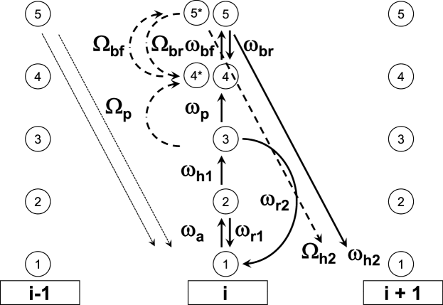
The distinct mechano-chemical states in our model and the allowed transitions among these states are shown schematically in fig.1. At the beginning of each cycle, the system is in state 1 where the sites E and A are empty while the site P is occupied by a tRNA that has just contributed its amino acid to the growing polypeptide. A tRNA charged with an amino acid is called a aminoacyl tRNA (aa-tRNA). At this stage, an aminoacyl tRNA, bound to an elongation factor Tu (EF-Tu) and a molecule of Guanosine triphosphate (GTP) enters and binds with the A site on the Ribosome at the site A. This process takes place with rate which causes transition of the system to the chemical state 2. Thereafter non-cognate tRNAs are rejected, and the system reverts back to state 1, with rate , through a quality control mechanisms based on the free energy of codon-anticodon matching.
However, the free-energy difference between the cognate and near-cognate tRNAs is too small to distinguish between them. Therefore, usually, near-cognate tRNAs are not rejected at this stage. A second stage of quality control, called kinetic proofreading hopfield ; ninio , is then activated. GTP, which is bound to the aa-tRNA, is hydrolyzed to GDP by EF-Tu and this process is described by the transition from the state to the state . At this stage, barring a few exceptional cycles, the near cognate tRNAs are rejected from chemical state 3 which drives the system back to the chemical state 1; this happens with rate constant .
Although most often the noncongnate and near cognate tRNAs are rejected by the two-stage selection process, still occasionally the quality control system fails to reject an incorrect (non-cognate or near-cognate) tRNA. Consequently, there is a small, but non-vanishing probability, of a translational error when the growing polypeptide elongates by the formation of a peptide bond with an incorrect amino acid. In our model, the incorporation of incorrect amino acid leads to a branched pathway: in contrast to the transition along the correct pathway, the wrong pathway proceeds by the transition . Arrival of another elongation factor called EF-G, alongwith a molecule of GTP also takes place at this stage. The transition (or, ) is reversible and essentially a Brownian rotation of the two subunits relative to each other. This spontaneous Brownian rotation drives the two tRNA molecules back-and-forth between the classical P/P, A/A state and the hybrid E/P, P/A state agir09 . The rate constants for the forward and backward Brownian rotations are denoted by and , respectively, along the correct pathway whereas the same transitions along the wrong pathway take place with the rates and , respectively. Finally, hydrolysis of GTP by EF-G drives the process of translocation at the end of which the two tRNA molecules are positioned at the E and P sites while the ribosome finds itself poised to translate the next codon; the denuded tRNA molecule makes an exit from the E site. The transition and take place with the rates and , respectively. The completion of the full cycle elongates the protein by one amino acid (by correct amino acid along one pathway and by an incorrect amino acid along another branch) and translocates the ribosome by one codon on the template mRNA (For further details, see ref.agir09 ).
Since our model allows the possibility of translational error, we define sharma10 the fidelity of translation by the fraction of the incorporated amino acids which are correct, i.e.,
| (1) |
In our model, the mRNA track is represented by a one-dimensional lattice where each of the total sites corresponds to a single codon. The length of a ribosome is denoted by in the units of the length of a single codon. A ribosome can move forward by only one site (i.e., one codon) at a time. We use the convention that the leftmost site covered by a ribosome is the one that is being translated by it; the leftmost site covered by a ribosome is also used in our formulation to denote the position of a ribosome. Thus, throughout this paper, we follow the convention that, at any instant of time, a ribosome “covers” sites but “occupies” only the leftmost of these sites.
According to our notation, the status of coverage of a site is denoted by and ; represents an unoccupied lattice site whereas represents a covered site. Since many ribosomes move simultaneously on the same track they also interact with each other. The simplest form of interaction would be mutual exclusion: if the th site is “occupied” by one ribosome, then all the sites from to are “covered” by it and, therefore, none of the these sites are accessible to any other ribosome at that instant of time. Moreover, a ribosome occupying the position can move forward if, and only if, the site is not simultaneously occupied by another ribosome. In our notation, the symbol represents the conditional probability that, given an uncovered site, there will be successive adjacent sites to its left all of which are covered simultaneously by a single ribosome. Similarly, is the conditional probability of finding a empty site , given that the successive sites on its left are covered by a ribosome.
Using the same notation, we now define as the conditional probability that the site is not occupied by another ribosome, given that the site is occupied by a ribosome, Similarly, given that the site is occupied by a ribosome, the probability that the site is not occupied by another ribosome is given by the conditional probability . It is straightforward to show that basu07 ; gccr09
| (2) |
Where is the number density of the Ribosome on the track. Following the same prescription that one of us (DC), and his collaborators, used in earlier simpler models of ribosome traffic basu07 ; gccr09 , we multiply the rate constants and by Q because a ribosome “feels” the mutual exclusion only when it tends to move forward to the next codon.
By the symbol we denote the probability of finding the ribosome in the th chemical state while it occupies the site at time . The master equations for the probabilities are
| (3) |
| (4) |
| (5) |
| (6) |
| (7) |
| (8) |
| (9) |
Equations (3)-(7) correspond to the equations (52)-(56) of ref.gccr09 . However, there are some additional terms in (3)-(7) because of (i) the kinetic proofreading, (ii) translational because of wrong amino acid selection, and (iii) reversible nature of the transition between the states and . Moreover, the precise interpretations of the respective states were slightly different in ref.gccr09 (see ref.gccr09 for the detailed interpretations of the states and transitions between the states).
Note that the normalization condition for the probabilities is
| (10) |
Molecular mechanisms that lead to mistranslation have been under intense investigation for decades (see reynolds10 for a recent review). However, to our knowledge, none of the earlier models, including that developed in ref.gccr09 , provides a mathematical framework to treat the mechanisms of mistranslation analytically.
III Rate of protein synthesis: effects of hindrance in ribosome traffic
We solve the equations (3)-(9) in the steady state under normalization condition (10) and imposing periodic boundary conditions (PBC). Using the steady-state solutions for we get the following expression for the steady-state flux
| (11) |
where
| (12) | |||||
Separating out the -dependent and -independent parts, can be re-expressed as
| (13) |
where
| (14) | |||||
and
| (15) |
Note that when simultaneously , , , the expressions for and reduce to and , respectively.
So the is given by
| (16) |
Since no premature detachment of ribosomes are allowed in our model, the flux of the ribosomes is also the total rate of protein synthesis. In the special case the expression (16) reduces to the corresponding expression for flux derived in ref.gccr09 . The expression (16) for exhibits a single maximum which occurs at the number density
| (17) |
The equations (16) and (17) reduce, respectively, to the equations (58) and (63) of ref.gccr09 .
IV Nature of polysomes: non-equilibrium phase diagram of ribosome traffic
In this section we impose open boundary conditions (OBC) which is more realistic for modeling translation. The entry of the ribosomes at one open end captures the initiation of translation while the exit of the ribosomes from the other open end mimics termination of translation.
IV.1 Phase diagram
In a multi-dimensional abstract space spanned by some of the crucial model parameters, we identify the distinct regions characterized by their distinctive properties which we describe below. The resulting diagram is referred to as a “phase” diagram although the “phases” are not in thermodynamic equilibrium; these phases are non-equilibrium steady states of the system. The theoretical prediction we make in this section can be tested by using the technique of polysome profile arava03 ; mikamo05 .
Our calculations here are based on the extremum current hypothesis (ECH) krug91 ; popkov2 ; hager1 ; hager2 which relates the flux , under OBC, to the flux of the same system, under PBC. We apply the ECH to our model in the same way in which it was used earlier for the simpler versions of our model basu07 ; gccr09 . We assume that the entrance and exit points of the track (i.e., the start and stop codons) are connected to two infinite particle reservoirs where the respective number densities are and , respectively. According to ECH, for systems with a single maximum in the function,
| (18) |
These relations can be utilized to draw the surfaces separating the dynamical phases on the phase diagram. The first step in this approach has already been completed by calculating the expression (17) for . Next, we derive the expressions for and which would give rise to the same rates of initiation and termination as indicated by and , respectively.
Suppose is the probability that, given an empty site, a ribosome will hop onto it from left in the next time interval . It is straightforward to see that
| (19) |
where and are given by the expressions
| (20) |
and
| (21) |
respectively, and as discussed in ref.gccr09 ,
| (22) |
Note that the solutions (20) and (21) have been obtained using the normalization condition
| (23) |
for the reservoir.
Now is the solution of the equation . Hence,
| (24) |
with
| (25) |
relating the probability with the rate constant where is given by (15). Similarly,
| (26) |
where
| (27) |
The unknown density is the solution of the equation ; hence,
| (28) |
Note that the equations (24) and (28) reduce, respectively, to the equations (67) and (70) of ref.gccr09 in the appropriate limit.
IV.1.1 Surface separating LD and MC phases
From MCH it follows that the surface separating the LD and MC phases on the phase diagram of the system is obtained from the equation
| (29) |
by expressing and in terms of the rate constants for the elementary steps of the model kinetics. Hence, the equation for this surface in the phase diagram of the model is found to be
| (30) |
IV.1.2 Surface separating HD and MC phases
Similarly, using the condition
| (31) |
the equation for the surface separating the HD and MC phases in the phase diagram of the system is given by
| (32) |
IV.1.3 Surface of coexistence of HD and LD phases
| (33) |
which gives
| (34) |
Equivalently
| (35) |
Note the equations (30), (32), (34) and (35) reduce to the expressions (72), (74), (76) and (77), respectively, of ref.gccr09 in the appropriate limit.
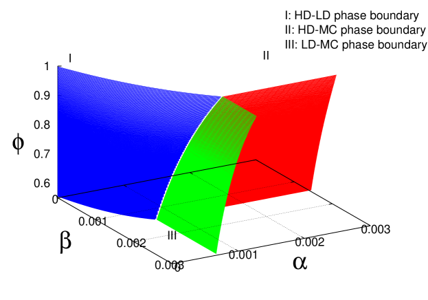
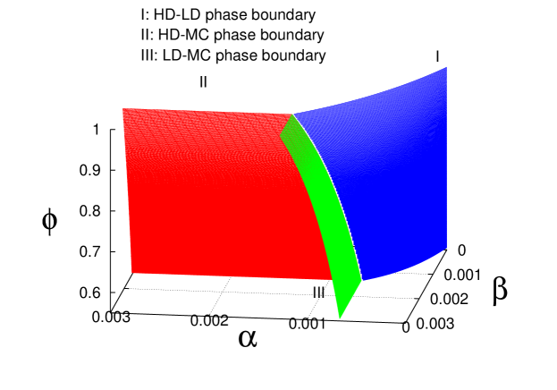
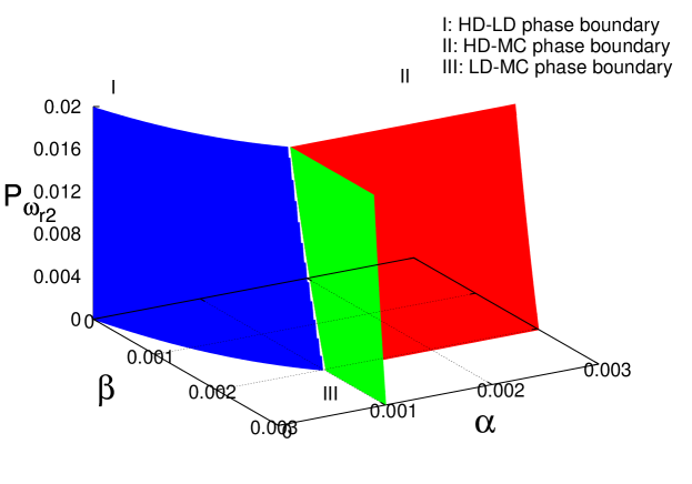
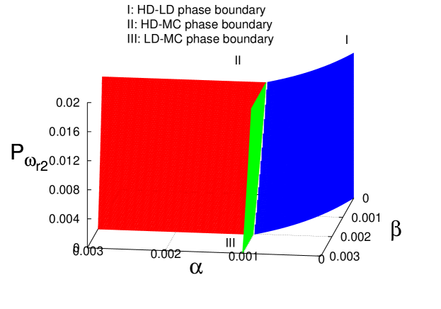
Figs.2 and 3 show the 3-dimensional phase diagrams plotted in the space from two different perspectives, while figs.4 and 5 show the 3-dimensional phase diagrams plotted in the space also from two different perspectives. Since none of the earlier models of ribosome traffic capture translational fidelity and kinetic proofreading explicitly, these phase diagrams have not been reported ever before.
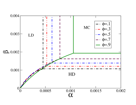
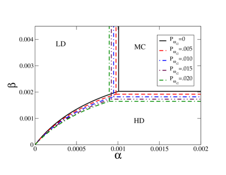
In order to compare the implications of these phase diagrams with that of the TASEP, we also project several two-dimensional cross sections of these phase diagrams onto the -plane (see figs.6 and 7). On the 2D projections, transition from the LD phase to the MC phase takes place at whereas the transition from the HD phase to the MC phase takes place at .
As is evident from these 2D phase diagrams, the curvature of the lines of coexistence of HD and LD phases seems to be the generic feature of all such models gccr09 ; antal00 . The straight line on which the LD and HD phases of TASEP coexist is a manifestiation of the “particle-hole” symmetry in TASEP, a special property that is not shared by our model of ribosome traffic.
Increasing shifts and to higher values. Increase of can be viewed as a result of increasing which, in turn, increases the effective rate of hopping of a ribosome from one codon to the next. It is well known kolo98 that higher values of effective hopping rate shifts and to higher values. Similarly, increasing decreases the effective hopping rate thereby shifting and to smaller values.
IV.2 Effects of recycling on the phase diagram
Recycling of ribosomes can be captured by our model by replacing the constant initiation rate by an effective initiation rate . Since the availability of ribosomes for initiation is proportional to the flux of ribosomes exiting from the stop codon, we postulate that
| (36) |
where the coefficient depends on the relative separation between the two ends of the transcript as well as on the diffusion constant of the ribosome subunits in the solution.chou03 . Note that the prescription (36) for recycling is similar in spirit, but not identical quantitatively, to the prescription used by Gilchrist and Wagner gilchrist06 because the latter model does not capture steric exclusion among the ribosomes.
On simple physical grounds, the effect of (36) on the phase diagram is expected to be non-trivial. Suppose, is varied keeping fixed. At a very small value of (), the flux would be determined by . Starting from a very small value, increasing initially increases which, in turn, increases the effective initiation rate . However, beyond a certain value of , is no longer rate limiting and the flux becomes independent of .
Exploiting the relation between our model and -TASEP, we plot the phase diagram for the extended model that captures recycling of ribosomes through . We use the results reported in refs.shaw03 ; zia11 for - and get
| (37) |
| (38) |
which gives
| (39) |
So at LD and HD interface
| (40) |
at LD and MC boundary
| (41) |
and at HD and MC boundary
| (42) |
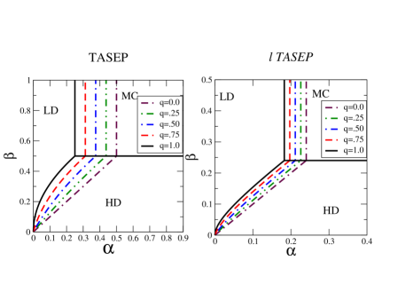
The resulting 2-d phase diagram in the plane is plotted in fig.8. Increase of the recycling factor shifts to a smaller value while remains unchanged. This trend of variation is consistent with the fact that recycling affects only the initiation rate without influencing the rate of termination. This is consistent with the trends of variation of the coverage density and flux of ribosomes that we observed in our computer simulations which we descibe below.
IV.2.1 Variations of flux and coverage density with the extent of recycling
In order to demonstrate the effects of recycling in a form that would be closer to one’s physical intuition, we now show the variation of the average flux and the average coverage density of the ribosomes with the parameter which is a measure of the extent of recycling. For this purpose, we carried out computer simulations of our model for several different values of . All the data reported here were obtained for and . Since the linear size of a ribosome is measured here in the units of codons, is a realistic choice because in recent experiments ingolia10 ; guo10 it has been observed that each ribosome covers about 30 nucleotides on the mRNA track. Typical values of some of the rate constants have been reported in the literature thompson80 ; harrington93 . For those rate constants whose numerical values are not available in the literature, we have assumed some reasonable values based on physical intuition. However, our conclusions are not sensitive to the precise numerical values of the rate constants.
The rate constants which we used for the simulations are
=25, =25,=25,=25,=25,=25,10,10,=5,=5,=5,=5
All the rate constants were converted to dimensionless transition
probabilities using the formula
where time step s is used for all the simulation runs.
At first sight, it may appear that there is some ambiguity in the defnition of : what value of should be used in (36)? In order to avoid ambiguity, we average the spatially-averaged flux further over the time period elapsed since the last entry of a ribosome (i.e., the initiation of translation by the ribosome closest to the start codon). This “doubly-averaged” value of flux is used in (36) to compute .
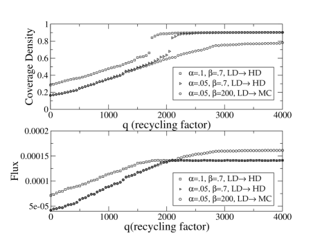
In fig(9) we plot the flux and the coverage density of the ribosomes as functions of . Starting from a vanishingly small value, as is increased, both the flux and coverage density increase. However, beyond a limiting value, both become practically independent of ; this trend of variation is caused by a transition from the LD phase to either the HD phase or to the MC phase, depending on the values of the set of other parameters.
‘
IV.3 Experimental tests of the phase diagram with polysome profile
The three different phases are characterized by three different densities; the expressions for these densities have been derived above. Therefore, our theoretical predictions can be tested by measuring the average densities. For this purpose, polysome profiling arava03 ; mikamo05 would be adequate. However, all the analytical calculations for the phase diagram have been carried out for sequence-homogeneous mRNA strands. Therefore, a poly-U strand of mRNA, with appropriate start and stop codons sharma11 , should be used in the experiment.
‘
V Instantaneous spatial distribution of ribosomes: ribosome profile
In all the sections above we have calculated quantitative characteristics which do not require information on the spatial distributions of the ribosomes on the mRNA transcript. In this section we explore some other quantitative features of ribosome traffic which deal with the spatial distributions of the ribosomes. Our theoretical predictions on the spatial distributions of the ribosomes can be tested with the ribosome profiling technique guo10 ; ingolia10 .
‘
V.1 Distance-headway distribution
The distance-headway (DH) is defined as the spatial separation between two successive ribosomes on the same mRNA transcript. At any given instant of time, the magnitude of the DH fluctuates from one pair of ribosomes to another, the instantaneous spatial distribution of the ribosmes is characterized by the corresponding distribution of the DHs. The DH distribution is used extensively for quantitative characterization of macroscopic vehicular traffic css00 ; scn10 . In this subsection we calculate the DH distribution for our kinetic model of ribosome traffic. Since ribosome profiling ingolia10 ; guo10 provides the exact positions of the ribosomes at the instant when translation was stopped, DH distribution can be extracted by repeatiting this profiling sufficiently large number of times.
Our system may be viewed as one that consists of identical rods, each of length , distributed over a lattice of sites. First, assuming a ring-like mRNA track we get the DH distribution for the corresponding number density which, because of the PBC, does not fluctuate. In this case, the expression for the DH distribution is given by shaw03
| (43) |
where is the density of holes and . Hence,
| (44) |
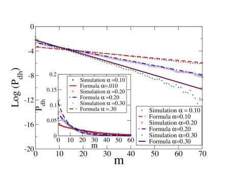
The number density of the ribosomes for the real system under OBC is a fluctuating quantity. But, the mean density deep inside the bulk (around the central region of the lattice) can be extracted numerically from computer simulations. Substituting the numerically estimated density of the ribosomes under OBC into the expression (44) we get the DH distribution under OBC. This distribution is plotted in fig.10. The straight lines on the semi-log plot reflects the geometric nature of the distribution (discrete analog of the exponential distribution). In order to test the validity of the approximate scheme used above to derive the DH distribution by a combination of analytical and numerical arguments, we have also computed the DH distribution directly by computer simulation; the simulation data are also plotted in fig.10. The theoretically derived lines are in reasonaly good agreemwnt with the DH distribution obtained by computer simulation.
‘
V.2 Influence of slow codons on the density profile and flux
It is well known that translation of some codons take place at a very slow rate; these are often referred to as “hungry” codon. However, we’ll use the term “slow” to refer to the all those codons which get translated at a much slower rate than other codons. In this subsection we explore the effects of bottlenecks created by such slow codons against the forward movements of ribosomes. In particular, we investigate the effects of slow codons on the average density profile and flux of ribosomes in ribosome traffic.
In the model that we simulated for this purpose, a transcript consists of only two different types of codons. In the computer simulations of our model we assign ten times smaller numerical value to for a slow codon compared to that of a normal codon. Simultaneously, the numerical value of assigned to a slow codon is ten times larger than that of a normal codon. Since in this particular study we are interested mainly in the effects of bottlenecks, we ignore the possibility of misincorporation by erasing the branched pathway putting .
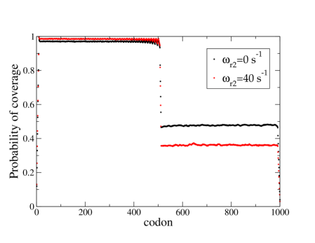
In the first set of simulations, we put four slow codons at the center of the stretch of mRNA between the start and the stop codon. Such a single extended bottleneck leads to a “phase-segregated” profile where on one side of the bottleneck the average density is much higher than that on the other side (see fig11). Profiles are plotted for different values of . Higher value of reduce the effective hopping rate for both normal as well as rare codons. But, the effective hopping rate for slow codon decrease more because of higher value of . Thus, the higher is the value of , the larger is the difference between the effective rates of hopping from normal and slow codons. This, in turn, leads to the larger jump discontinuity of the density across the bottleneck at a larger value of .
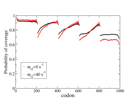
In the second set of simulations, the slow codons were not clustered together. Instead, four equispaced slow codons were placed at the sites , and on a lattice of total length .The average density profiles for this case are plotted in fig.12 for two different values of . Both the profiles exhibit discontinuous jumps in the coverage density; the position of each minimum in the coverage density coincides with the location of a slow codon. Moreover, periodic oscillations are also observed in the vicinity of the the rare codon where periodicity is . Similar results were obtained earlier in TASEP-type models of ribosome traffic zia11 ; however, unlike our data, shown in fig.12, the effects of kinetic proofreading and futile cycles could not be addressed by the model of ref.zia11 .
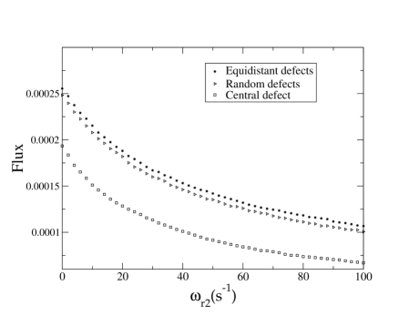
In order to emphasize the effect of clustering of slow codons on the overall rate of protein synthesis we plot flux as a function of in fig13 for the two different conditions discussed above. The upper curve corresponds to the setup where four slow codons are placed equidistant on lattice. The lower curve corresponds to the setup where all the four slow codons are placed clustered together at the center of the system. The data clearly show that without increasing the number of slow codons the rate of synthesis of proteins can be reduced drastically by clustering the slow codons into a single bottleneck.
‘
V.2.1 Probing spatial distribution of ribosomes
Ribosome profiling technique ingolia10 ; guo10 is ideally suited to probe the instantaneous spatial distribution of ribosomes on the same mRNA transcript. But, our model does not take into account the variation of rate constants arising from sequence inhomogeneity of the mRNA transcript. Therefore, at first sight, it may appear that a homogeneous sequence (e.g., a poly-U) would be most appropriate transcript for testing our theoretical prediction. However, the technique of ribosome profiling ingolia10 ; guo10 cannot locate the exact positions of the ribosomes on a sequence- homogeneous mRNA transcript. Therefore, we suggest that the experiment should be performed with a special-type of sequence-inhomogeneous mRNA transcript where, because of the intrinsic degeneracy of the genetic code, all the codons are synonymous, i.e., correspond to the same amino acid. Only the cognate tRNA molecules carrying the correct amino acid are to be supplied to the solution. We do not expect significant codon-to-codon variation of the rate constants in this case. For studying the effects of translational fidelity and proofreading, tRNA molecules carrying a non-cognate species of amino-acids should also be supplied.
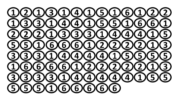
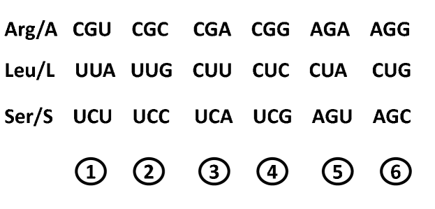
In case it turns out to be difficult to extract the exact positions of the ribosomes from ribosome profiling of such a mRNA strand where the degenerate codons are distributed randomly, we suggest an alternative strategy. Recall that six synonymous codons correspond to the same amino acid Arg; similarly there is six-fold degeneracy also for the amino acids Leu and ser (see fig.14(a)). In principle, one can synthesize an artificial mRNA transcript of the type shown in fig.14(b) using six synonymous codons from any of the three possible sets shown in fig.14(a). A mRNA transcript with such a non-random inhomogeneous codon sequence allows unambiguous identification of the positions of the ribosomes on it while using the ribosome profiling technique ingolia10 .
VI Summary and conclusion
In this paper we have developed a theoretical framework that captures several key features of translation as well as the spatio-temporal organization of polysomes. First, the selection of aa-tRNA in our model is a two-stage process; the second stage captures kinetic proofreading. Second, our model allows occasional translational error and we calculate several quantities as functions of the translational fidelity. We have also incorporated some of the other features of the mechano-chemical cycle of ribosomes in the elongation stage which, to our knowledge, have not been incorporated in any earlier model. On the basis of our hypothesis for capturing the effects of ribosome recycling, we have predicted the effects of recycling on the spatial profile of the ribosomes as well as on the rate of protein synthesis.
Here we have also investigated the spatial organization of ribosomes in polysomes in terms of the distance-headway distribution; it is a quantity that is used extensively to characterize crowding in vehicular traffic. We have also identified the parameter regimes which display distinct characters of polysomes and the corresponding rates of protein production in our model system. Finally, we have also demonstrated the effects of sequence inhomogeneity of the mRNA transcript, particularly, that of the clustering of slow codons.
We hope this work will inspire experimental investigation for measuring new quantities. It is possible to test some of our new predictions using polysome profile techniques. But, more interesting results on spatial distributions of the ribosomes on the mRNA transcript would require ribosome profiling ingolia10 ; guo10 .
Acknowledgements
This work is supported by IIT Kanpur through the Dr. Jag Mohan Chair professorship to one of the authors (DC). DC also thanks the visitors program of the Max-Planck Institute for Physics of Complex Systems for hospitality in Dresden during the preparation of this manuscript.
VII References
References
- (1) N.T. Ingolia, S. Ghaemmaghami, J.R.S. Newman and J.S. Weissman, Genome-wide analysis in vivo of translation with nucleotide resolution using ribosome profiling, Science 324 (2009) 218-223.
- (2) H. Guo, N.T. Ingolia, J.S. Weissman and D.P. Bartel,Mammalian microRNAs predominantly act to decrease target mRNA levels, Nature 466 (2010) 835-840.
- (3) A.K. Sharma and D. Chowdhury, Distribution of dwell times of a ribosome: effects of infidelity, kinetic proofreading and ribosome crowding, Phys. Biol. 8 (2011) 026005
- (4) A. S. Spirin, Ribosomes, Springer (2000).
- (5) A.S. Spirin, Ribosome as a molecular machine, FEBS Lett. 514 (2002) 2-10.
- (6) J. Frank and C.M.T. Spahn, The ribosome and the mechanism of protein synthesis, Rep. Prog. Phys. 69 (2006) 1383-1417.
- (7) J. Frank (ed.), Molecular machines (Cambridge University Press, 2011).
- (8) B. Alberts et al., Essential Cell Biology, Garland Science (2003).
- (9) H. F. Lodish, Model for the regulation of mRNA translation applied to haemoglobin synthesis, Nature 251 (1974) 385-388.
- (10) G. Hirokawa, N. Demeshkina, N. Iwakura, H. Kaji and A. Kaji, The ribosome-recycling step: consensus or controversy? , Trends. Biochem. Sci. 31 (2006) 143-149.
- (11) D. Chowdhury, L. Santen and A. Schadschneider, Statistical physics of vehicular traffic and some related systems Phys. Rep. 329 (2000) 199-329.
- (12) A. Schadschneider, D. Chowdhury and K. Nishinari, Stochastic transport in complex systems: from molecules to vehicles ELSEVIER, Amsterdam, The Netherlands (2010).
- (13) D. Chowdhury, A. Schadschneider and K. Nishinari, Physics of Transport and Traffic Phenomena in Biology: from molecular motors and cells to organisms, Phys. of Life Rev. 2 (2005) 318-352.
- (14) J.R. Warner, A. Rich and C.E. Hall, Electron microscope studies of ribosomal clusters synthesizing hemoglobin Science 138 (1962) 1399-1403.
- (15) J.R. Warner, P.M. Knopf and A. Rich, A multiple ribosomal structure in protein synthesis, PNAS 49 (1963) 122-129.
- (16) A. Rich, The excitement of discovery, Annu. Rev. Biochem. 73 (2004) 1-37.
- (17) H. Noll, The discovery of polyribosomes, Bioessays 30 (2008) 1220-1234.
- (18) A.K. Sharma and D. Chowdhury, Quality control by a mobile molecular workshop: Quality versus quantity, Phys. Rev. E 82 (2010) 031912.
- (19) Y. Arava, Y. Wang, J.D. Storey, C.L. Liu, P.O. Brown and D. Herschlag, Genome-wide analysis of mRNA translation profiles in saccharomyces cerevisiae, PNAS 100 (2003) 3889-3894.
- (20) E. Mikamo, C. Tanaka, T. kanno, H. Akiyama, G. Jung, H. Tanaka and T. Kawai, Native polysomes of Saccharomyces cerevisiae in liquid solution observed by atomic force microscopy, J. Struct. Biol. 151 (2005) 106-110.
- (21) Y. Arava, F. Edward Boas,Patrick O. Brown and Daniel Herschlag, Dissecting eukaryotic translation and its control by ribosome density mapping, Nucl. Acids Res. 33 (2005) 2421-2432.
- (22) Zhdanov, Kinetic models of gene expression including non-coding RNAs, Phys. Rep. 500 (2011) 1-42.
- (23) B. Derrida, Phys. Rep. 301 (1998) 65-83.
- (24) G. M. Schütz, Phase Transitions and Critical Phenomena, vol. 19, Acad. Press (2001).
- (25) D. Mukamel, Phase transitions in nonequilibrium systems, in: Soft and Fragile matter: nonequilibrium dynamics, metastability and flow, eds. M.R. Evans and M.E. Cates (Taylor and Francis, 2000).
- (26) C. MacDonald, J. Gibbs and A. Pipkin, Kinetics of biopolymerization on nucleic acid templates, Biopolymers 6 (1968) 1-25.
- (27) C. MacDonald and J. Gibbs,Concerning the kinetics of polypeptide synthesis on polyribosomes, Biopolymers, 7 (1969) 707-725.
- (28) G. Lakatos and T. Chou, Totally asymmetric exclusion processes with particles of arbitrary size , J. Phys. A 36 (2003) 2027-2041.
- (29) Leah B. Shaw, R.K.P. Zia and Kelvin H Lee, Totally asymmetric exclusion process with extended objects: A model for protein synthesis, PRE 68 (2003) 021910
- (30) L.B. Shaw, J.P. Sethna and K.H. Lee,Mean-field approaches to the totally asymmetric exclusion process with quenched disorder and large particles, Phys. Rev. E 70 (2004) 021901.
- (31) L.B. Shaw, A.B. Kolomeisky and K.H. Lee, Local Inhomogeneity in Asymmetric Simple Exclusion Processes with Extended Objects J. Phys. A 37 (2004) 2105-2113.
- (32) Tom Chou, Ribosome recycling, diffusion, and mRNA loop formation in translational regulation,Biophysical Journal 85 (2003) 755-773.
- (33) T. Chou and G. Lakatos, Clustered Bottlenecks in mRNA Translation and Protein Synthesis, Phys. Rev. Lett. 93 (2004) 198101.
- (34) R.K.P. Zia, J.J. Dong and B. Schmittmann, Modeling Translation in Protein Synthesis with TASEP: A Tutorial and Recent Developments, J. Stat. Phys. (2011), and references therein.
- (35) H. Zouridis and V. Hatzimanikatis, Effects of codon distributions and tRNA competition on protein translation, Biophys. J. 95, (2008) 1018-1033.
- (36) L.M.Y.T. Romero, M. Silber and V. Hatzimanikatis, The origins of time-delay in template biopolymerization processes, PLoS Comp. Biol. 6, (2010) e1000726.
- (37) L. Ciandrini, I. Stansfield and M.C. Romano, Role of the particle’s stepping cycle in an asymmetric exclusion process: A model of mRNA translation, Phys. Rev. E 81 (2010) 051904.
- (38) A. Basu and D. Chowdhury, Traffic of interacting ribosomes: effects of single-machine mechano-chemistry on protein synthesis , Phys. Rev. E 75 (2007) 021902.
- (39) A. Garai, D. Chowdhury, D. Chowdhury and T.V. Ramakrishnan, Stochastic kinetics of ribosomes: Single motor properties and collective behavior, Phys. Rev. E 80 (2009) 011908.
- (40) J. J. Hopfield, Kinetic Proofreading: a new mechanism for reducing errors in biosynthetic process requiring high specificity, Proc. Nat. Acad. Sci. 71 (1974) 4135-4139
- (41) Jacques Ninio, Kinetic amplification of enzyme discrimination, Biochimie 57 (1975) 587-595
- (42) X. Agirrezabala and J. Frank, Elongation in translation as a dynamic interaction among the ribosome, tRNA, and elongation factors EF-G and EF-Tu, Quart. Rev. Biophys. 42 (2009) 159-200.
- (43) N. M. Reynolds, B.A. Lazazzera and M. Ibba, Cellular mechanisms that control mistranslation, Nat. Rev. Microbiol. 8, (2010) 849-856.
- (44) J. Krug, Phys. Rev. Lett. Boundary-induced phase transitions in driven diffusive systems, 67 (1991) 1882-1885.
- (45) V. Popkov and G. Schütz, Steady-state selection in driven diffusive systems with open boundaries, Europhys. Lett. 48 (1999) 257-263.
- (46) J. Hager, J. Krug, V. Popkov and G. Schütz, Minimal current phase and universal boundary layers in driven diffusive systems, Phys. Rev. E 63 (2001) 056110.
- (47) J. Hager, Extremal principle for the steady-state selection in driven lattice gases with open boundaries, Phys. Rev. E 63 (2001) 067103.
- (48) T. Antal and G.M. Schütz, Asymmetric exclusion process with next-nearest-neighbor interaction: Some comments on traffic flow and a nonequilibrium reentrance transition, Phys. Rev. E 62 (2000) 83-93.
- (49) A. B. Kolomeisky, Asymmetric simple exclusion model with local inhomogeneity J.Phys. A. 31 (1998) 1153-1164.
- (50) M.A. Gilchrist and A. Wagner, A model of protein translation including codon bias, nonsense errors, and ribosome recycling, J. Theor. Biol. 239 (2006) 417-434.
- (51) R.C. Thompson, D.B. Dix and J. F. Eccleston, Single turnover kinetic studies of guanosine triphosphate hydrolysis and peptide formation in the elongation factor Tu-dependent binding of aminoacyl-tRNA to Escherichia coli ribosomes, J biol. chem. 255 (1980) 11088-11090.
- (52) K. M. Harrington, I. A. Nazarenko, D.B.Dix, R.C. Thompson and O.C. Ulhenbeck, In vitro analysis of translational rate and accuracy with an unmodified tRNA, Biochemistry 32 (1993) 7617-7622.
Figure Captions
Fig.1: Detailed mechanochemical cycle of Ribosome on its track.
The integer indices label the codons on the mRNA transcript.
Although the same set of transitions are allowed from each codon, only those
from (and to) the codon are shown explicitly.
Fig.2: Phase diagram of ribosome traffic model in the
3-dimensional space spanned by , and .
Fig.3: Same data as in fig.2, except that
plotted from a different perspective.
Fig.4: Phase diagram of ribosome traffic model in the
3-dimensional space spanned by , and .
Fig.5: Same data as in fig.4, except that
plotted from a different perspective.
Fig.6: Projections of several two-dimensional cross sections,
of the three-dimensional phase diagram, plotted in figs.2
and 3, onto the plane. Each
cross section corresponds to a fixed value of .
Fig.7: Projections of several two-dimensional cross sections,
of the three-dimensional phase diagram, plotted in figs.4
and 5, onto the plane. Each
cross section corresponds to a fixed value of .
Fig.8: 2D Phase diagram of TASEP and -TASEP in the
plane in the presence of recycling of ribosomes.
Fig.9: Variation of the average flux and coverage density
with the recycling factor . The green and red curves have the same
values whereas the red and blue curves have the same
values.
Fig.10: Distribution of distance-headways. The lines have
been obtained by using the formula (44) whereas the
discrete data points have been obtained directly from computer simulations.
Fig11: Density profile of ribosomes for single bottleneck.
Fig.12: Density profile of ribosomes for slow sites at
.
Fig.13: Flux variation with for both lattices
(see text for detail).
Fig.14: Codon-sequence suggested for testing our theoretical
predictions.
(a)
(b)
