Magnetic coupling of planets and small bodies with a pulsar wind.

Abstract

Aims. We investigate the electromagnetic interaction of a relativistic stellar wind with a planet or a smaller body in orbit around the star. This may be relevant to objects orbiting a pulsar, such as PSR B1257+12 and PSR B1620-26 that are expected to hold a planetary system, or to pulsars with suspected asteroids or comets.

Methods. We extend the theory of Alfvén wings to relativistic winds.

Results. When the wind is relativistic albeit slower than the total Alfvén speed, a system of electric currents carried by a stationary Alfvénic structure is driven by the planet or by its surroundings. For an Earth-like planet around a ”standard” one second pulsar, the associated current can reach the same magnitude as the Goldreich-Julian current that powers the pulsar’s magnetosphere.

1 Introduction

Precise pulsar timing measurents proved that the pulsars PSR B1257+12 and PSR B1620-26, host planets, at distances of order of an astronomical unit (Wolszczan & Frail (1992), Thorsett et al. (1993)). Moreover, accretion discs are expected to form at some phase of the evolution of neutron stars in a binary system, possibly giving birth to second generation planets. Small bodies, such as planetoids, asteroids or comets may also orbit pulsars and occasionally fall on them.

Circum-pulsar objects move in the centrifugally driven relativistic pulsar wind. The angular velocity $\Omega_{*}$ of a rotating neutron star typically is larger than 10 rad.s^-1. The star behaves like an antenna (Deutsch 1955) emitting by magnetic dipole radiation a power which causes it to lose rotational energy at a rate

$$\dot{E}_{rot}=-M_{I}\Omega_{*}\dot{\Omega}_{*}=4\pi^{2}M_{I}\dot{P}/P^{3},$$ (1)

where $M_{I}\approx(2/5)MR^{2}$ is the neutron star’s moment of inertia (Lyne & Graham-Smith 1998). This power can be compared to the orbital energy of a pulsar planet. Consider, for example, the case of PSR B1257+12 and its planet ”a”. Using the data in Tables 1 and 2, we can estimate the moment of inertia to be $M_{I}=1.\times 10^{38}$ kg.m², the star’s rotational energy loss to be $\dot{E}_{rot}=-2.\times 10^{27}$ W, and the planet’s orbital energy to be $E_{G}={GM_{*}M_{P}}/{2a}=4.\times 10^{32}$ J, where $a$ stands for the planet’s semi-major axis . The planet and its environment intercept a fraction larger than or of order of $\pi R_{P}^{2}/(4\pi a^{2})$ of this power. This captured power is used to heat the planet, to generate the current system described below and to work on the planet’s motion as described in the accompanying paper (Mottez & Heyvaerts 2011), hereafter (MH2). The planet’s radius can be infered from its mass by assuming a terrestrial density (5000 kg m^-3). The intercepted power ${\dot{E}}_{capt}$ is :

$${\dot{E}}_{capt}={\dot{E}_{rot}}\left(\frac{R_{P}}{2a}\right)^{2}.$$ (2)

For planet ”a” of PSR B1257+12, we find, ${\dot{E}}_{capt}=$ 1.74 10¹⁸ Watts. If a substantial part of this power goes into performing work on the planet’s motion, an orbital evolution time scale of about 8. 10⁶ years may be expected. This is a short time scale by astronomical standards. It scales with the mass $M_{P}$ of the planet as $M_{P}^{1/3}$.

In this paper, we examine the interaction of these planets with the magnetized wind of their pulsar and discuss in (MH2) the effect of this interaction on the long term evolution of their orbital elements.

The energy flux carried by the wind of an ordinary star, such as the Sun, is small enough to have but negligible effect on the orbits of its planets. Stellar winds usually are asymptotically super-Alfvénic, by which we mean that they eventually become faster than the total Alfvén speed, associated with the modulus of the magnetic field. As a result, the planets are protected from a direct contact with the wind by a bow shock.

Pulsar winds are much different. In a first approximation, oblique rotator pulsars may be regarded as magnetic dipoles rotating at high angular velocity in vacuo, which causes a low frequency and large amplitude electromagnetic wave to be emitted, the wave character of which reveals itself in the wave zone, beyond the light cylinder, of radius $r=c/\Omega_{*}$. In this zone, magnetic field lines become spiral-shaped and the azimuthal component of the magnetic field decreases as $B_{\phi}\sim r^{-1}$ while its radial component decreases as $B_{r}\sim r^{-2}$. The magnetic field becomes mostly azimuthal at large distances and at the equatorial latitudes were the planets are expected to be found. Aligned rotators essentially are rotating unipolar inductors which generate, beyond the light cylinder, an highly relativistic MHD wind in which the magnetic field also becomes predominantly azimuthal at large distances from the rotation axis, the field components $B_{\phi}$ and $B_{r}$ varying with distance essentially as indicated above, at least near the equatorial plane and when the flow is close to being radial. The power emitted by such objects is also of order of $\dot{E}_{rot}$, given by Eq. (1), because the Poynting flux emitted through the light cylinder is comparable for wind or wave emission. We only consider aligned rotators in this paper. Their analysis is simplified by the fact that the magnetic field of the wind observed in the planet’s frame is close to being time-independent. The origin, acceleration and structure of pulsar winds are not fully understood. A number of models have been proposed in the literature (Michel 1969; Henriksen & Rayburn 1971; Contopoulos et al. 1999; Michel 2005; Bucciantini et al. 2006). In spite of their diversity, they all converge on the fact that the wind is dominated by the Poynting flux, although observations indicate that they turn into matter-dominated high energy flows at large distances (Kirk et al. 2009). At distances of order of an astronomical unit, pulsar winds are expected to be still Poynting-flux-dominated. This means that the electromagnetic energy density $\sim B_{0}^{2}/\mu_{0}$, $\mu_{0}$ being the magnetic permeability of vacuum, is much larger than the plasma energy density $\gamma_{0}\rho_{0}c^{2}$, $\gamma_{0}$ being its Lorentz factor and $\rho_{0}$ the rest mass density of this supposedly cold wind. These quantities refer to the observer’s frame. In such circumstances, Alfvénic perturbations propagate at a phase velocity close to the speed of light (equation (3)). Therefore, in spite of being highly relativistic, the wind flow may nevertheless be sub-Alfvénic, in the sense defined above. A planet in a Poynting-flux-dominated wind may remain unscreened from the wind by a bow shock and thus enter in direct contact with it.

The interaction of a planet with a sub-Alfvénic plasma flow has been considered for moderately magnetized non-relativistic flows in connection with the interaction of the satellite Io with the plasma and magnetic field present in Jupiter’s magnetospheric environment. This interaction is driven by the inductive electromotive field which results from the motion of the satellite across Jupiter’s corotational magnetic field and plasma flow. The satellite acts as a (uniformly moving) unipolar inductor. Neubauer (1980) derived a nonlinear theory of this interaction. The Alfvén wing connecting Io and Jupiter is the only explored case of such a structure in the universe up to now, and it has been the object of recent studies concerning its overall structure (Chust et al. 2005; Hess et al. 2010), the possibility of particle acceleration (Hess et al. 2007b, 2009b) and its consequences on the radio emissions (Queinnec & Zarka 1998; Hess et al. 2007a, 2009a). In the present paper, we develop a theory that generalizes some of Neubauer’s results to the case of highly magnetized ($B_{0}^{2}>>\mu_{0}\rho_{0}\gamma_{0}c^{2}$) and relativistic plasma flows with Lorentz factors $\gamma_{0}>>1$, when a planet immersed in the magnetized pulsar wind acts as a unipolar inductor and generates two stationary Alfvénic structures that emerge from the planet and extend far in the wind.

2 A unipolar inductor in the pulsar wind

Let us consider a planet orbiting a pulsar in the relativistic flow of the emitted wind. Different reference frames can be involved in the description of the fluid motion. The frame where the neutron star is at rest is the observer’s frame. We denote it by $R_{O}$. The planet velocity being small compared to the wind velocity, we may consider the planet to be at rest with respect to the neutron star, except when discussing the planet’s motion. The reference frame $R_{O}$ can then also be regarded as being the planet’s rest frame. Quantities observed in this frame are denoted by letters without any superscript, such as $\rho$ or ${\mathbf{v}}$. The unperturbed wind’s instantaneous rest frame in the vicinity of the planet is the ”wind’s frame” $R_{W}$. Quantities observed in this frame are denoted by letters with a prime superscript, such as $\rho^{\prime}$. An index $0$ refers to quantities associated with the unperturbed wind. The unperturbed wind velocity in $R_{O}$ is ${\mathbf{v}}_{0}$, its associated Lorentz factor is $\gamma_{0}$, the unperturbed magnetic field is ${\mathbf{B}}_{0}$ and the wind’s density is $\rho_{0}$. The wind plasma being supposedly cold, this mass density reduces to the (apparent) rest mass density of particles. In the wind frame $R_{W}$, the unperturbed wind density is its proper rest mass density $\rho^{\prime}_{0}$ and its magnetic field is ${\mathbf{B}}^{\prime}_{0}$. They both differ from $\rho_{0}$ and ${\mathbf{B}}_{0}$. In the presence of a perturbation, the instantaneous rest frame of the fluid is not $R_{W}$ but another rest frame, $R_{F}$. Quantities observed in this instantaneous rest frame are indicated by a subscript $F$.

The perturbation generated by the planet in this flow is time-dependent in the wind’s frame. Since in the tenuous and highly magnetized pulsar wind the formal Alfvén velocity $c_{A}$ may exceed the speed of light, the derivation of the propagation velocity $V^{\prime}_{A}$ of Alfvénic perturbations must take into account the displacement current. In the wind’s rest frame :

$$V_{A}^{{}^{\prime}-2}=c^{-2}+c_{A}^{{}^{\prime}-2}=c^{-2}+\mu_{0}\rho^{\prime}_{0}/{B^{\prime}_{0}}^{2}.$$ (3)

If the flow is faster than the Alfvén velocity $V_{A}$, the planet is preceded by a shock wave that defines a confined area where the flow is strongly modified. But if the flow is sub-Alfvénic, the planet is directly in contact with the wind. In the instantaneous rest frame of the wind plasma we expect, following the MHD approximation, the electric field to vanish. In the planet’s rest frame an electromotive field ${\bf E}=-{\bf v}\times{\bf B}$ is generated, where ${\bf B}$ and ${\bf v}$ are the magnetic field and fluid velocity in the planet’s frame.

Using a model pulsar wind, it is possible to make an estimate of the electric field. One of the simplest such models was developed by Michel (1969). It includes the magnetic field and the star’s rotation, wind particles masses, but neglects the dipole inclination and the gravitation and assumes the wind flow to be radial. The unperturbed magnetic field ${\mathbf{B}}_{0}$ only has a radial poloidal component $B_{0}^{r}$ and an azimuthal toroidal component $B_{0}^{\phi}$. The neglect of the latitudinal component $B_{0}^{\theta}=0$ is justified near the equatorial plane and far enough from the inner magnetosphere (Contopoulos et al. 1999). For bodies orbiting near this plane, as circumpulsar planets probably do, this geometrical restriction is unimportant. Other models for steady state axisymmetric winds have been developed since then (Beskin et al. 1998; Bucciantini et al. 2006). The stationary equations of an axisymmetric perfect MHD flow admit a set of integrals of motion along stream lines, such as the mass flux $f$ and the magnetic flux $\Psi$, which, for cold radial flows and radial poloïdal fields, are defined by:

$$f = \gamma_{0}\rho^{\prime}_{0}v_{O}^{r}r^{2},$$ (4)

$$\Psi = r^{2}B_{0}^{r},$$ (5)

where all quantities refer to the unperturbed wind as seen in the observer’s frame. The MHD approximation ${\bf E}_{0}+{\bf v}_{0}\times{\bf B}_{0}=0$ and the Faraday equation imply (Mestel 1961):

$$B_{0}^{\phi}=B_{0}^{r}\frac{v_{0}^{\phi}-\Omega_{*}r}{v_{0}^{r}}.$$ (6)

In order to judge whether the planet is in superalfvénic motion with respect to the wind, we should assess whether the modulus of its velocity in the wind’s frame, which equals that of the wind in the observer’s frame, $v_{0}$, is faster or not than the propagation speed in the wind’s frame, $V^{\prime}_{A}$, defined by Eq. (3). The square of the ratio of these two velocities is given, for an asymptotically radial wind, by :

$${M^{\prime}_{A}}^{2}=\left(\frac{v_{0}^{r}}{V^{\prime}_{A}}\right)^{2}=\left(\frac{v_{0}^{r}}{c}\right)^{2}\left(1+\frac{c^{2}}{{c^{\prime}_{A}}^{2}}\right).$$ (7)

The wind being supposedly radial, $v_{0}^{\phi}$ vanishes. This simplifies equation (6) which also shows that at distances much larger than the light cylinder radius, the radial component of the magnetic field can be neglected compared to the azimuthal one. The Alfvén speed $c_{A}$ calculated in the observer’s frame is given, using equations (4) and (5) to express $B_{0}^{r}$ and $\rho^{0}$, by:

$$\frac{c_{A}^{2}}{c^{2}}=\frac{\Omega_{*}^{2}\Psi^{2}}{\mu_{0}fc^{3}}\ \frac{c}{v_{0}^{r}}.$$ (8)

The square of the Alfvén speed $c^{\prime}_{A}$ in the wind’s frame is a factor $\gamma_{0}$ smaller than the square of the Alfvén speed $c_{A}$ in the observer’s frame because $\rho_{0}=\gamma_{0}\rho^{\prime}_{0}$ and $B_{\phi 0}=\gamma_{0}B^{\prime}_{\phi 0}$. The latter relation is a result of the vanishing of the electric field in the wind’s frame and of the velocity ${\mathbf{v}}_{0}$ being perpendicular to the azimuthal field. Then:

$${M^{\prime}_{A}}^{2}=\left(\frac{v_{0}^{r}}{c}\right)^{2}\left[1+\frac{\gamma_{0}}{\sigma_{0}}\left(\frac{v_{0}^{r}}{c}\right)\right],$$ (9)

where $\sigma_{0}$ is the magnetization parameter:

$$\sigma_{0}=\frac{\Omega_{*}^{2}\Psi^{2}}{\mu_{0}fc^{3}}.$$ (10)

In highly relativistic Poynting-flux-dominated outflows, as is expected for pulsar winds, $\sigma_{0}\gg 1$. The models show that asymptotically the Lorentz factor $\gamma_{0}$ approaches $\sigma_{0}^{1/3}$ and thus $(v_{0}/c)^{2}$ approaches $(1-\sigma_{0}^{-2/3})$. From equation (9), it is found that, to lowest order in an expansion in $\sigma_{0}^{-1}$, the asymptotic value of ${M^{\prime}_{A}}$ is $(1-1/(2\sigma_{0}^{4/3}))$. Therefore the pulsar wind remains slower than the total Alfvén speed (3).

Since this result applies at distances much larger than the light cylinder radius, it is essentially valid wherever planets may be found orbiting. We therefore consider that the planets detected around pulsars orbit in a sub-Alfvénic relativistic pulsar wind.

In the numerical computations, we are less subtle and state that at the planetary distances, $v_{0}\sim c$ and $V_{A}\sim c$, every time it makes sense. Then, in first approximation, the unipolar inductor electric potential drop $U$ (along the $\theta$ axis, i.e. perpendicular to the orbital plane) is

$$U=2R_{P}E_{0}=2R_{P}E_{0}^{\theta}=2R_{P}v_{0}^{r}B_{0}^{\phi}=\frac{2R_{P}\Omega_{*}\Psi}{r}.$$ (11)

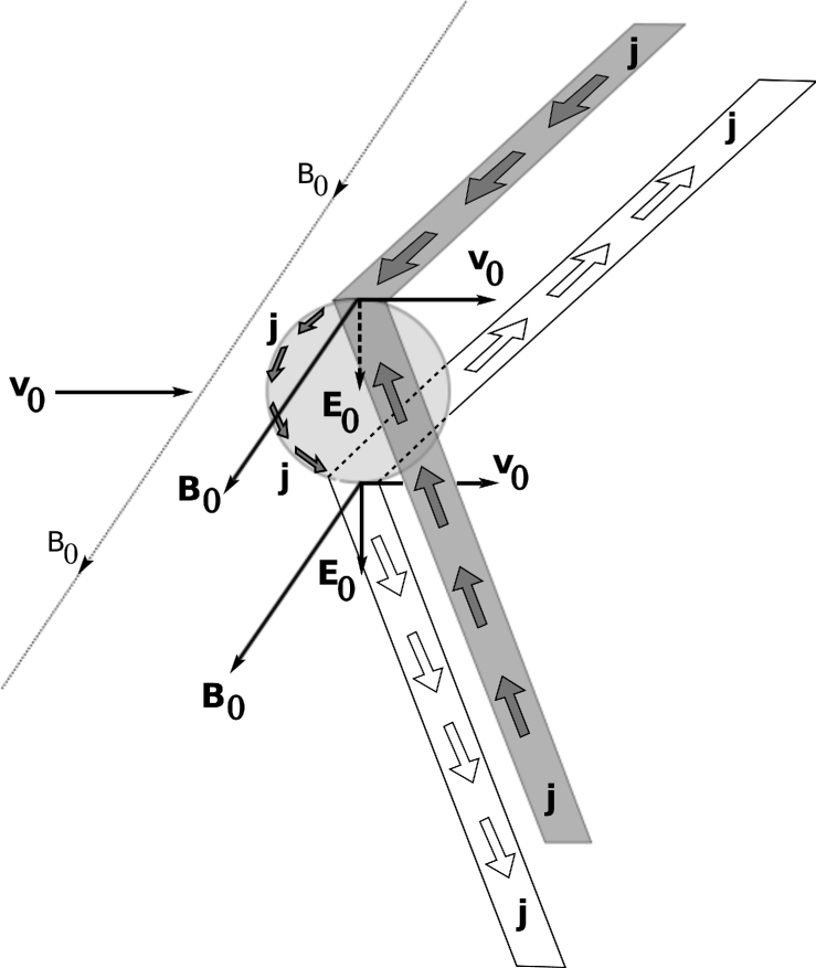
Figure 1: Schematic view of an unipolar inductor.

The Fig. 1 provides a representation of the geometric configuration of the unipolar inductor.

The rotation period of the pulsar PSR 1257+12 is $P=0,006$s, which corresponds to $\Omega_{*}$ = 1010,397 rad.s^-1 and its surface magnetic field is estimated to $B_{*}\simeq 8.8\times 10^{8}$G (Taylor et al. 2000). We assume a star radius $R_{*}=10$ km and a mass $M_{*}=1.4M_{\odot}$ (see Table 1). Data concerning this planet can be read in table 2. We assume an Earth-like density of 5000 kg.m^-3. The flux $\Psi=R_{*}^{2}B_{*}=8.8\times 10^{12}$ Wb. The semi-major axis, the planetary radius $R_{P}=(3M_{P}/4\pi\rho_{P})^{1/3}$ and an estimate of $U$ are given for each planet ”a”, ”b”, ”c” orbiting this pulsar in Tables 2 and 3. It can be seen that the inductor electric potential drop $U$ (from pole to pole along the planet) is of the order of $10^{12}$ V.

For the pulsar PSR 1620-26, the rotation period is $P=0,011$s, $\Omega_{*}$ = 567 rad.s^-1, the surface magnetic field is estimated to $B_{*}=3.\times 10^{9}$G (Taylor et al. 2000). Still assuming that $R_{*}=10$ km, we find that $\Psi=3\times 10^{13}$ Wb. This pulsar has a white dwarf companion star. The neutron star mass can be estimated to $M_{*}=1.35M_{\odot}$ (Thorsett & Arzoumanian 1999; Sigurdsson et al. 2003). The planet is more distant from its star than in the case of PSR 1257+12 but the planetary radius is larger. The resulting potential drop $U$ is still of the same order of magnitude.

We show in sections 3–5 that a planet in the wind generates two current systems that propagate far in space, forming a so-called Alfvén wing.

3 Equations of special-relativistic ideal MHD

In this section, the equations up to Eq. (23) are general to special relativity, and valid for quantities defined in any inertial reference frame. We use notations without prime and subscript. After Eq. (23), quantities without prime and subscript refer, as in the previous sections, only to the observer’s frame $R_{O}$ defined at the begining of section 2.

A condition for MHD to be valid is that the typical length scale $L$ relevant to the flow be much larger than the particles Larmor radii $\rho_{L}=\gamma v_{\perp}/\omega_{c}$, where $v_{\perp}$ is the typical velocity perpendicular to the magnetic field in the fluid’s frame, $\omega_{c}$ the gyrofrequency and $\gamma$ the particle’s Lorentz factor in the same frame. The energy of particles in a pulsar wind is a priori very high since the wind’s bulk Lorentz factor $\gamma_{0}$ may be as large as $10^{5}$ to $10^{7}$. If however, in the wind’s frame, a significant part of this energy resided in perpendicular motions, particles would very quickly loose it by synchrotron radiation, even in a moderate magnetic field. Therefore, we may consider the pulsar wind particles to have negligible Larmor radii in the rest frame of the wind’s bulk flow, so that MHD is applicable on almost any scale.

The fourth component of position in space time is $x^{4}=ct$, $t$ being the time measured in seconds in the given reference frame and $c$ the speed of light. Greek indices label four-dimensional coordinates and components and latin indices label Euclidean three-dimensional ones. The metric tensor of Minkowskian space is diagonal, with components $\eta_{44}=+1$ and $\eta_{11}=\eta_{22}=\eta_{33}=-1$. $\nabla_{\mu}$ designates the partial derivative with respect to the space-time coordinate $x^{\mu}$. The notation ${\boldsymbol{\nabla}}$ designates the three-dimensional nabla operator. We use the dummy index rule. Special-relativistic MHD equations associate fluid equations with Maxwell’s equations, in which the displacement current and Poisson’s equation should be retained. The fluid equations consist of a conservation equation for particle number, valid in the absence of reactions among particle species, and of the four components of the energy and momentum conservation equations The law of conservation of particle number is written as:

$$\nabla_{\mu}(n_{F}\,u^{\mu})=0\,.$$ (12)

The density $n_{F}$ is the proper spatial number density of particles, that is, their density measured in the instantaneous rest frame of the fluid. The four components $u^{\mu}$ are those of the dimensionless four-velocity of the fluid in the considered rest frame:

$$u^{\mu}=(\gamma\,{{\bf v}}/c\,,\,\gamma)\,.$$ (13)

The Lorentz factor $\gamma$ refers here to the bulk fluid motion. The number density in the observer’s frame is the fourth component of the density-flux four-vector, $n_{F}\gamma$. The equations of conservation of energy and momentum of matter are lumped in the four-tensorial equation:

$$\nabla_{\mu}T_{m}^{\mu\nu}=f_{em}^{\nu}\,.$$ (14)

The $T_{m}^{\mu\nu}$’s are the components of the energy-momentum tensor of matter and the components $f_{em}^{\nu}$ are those of the electromagnetic force density four-vector. By using Maxwell’s equations, this four-vector can be written in conservative form and equation (14) can be given the form:

$$\nabla_{\mu}(T_{m}^{\mu\nu}+T_{em}^{\mu\nu})=0\,.$$ (15)

The $T_{em}^{\mu\nu}$’s are the components of the electromagnetic energy-momentum tensor. They can be expressed in terms of the electromagnetic field strength tensor $F$ or in terms of the electric and magnetic fields observed in the chosen reference frame. Its time-time component is the electromagnetic energy density, its space-time components are the three components of the Poynting vector divided by $c$ and its space-space components form a second rank tensor of the three-dimensional Euclidean space, the Maxwell stress tensor:

$${\overline{\overline{\mathbf{M}}}}=\left(\frac{\varepsilon_{o}E^{2}}{2}+\frac{B^{2}}{2\mu_{0}}\right)\,{\overline{\overline{\boldsymbol{\delta}}}}-\varepsilon_{o}{\overline{\overline{{\mathbf{E}}{\mathbf{E}}}}}-\frac{{\overline{\overline{{\mathbf{B}}{\mathbf{B}}}}}}{\mu_{0}}\,.$$ (16)

The symbol $\boldsymbol{\delta}$ represents the second rank unit tensor. The matter energy-momentum tensor of a cold pressureless fluid can be written, in the absence of non-ideal effects such as viscosity, as:

$$T_{m}^{\mu\nu}=\rho_{F}c^{2}u^{\mu}u^{\nu}\,.$$ (17)

In the absence of internal heat, the number conservation equation (12) reduces to a conservation equation for proper mass, since in this case $\rho_{F}=m\,n_{F}$, $m$ being the rest mass of particles. Equation (12) can then be written in three-dimensional notations as:

$$\frac{\partial\,\gamma\rho_{F}}{\partial t}+{\mathrm{div}}\,(\gamma\rho_{F}{{\bf v}})=0\,.$$ (18)

Here, we need not solve the energy conservation equation because the medium is regarded as cold. We only consider the spatial components of the equivalent equations (14) or (15). From equation (14) we get, denoting the charge and current density by $\rho_{e}$ and ${\mathbf{j}}$ respectively:

$$\frac{\partial}{\partial t}\left(\gamma^{2}\rho_{F}\,{\mathbf{v}}\right)+{\mathrm{div}}\,\left(\gamma^{2}\rho_{F}\,{\overline{\overline{{\mathbf{v}}{\mathbf{v}}}}}\right)=\rho_{e}{\mathbf{E}}+{\mathbf{j}}\times{\mathbf{B}}\,.$$ (19)

From equation (15) we get the equivalent equation:

$$\frac{\partial}{\partial t}\left(\gamma^{2}\rho_{F}\,{\mathbf{v}}+\frac{{\mathbf{E}}\times{\mathbf{B}}}{\mu_{0}c^{2}}\right)+{\mathrm{div}}\,\left(\gamma^{2}\rho_{F}\,{\overline{\overline{{\mathbf{v}}{\mathbf{v}}}}}+{\overline{\overline{\mathbf{M}}}}\right)=0\,.$$ (20)

The components of the Maxwell stress tensor ${\overline{\overline{\mathbf{M}}}}$ may be transformed to account for the perfect MHD relation

$${\mathbf{E}}+{\mathbf{v}}\times{\mathbf{B}}=0\,.$$ (21)

The components of the electric field and those of the Maxwell stress tensor are easily calculated in a frame where the $x$-axis is taken to be along the direction of the fluid velocity ${\mathbf{v}}$. Some algebra then yields the following expression, where the indices $t$ (transverse) and $l$ (longitudinal) refer to a component of a vector perpendicular or parallel to the velocity ${\mathbf{v}}$ of the fluid:

$${\overline{\overline{\mathbf{M}}}}=\frac{B_{l}^{2}}{2\mu_{0}}\ {\overline{\overline{\boldsymbol{\delta}}}}+\frac{1}{\gamma^{2}}\frac{B_{t}^{2}}{2\mu_{0}}\ {\overline{\overline{\boldsymbol{\delta}}}}-\frac{{\overline{\overline{{\mathbf{B}}{\mathbf{B}}}}}}{\mu_{0}}+\frac{B_{t}^{2}}{\mu_{0}}\,\frac{{\overline{\overline{{\mathbf{v}}{\mathbf{v}}}}}}{c^{2}}+\frac{v^{2}}{c^{2}}\,\frac{{\overline{\overline{{\mathbf{B}}_{t}{\mathbf{B}}_{t}}}}}{\mu_{0}}\,.$$ (22)

The magnetic field evolution equation, deduced from Faraday’s equation and the perfect MHD relation, writes:

$$\frac{\partial{{\bf B}}}{\partial t}={\mathrm{curl}}({{\bf v}}\times{{\bf B}})\,.$$ (23)

The non-relativistic theory of Neubauer (1980) considers only the Alfvénic wake of the satellite. Indeed, fast MHD disturbances propagate isotropically in the low-$\beta_{P}$ limit and decrease in amplitude with distance from the source ($\beta_{P}$ is the ratio of the plasma pressure to the magnetic pressure). Such disturbances do not create any concentrated current system. The slow mode propagates in a low-$\beta_{P}$ plasma much slower than Alfénic perturbations and the associated disturbances, though channelled by the magnetic field, soon become spatially separated from the Alfénic wake. Actually, slow mode perturbations barely propagate at all in a cold pulsar wind and carry negligible current. The effects of compressive perturbations in the non-relativistic situation have been discussed by Wright & Schwartz (1990) who have shown that compressive plasma wave modes, though necessarily excited, contribute one order of magnitude less to the current flow and to the energy budget than shear Alfvén perturbations do. We therefore follow Neubauer in concentrating on purely Alfvénic motions. We assume that the fluid motions triggered when the planet passes by are sub-relativistic in the rest frame $R_{W}$ of the unperturbed wind and that the changes of the formal Alfvén velocity are similarly sub-relativistic. We do not assume however that the formal Alfvén speed calculated from the total field, $B^{\prime}/(\mu_{0}\rho^{\prime})^{1/2}$, is less than the speed of light. Our assumption of non-relativistic Alfvénic motions in $R_{W}$ implies that ${\mathrm{div}}\,{{\bf v}}^{\prime}=0$. It does not follow however that the same relation also holds true in the observer’s frame $R_{O}$ because the wind flow is relativistic in this frame. In $R_{W}$, the electric terms of the Maxwell stress tensor are by of order $v^{\prime 2}/c^{2}$ less than the magnetic terms and can be neglected. Accounting for the relation ${\mathrm{div}}\,{{\bf v}}^{\prime}=0$, equation (23) can be written as:

$$\frac{d{\mathbf{B}}^{\prime}}{dt^{\prime}}-\left({\mathbf{B}}^{\prime}\cdot{\boldsymbol{\nabla}}^{\prime}\right){\mathbf{v}}^{\prime}=0\,.$$ (24)

Considering Eqs. (21) and (22), the equation of motion (20) becomes, in $R_{W}$,

$$\frac{\mathrm{d}}{{\mathrm{d}}t^{\prime}} \left(\rho^{\prime}{\mathbf{v}^{\prime}}+\frac{B^{\prime 2}{\mathbf{v}^{\prime}}}{\mu_{o}c^{2}}-\frac{({\mathbf{v}^{\prime}}\cdot{\mathbf{B}^{\prime}})\,{\mathbf{B}^{\prime}}}{\mu_{o}c^{2}}\right)$$ (25)

$$-\Big{(}{\mathbf{B}^{\prime}}\cdot{\boldsymbol{\nabla}^{\prime}}\Big{)}\left(\frac{{\mathbf{B}^{\prime}}}{\mu_{o}}+\frac{({\mathbf{v}^{\prime}}\cdot{\mathbf{B}^{\prime}})\,{\mathbf{v}^{\prime}}}{\mu_{o}c^{2}}\!\right)=0.$$

4 An Alfvénic first integral

The computation of the non relativistic Alfvén wing given by Neubauer (1980) is based upon the fact that, in simple non-linear Alfvénic wave motions, the velocity ${\bf V}_{s}={\bf v}-s\ {\bf c}_{A}$ is a first integral. In this relation, ${\mathbf{v}}$ is the fluid’s velocity, ${\bf c}_{A}$ the vectorial Alfvén velocity associated with the perturbed field, and the sign $s=\pm 1$ depends on the sense of propagation of the perturbation. This relation can be transposed in a differential form as $d{\bf B}=kd{\bf v}$, where $k=(\mu_{0}\rho)^{1/2}$. Moreover, the modulus of the magnetic field is a time invariant and, because of the uniform boundary conditions $B=B_{0}$, this modulus is constant over the whole space.

As Neubauer, we look for a solution where $d{\bf B}^{\prime}=kd{\bf v}^{\prime}$ and where $B^{\prime}$ is constant. Then, setting ${\bf b}^{\prime}={\bf B}^{\prime}/B^{\prime}$ and

$$\lambda=(\mu_{0}\rho^{\prime}+B^{\prime 2}/c^{2})^{1/2},$$ (26)

we can write the Eqs. (24) and (25) in the form

$$\lambda^{2}\frac{{d}{\bf v}^{\prime}}{{{d}}t^{\prime}}\!-B^{\prime 2}({\bf b}^{\prime}\cdot\nabla^{\prime}){\bf b}^{\prime}\!-\!\frac{B^{\prime 2}}{c^{2}}\left[\frac{dv^{\prime}_{\parallel}{\bf b}^{\prime}}{dt^{\prime}}\!+\!({\bf b}^{\prime}\cdot\nabla^{\prime})(v^{\prime}_{\parallel}{\bf v}^{\prime})\right]\!=0$$ (27)

$$\frac{d{\mathbf{b}}^{\prime}}{dt^{\prime}}-({\mathbf{b}}^{\prime}\cdot{\boldsymbol{\nabla}}^{\prime}){\mathbf{v}}^{\prime}=0,$$ (28)

where $v^{\prime}_{\parallel}={\bf v}^{\prime}\cdot{\bf b}^{\prime}$. The two first terms of Eq. (27) are analogous to those of classical MHD, when $V_{A}<<c$. The two others are specific to fast variations of the electric field, when the displacement current is taken into account. We solve this system in the following way: we first ignore the last two terms of Eq. (27) and solve the resulting system (27)–(28), which can then be written as:

$$\lambda^{2}\frac{\mathrm{d}{\bf v}^{\prime}}{{\mathrm{d}}t^{\prime}}-B^{\prime 2}({\bf b}^{\prime}\cdot\nabla^{\prime}){\bf b}^{\prime}=0,$$ (29)

$$\frac{d{\mathbf{b}}^{\prime}}{dt^{\prime}}-({\mathbf{b}}^{\prime}\cdot{\boldsymbol{\nabla}}^{\prime}){\mathbf{v}}^{\prime}=0.$$ (30)

We then check whether the last two terms in Eq. (27) vanish or are negligible. These terms are:

$$\frac{B^{\prime 2}}{c^{2}}\left[\frac{dv^{\prime}_{\parallel}{\bf b}^{\prime}}{dt^{\prime}}+({\bf b}^{\prime}\cdot\nabla^{\prime})(v^{\prime}_{\parallel}{\bf v}^{\prime})\right]\,.$$ (31)

Considering Eqs. (29) and (30), the proportionality of $d{\bf B}^{\prime}$ and $d{\bf v}^{\prime}$ is obtained for $k=s\lambda$, and these two equations become equivalent to

$$B^{\prime}d{\bf b}^{\prime}=s\lambda d{\bf v}^{\prime}$$ (32)

$$s\lambda\frac{d{\mathbf{b}}^{\prime}}{dt^{\prime}}-B^{\prime}({\bf b}^{\prime}\cdot\nabla^{\prime}){\bf b}^{\prime}=0.$$ (33)

Eq. (32) has a first integral ${\bf V}^{\prime}_{s}$,

$${\bf V}^{\prime}_{s}={\bf v}^{\prime}-s\,\frac{{\bf B}^{\prime}}{(\mu_{0}\rho^{\prime}+B^{\prime 2}/c^{2})^{1/2}}.$$ (34)

In the region not perturbed by the planet, ${\bf v}^{\prime}=0$, and ${\bf B}^{\prime}={\bf B}^{\prime}_{0}$. Therefore,

$${\bf V}^{\prime}_{s}=-s\frac{{\bf B}^{\prime}_{0}}{\lambda},$$ (35)

$${\bf v}^{\prime}=\frac{s}{\lambda}({\bf B}^{\prime}-{\bf B}^{\prime}_{0}),$$ (36)

$$v^{\prime}_{\parallel}=\frac{s}{\lambda}(B^{\prime}-{\bf b}^{\prime}\cdot{\bf B}^{\prime}_{0}).$$ (37)

In order of magnitude, $\lambda\sim B^{\prime}/c$, and the approximation $v^{\prime}<<c$ implies that $\|{\bf B}^{\prime}-{\bf B}^{\prime}_{0}\|<<B^{\prime}_{0}$. Therefore, this is equivalent to an hypothesis of linear perturbation. This remark also holds for the computations of Neubauer (1980). At this stage, it is necessary to evaluate the terms in Eq. (31). Using the above relations, these terms are

$$-s\,\frac{B^{\prime 2}}{c}\left(\frac{d{\bf b}^{\prime}}{dt^{\prime}}\cdot\frac{{\bf v}^{\prime}}{c}\right){\bf b}^{\prime}_{0}\,,$$ (38)

where ${\bf b}^{\prime}_{0}$ is the direction of the unperturbed magnetic field in the wind’s frame of reference. The quantity in Eq. (38) does not vanish but it is negligible, as long as $v^{\prime}<<c$, in comparison to the terms in Eq. (29), which are of the order of $(B^{\prime 2}/c)d{\bf b}^{\prime}/dt^{\prime}$. Therefore, in the linear approximation, the solution given by Eqs. (32-37) is correct.

The first integral of Eq. (34) must now be computed in the observer’s frame of reference $R_{O}$. It will be used in the next section to derive the value of the electric current associated to the Alfvén wings. Let us write the velocity and the magnetic field as the sum of a longitudinal component, parallel to ${\bf v}_{0}$, and a transverse vector component.

$${{\bf B}}_{l} = \frac{{\overline{\overline{{{\bf v}}_{0}{{\bf v}}_{0}}}}}{v_{0}^{2}}\cdot{{\bf B}},$$ (39)

$${{\bf B}}_{t} = \,\left({\overline{\overline{\boldsymbol{\delta}}}}-\frac{{\overline{\overline{{{\bf v}}_{0}{{\bf v}}_{0}}}}}{v_{0}^{2}}\right)\cdot{{\bf B}}.$$ (40)

The transforms of the velocity and of the magnetic field are

$${\mathbf{v}}^{\prime} = \frac{{\mathbf{v}}_{l}-{\mathbf{v}}_{0}+{\mathbf{v}}_{t}/\gamma_{0}}{1-{{\mathbf{v}}\cdot{\mathbf{v}}_{0}}/{c^{2}}},$$ (41)

$${\mathbf{B}}_{l}^{\prime} = {\mathbf{B}}_{l},$$ (42)

$${\mathbf{B}}_{t}^{\prime} = \gamma_{0}\left({\mathbf{B}}_{t}\left(1-\frac{{\mathbf{v}}\cdot{\mathbf{v}}_{0}}{c^{2}}\right)+\frac{{\mathbf{B}}\cdot{\mathbf{v}}_{0}}{c^{2}}{\mathbf{v}}_{t}\right),$$ (43)

where $\gamma_{0}$ is the Lorentz factor of the unperturbed wind. For the transform of the magnetic field, Eq. (21) has been taken into account. The Eq. (34) becomes

$${\mathbf{V}}^{\prime}_{s} = \frac{{\mathbf{v}}_{l}-{\mathbf{v}}_{0}+{\mathbf{v}}_{t}/\gamma_{0}}{1-\frac{{\mathbf{v}}\cdot{\mathbf{v}}_{0}}{c^{2}}}$$ (44)

$$-\,\frac{s}{\lambda}\,\left(\gamma_{0}\left({\mathbf{B}}_{t}\left(1-\frac{{\mathbf{v}}\cdot{\mathbf{v}}_{0}}{c^{2}}\right)+\frac{{\mathbf{B}}\cdot{\mathbf{v}}_{0}}{c^{2}}\,{\mathbf{v}}_{t}\right)+{\mathbf{B}}_{l}\right).$$

For a first order development, we note ${\mathbf{v}_{1}}$ the velocity perturbation and ${\mathbf{B}_{1}}$ the magnetic perturbation,

$${\mathbf{v}}={\mathbf{v}}_{0}+{\mathbf{v}_{1}}\qquad\qquad{\mathbf{B}}={\mathbf{B}}_{0}+{\mathbf{B}_{1}}.$$ (45)

To the first order, Eq. (44) becomes

$${\mathbf{V}}^{\prime}_{s}\ = \gamma_{0}^{2}\left({\mathbf{v}}_{1l}+\frac{{\mathbf{v}}_{1t}}{\gamma_{0}}\right)-\,\frac{s}{\lambda}\left({\mathbf{B}}_{0l}+{\mathbf{B}}_{1l}\right)$$ (46)

$$- \ \frac{s\gamma_{0}}{\lambda}\ \left(\frac{1}{\gamma_{0}^{2}}\left({\mathbf{B}}_{0t}+{\mathbf{B}}_{1t}\right)-{\mathbf{B}}_{0t}\frac{{\mathbf{v}}_{0}\cdot{\mathbf{v}_{1}}}{c^{2}}+\frac{{\mathbf{B}}_{0}\cdot{\mathbf{v}}_{0}}{c^{2}}\,{\mathbf{v}}_{1t}\right).$$

which can be rewritten

$$\frac{{\mathbf{V}}^{\prime}_{s}}{\gamma_{0}^{2}}={\mathbf{v}}_{1l}+\left(1-\frac{s}{\lambda}\,\frac{{\mathbf{B}}\cdot{\mathbf{v}}_{0}}{c^{2}}\right)\,\frac{{\mathbf{v}}_{1t}}{\gamma_{0}}-\frac{s}{\lambda\gamma_{0}^{2}}\,{\mathbf{B}}_{l}-\frac{s}{\lambda\gamma_{0}}\,\left(\frac{1}{\gamma_{0}^{2}}-\frac{{\mathbf{v}_{1}}\cdot{\mathbf{v}}_{0}}{c^{2}}\right){\mathbf{B}}_{t}.$$

Considering the purely geometric relation

$$\frac{s}{\lambda}\ \frac{{\mathbf{B}}\cdot{\mathbf{v}}_{0}}{c^{2}}\ {\mathbf{v}}_{1l}=\frac{s}{\lambda}\ \frac{{\mathbf{v}_{1}}\cdot{\mathbf{v}}_{0}}{c^{2}}\ {\mathbf{B}}_{l},$$ (47)

we have

$$\frac{{\mathbf{V}}^{\prime}_{s}}{\gamma_{0}^{2}}= +\left(1-\frac{s}{\lambda}\,\frac{{\mathbf{B}}\cdot{\mathbf{v}}_{0}}{c^{2}}\right)\ {\mathbf{v}}_{1l}\ -\,\frac{s}{\lambda}\,\left(1-\frac{v_{0}^{2}}{c^{2}}-\frac{{\mathbf{v}}_{0}\cdot{\mathbf{v}_{1}}}{c^{2}}\right)\ {\mathbf{B}}_{l}$$ (48)

$$+\left(1-\frac{s}{\lambda}\,\frac{{\mathbf{B}}\cdot{\mathbf{v}}_{0}}{c^{2}}\right)\frac{{\mathbf{v}}_{1t}}{\gamma_{0}}-\frac{s}{\lambda}\,\left(1-\frac{v_{0}^{2}}{c^{2}}-\frac{{\mathbf{v}}_{0}\cdot{\mathbf{v}_{1}}}{c^{2}}\right)\frac{{\mathbf{B}}_{t}}{\gamma_{0}}.$$

As this vector is constant, its longitudinal and transverse parts relatively to the constant vector ${\mathbf{v}}_{0}$ are also two distinct constant entities. We can recombine the longitudinal and transverse components in the following way,

$$\left(1-\frac{s}{\lambda}\,\frac{{\mathbf{B}}\cdot{\mathbf{v}}_{0}}{c^{2}}\right){\mathbf{v}_{1}}-\frac{s}{\lambda}\,\left(1-\frac{v_{0}^{2}}{c^{2}}-\frac{{\mathbf{v}}_{0}\cdot{\mathbf{v}_{1}}}{c^{2}}\right){\mathbf{B}}=\left(\frac{{\mathbf{V}}^{\prime}_{s}}{\gamma_{0}^{2}}\right)_{l}+\gamma_{0}\left(\frac{{\mathbf{V}}^{\prime}_{s}}{\gamma_{0}^{2}}\right)_{t}.$$

Then we can define a new first integral vector,

$${\mathbf{v}}\,-\,\frac{s}{\alpha}\ {{\mathbf{B}}\ \left(1-\frac{v_{0}^{2}}{c^{2}}-\frac{{\mathbf{v}}_{0}\cdot{\mathbf{v}_{1}}}{c^{2}}\right)}=\ {\mathbf{v}}_{0}\ +\ \frac{{\mathbf{V}}^{\prime}_{sl}/\gamma_{0}^{2}+{\mathbf{V}}^{\prime}_{st}/\gamma_{0}}{1-\frac{s}{\lambda}\,\frac{{\mathbf{B}}_{0}\cdot{\mathbf{v}}_{0}}{c^{2}}},$$ (49)

where the constant number $\alpha$ is defined by

$$\alpha=\lambda-s\frac{{\mathbf{B}}_{0}\cdot{\mathbf{v}}_{0}}{c^{2}}.$$ (50)

In spite of a greater complexity, this vector presents some analogy with the first integral found in the non relativistic case by Neubauer (written in the first lines of the present section). This will be used in the next section to derive the current flowing along the Alfvén wing, in a similar way to those developed in Neubauer (1980). The parameter $\lambda$, given in Eq. (26), can be expressed as a function of the unperturbed wind parameters,

$$\lambda=\left[\mu_{0}\rho_{0}^{\prime}+c^{-2}{B}_{l0}^{2}+c^{-2}\gamma_{0}^{-2}B_{t0}^{2}\right]^{1/2}.$$ (51)

Since $\nabla\cdot{\bf v}^{\prime}=0$, the density $\rho^{\prime}$ is invariant along any line of flow; that is why we have noted it $\rho_{0}^{\prime}$ instead. We set

$$c_{A}^{2} = B_{0}^{2}/\mu_{0}\rho_{0}^{\prime},$$ (52)

$$c_{Al}^{2} = {B}_{l0}^{2}/\mu_{0}\rho_{0}^{\prime},$$ (53)

$$c_{At}^{2} = B_{t0}^{2}/\mu_{0}\rho_{0}^{\prime}.$$ (54)

These are mixtures of the magnetic field in the frame $R_{O}$ of the observer and of the density in the proper frame $R_{W}$ of the wind in terms of which the factor $\lambda$ can be written as:

$$\lambda=\sqrt{\mu_{0}\rho_{0}^{\prime}}\ \left(1+\frac{c_{Al}^{2}\gamma_{0}^{2}+c_{At}^{2}}{\gamma_{0}^{2}c^{2}}\right)^{1/2}.$$ (55)

5 Current carried by an Alfvén wing

Neubauer (1980) has shown that the electric current density carried by an Alfvén wing is related to the divergence of the electric field through the relation $\mu_{0}\,{\bf j}\cdot{\bf V}_{s}=\Sigma\,{\mathrm{div}}\,{\mathbf{E}}$ where the conductance $\Sigma=(\mu_{0}c_{A})^{-1}(1+M_{A}^{2}-2sM_{A}\sin\theta)^{-1/2}$, $c_{A}$ being the classical Alfvén velocity, and $M_{A}=v_{0}/c_{A}$. In this section, we derive an analogous relation for the relativistic plasma flow, keeping our previous assumptions. From the perfect MHD relation (21) we calculate ${\mathrm{div}}\,{\mathbf{E}}$ in the observer’s frame $R_{O}$:

$${\mathrm{div}}\,{\mathbf{E}}={\mathbf{v}}\cdot\,{\mathrm{curl}}\,{\mathbf{B}}-{\mathbf{B}}\cdot\,{\mathrm{curl}}\,{\mathbf{v}}.$$ (56)

To the first order,

$${\mathrm{div}}\,{\mathbf{E}}={\mathbf{v}_{0}}\cdot\,{\mathrm{curl}}\,{\mathbf{B}_{1}}-{\mathbf{B}_{0}}\cdot\,{\mathrm{curl}}\,{\mathbf{v}_{1}}.$$ (57)

From Eq. (49), the curl of the velocity is

$${\mathrm{curl}}\,{\mathbf{v}_{1}} = \frac{s}{\gamma_{0}^{2}\alpha}\,{\mathrm{curl}}\,{\mathbf{B}_{1}}-\frac{s}{\alpha c^{2}}{\mathrm{curl}}\,[{\mathbf{B}_{0}}({\mathbf{v}_{0}}\cdot{\mathbf{v}_{1}})]$$ (58)

$$= \frac{s}{\alpha\gamma_{0}^{2}}\,{\mathrm{curl}}\,{\mathbf{B}_{1}}-\frac{s}{\alpha c^{2}}{\mathbf{N}}\times{\mathbf{B}_{0}},$$ (59)

where

$${\mathbf{N}}=({\mathbf{v}_{0}}\cdot\nabla){\mathbf{v}_{1}}+{\mathbf{v}_{0}}\times{\mathrm{curl}}\,{\mathbf{v}_{1}}.$$ (60)

Including Eq. (58) in Eq. (57), we find

$${\mathrm{div}}{\mathbf{E}}=\left({\mathbf{v}_{0}}-\frac{s\,{\mathbf{B}_{0}}}{\gamma_{0}^{2}\alpha}\right)\cdot{\mathrm{curl}}\,{\mathbf{B}}.$$ (61)

For further convenience, we note

$${\mathbf{U}_{s}}={\mathbf{v}_{0}}-\frac{s\,{\mathbf{B}_{0}}}{\gamma_{0}^{2}\alpha}.$$ (62)

In $R_{O}$, the Alfvén wave is stationary, therefore the partial time derivatives are null, and Ampere’s equation is simply:

$${\mathrm{curl}}\,{\mathbf{B}}=\mu_{0}{\mathbf{j}}.$$ (63)

Then, from Eq.(61),

$${\mathrm{div}}{\mathbf{E}}=\mu_{0}\,{\mathbf{j}}\cdot{\mathbf{U}}_{s}.$$ (64)

Let $J_{s}$ be the projection of the current density along the direction of the constant vector ${\mathbf{U}}_{s}$ of equation (49). Equation (64) can be written as:

$${\mathrm{div}}{\mathbf{E}}=\mu_{0}\,J_{s}\,|{\mathbf{U}}_{s}|.$$ (65)

Let $\theta=\pi/2-({\mathbf{B}}_{0},{\mathbf{v}}_{0})$ be the complement of the angle made in $R_{O}$ by the ambient magnetic field and the flow velocity. The modulus of ${\mathbf{U}}_{s}$ (equation (49)) is

$$U_{s}^{2}=v_{0}^{2}-\frac{2s}{\alpha\gamma_{0}^{2}}\,v_{0}B_{0}\sin\theta+\frac{B_{0}^{2}}{\alpha^{2}\gamma_{0}^{4}},$$ (66)

and then:

$$J_{s} = \Sigma_{A}\ {\mathrm{div}}\,{\mathbf{E}},$$ (67)

$$\Sigma_{A} = \frac{\gamma_{0}^{2}\left[\left(1+\frac{c_{Al}^{2}\gamma_{0}^{2}+c_{At}^{2}}{\gamma_{0}^{2}c^{2}}\right)^{1/2}-s\frac{v_{0}c_{A}}{c^{2}}\sin\theta\right]}{\mu_{0}c_{A}\left(1+X_{A}^{2}-2sX_{A}\sin\theta\right)^{1/2}},$$ (68)

$$X_{A} = \frac{v_{0}\alpha\gamma_{0}^{2}}{B_{0}}=\frac{v_{0}}{c_{A}}\gamma_{0}^{2}\left(1+\frac{c_{Al}^{2}\gamma_{0}^{2}+c_{At}^{2}}{\gamma_{0}^{2}c^{2}}\right)^{1/2}-s\frac{v_{0}^{2}\gamma_{0}^{2}}{c^{2}}\sin\theta.$$ (69)

When $c_{A}<<c$, we are in the conditions studied by Neubauer, and we find the same result as in his paper (given in the beginning of this section). In the case $\gamma_{0}>>1$ and $c_{A}>>c$, that is relevant for a pulsar’s wind, $X_{A}>>1$ and

$$\Sigma_{A}\sim\frac{1}{\mu_{0}c},$$ (70)

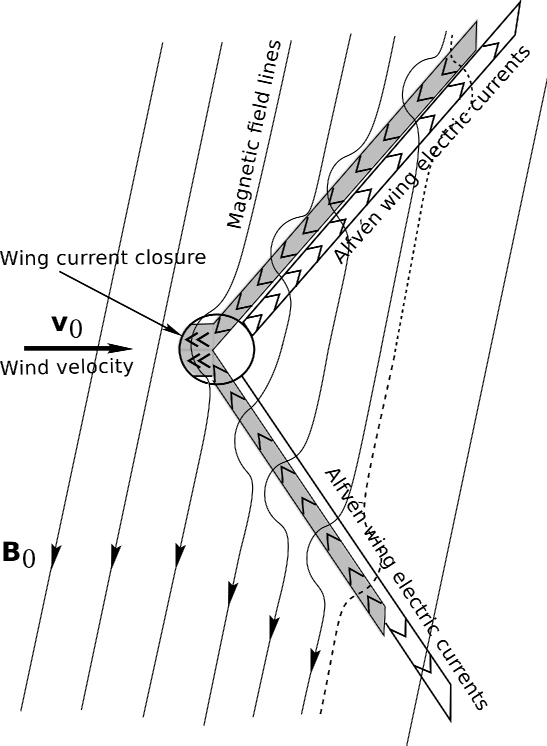
Figure 2: The Alfvénic wake of the planet seen from above the equatorial plane.

a conductance which is associated with the impedance of vacuum, equal to ${\mathcal{R}}_{\infty}\equiv\mu_{0}c=$ 377 Ohm. The two directions of the currents flows correspond to the invariant vectors ${\bf U}_{+}$ and ${\bf U}_{-}$.The geometrical configuration of this solution is shown in Fig. 2.

Now, we can adapt quite directly the conclusions of Neubauer (1980) to the relativistic inductor. This author considers a specific model of the wake-aligned currents in the Alfvén wing, which he assumes to be flowing on the surface of an infinite cylinder tangent to the planet’s surface, with its axis parallel to Alfvénic characteristics. Equation (67) implies that for such currents the divergence of the electric field vanishes except on the cylinder’s surface. The electric potential can then be found by solving Laplace’s equation, assuming the electric field inside the cylinder to be constant, of intensity $E_{i}$. This simple assumption is motivated by the difficulty to solve for the electromagnetic and flow structure in the immediate vicinity of the solid body. The free parameter $E_{i}$ is the electric field along the planet caused by its ionosphere or surface internal resistance. At large distances from the wake, the electric field converges to the convection field ${\mathbf{E}}_{0}$ given by the perfect MHD relation (21) in the unperturbed wind. Once the electric potential is found, the magnetic field and current distribution in the wake can be deduced, using in particular equation (67).

Neubauer gives useful expressions for the total current $I$ flowing along an Alfvén wing and for the Joule dissipation power in the solid body, $\dot{E}_{J}$. Writing $R_{P}$ for the planet’s radius, he gets:

$$I = 4\,(E_{0}-E_{i})\,R_{P}\,\Sigma_{A}=4\,\left(\,\frac{\Omega_{*}\Psi}{r}-E_{i}\,\right)\,R_{P}\,\Sigma_{A},$$ (71)

$$\dot{E}_{J} = 4\pi\,R_{P}^{2}\ E_{i}\,(E_{0}-E_{i})\ \Sigma_{A}.$$ (72)

The Joule dissipation is maximum when $E_{i}=E_{0}/2$. In our estimations, we shall use Neubauer’s values for $I$ and $\dot{E}_{J}$. Up to unimportant numerical factors, the results (71)–(72) are simply obtained by considering the current $I$ to be driven in a resistive load of resistance $\Sigma_{A}^{-1}$ by a generator of electromotive force $U_{0}=2E_{0}R_{P}$ applied on two opposite sides of a planet of internal resistance ${\mathcal{R}}_{P}$. Neubauer’s parameter $E_{i}$ is related to ${\mathcal{R}}_{P}$ by:

$$\frac{E_{i}}{E_{0}}=\frac{{\mathcal{R}}_{P}}{\Sigma_{A}^{-1}+{\mathcal{R}}_{P}}.$$ (73)

It is very difficult to know what the value of ${\mathcal{R}}_{P}$ really is. We therefore regard it, or $E_{i}$, as unspecified parameters. The planet’s electrical resistance depends on its constitution, on the path of electric currents in it and on the existence or absence of some form of ionosphere. The conductivity of terrestrial silicate rock is of order $\sigma_{rock}=10^{-3}$ Mho m^-1 (Cook 1973). If it is assumed that the wake current closes through a layer of thickness $h$ at the surface of the planet, the electrical resistance ${\mathcal{R}}_{P}$ of the latter would be of order $\sigma_{rock}^{-1}/h$, which numerically amounts to ${\mathcal{R}}_{P}\sim(h_{\mathrm{km}})^{-1}$. As soon as $h$ would be larger than a few meters, which for this low conductivity is reached in a very short time, ${\mathcal{R}}_{P}$ would be comparable to or less than ${\mathcal{R}}_{\infty}$, eventhough the rock intrinsically is a poor conductor. A second generation planet, which could be partly metallic, or a partly molten body, could have lower resistances.

Table 1: Input data about the pulsars. Rotation period and pulsation, surface magnetic field, mass (in solar masses), radius, and Goldreich-Julian current. Source : (Taylor et al. 2000) catalog, in the SIMBAD database. For PSR 1257+12, the mass and the radius are infered from general ideas about pulsars. For PSR 1620-26, the mass has been measured, because the pulsar is in a binary system (with a white dwarf companion).

Name	$P$ (s)	$\Omega_{*}$ ($s^{-1}$)	$B_{*}$ (Gauss)	$M_{*}$ ($M_{\odot}$)	$R_{*}$ (km)	$I_{GJ}$ (A)
PSR 1257+12	0.006	1010.	$8.8\times 10^{8}$	1.4	10.	4.9 $\times 10^{12}$
PSR 1620-26	0.011	567	$3.\times 10^{9}$	1.35	10.	5.4 $\times 10^{12}$
PSR 10 ms	0.010	628.	$10^{8}$	1.5	10.	2.2 $\times 10^{11}$
PSR 1 s	1.	6.283	$10^{12}$	1.5	10.	2.2 $\times 10^{11}$

Table 2: Input data concerning the planets : mass, radius, orbital period, semi-major axis, excentricity. Source : $M_{\oplus}$, $P_{orb}$, $a$, $e$ from ”The Extrasolar Planets Encyclopaedia” (http://exoplanet.eu/index.php). The estimate of $R_{P}$ is based on the hypothesis of an average mass density $\rho_{P}=$ 5000 kg.m^-3.

Name	$M_{P}$ ($M_{\oplus}$)	$R_{P}$ ($R_{\oplus}$)	$P_{orb}$ (day)	$a$ (AU)	$e$
PSR 1257+12 a	0.02	0.28	25.	0.19	0
PSR 1257+12 b	4.3	1.68	66.	0.36	0.0186
PSR 1257+12 c	3.9	1.62	98.	0.46	0.0252
PSR 1620-26 a	794	9,5	36367.	23.
PSR 1s b 10,000km	3.5	1.57	30.	0.21	0.
PSR 10ms b 100 km	$2.\times 10^{-6}$	0.016	20.	0.16	0.3
PSR 10ms b 1 km	$2.\times 10^{-12}$	$1.6\times 10^{-4}$	20.	0.16	0.3
PSR 1 s b 100 km	$2.\times 10^{-6}$	0.016	20.	0.16	0.3
PSR 1 s b 1 km	$2.\times 10^{-12}$	$1.6\times 10^{-4}$	20.	0.16	0.3

Table 3: Electric potential drop, total electric current associated to the Alfvén wing. Electrical energy $\dot{E}_{Jmax}$ dissipated in the Alfvén wing.

Name	$U$ (V)	$I_{AW}$ (A)	$\dot{E}_{Jmax}$ (W)
PSR 1257+12 a	1.1 $\times 10^{12}$	3.0 $\times 10^{9}$	2.5$\times 10^{21}$
PSR 1257+12 b	3,5 $\times 10^{12}$	9.4 $\times 10^{9}$	2.5 $\times 10^{22}$
PSR 1257+12 c	2,6 $\times 10^{12}$	7.0 $\times 10^{9}$	1.4 $\times 10^{22}$
PSR 1620-26 a	6,0 $\times 10^{11}$	1.5 $\times 10^{9}$	7 $\times 10^{20}$
PSR 1s b 10,000 km	3.8 $\times 10^{13}$	1.0 $10^{11}$	2. $\times 10^{24}$
PSR 10ms b 100 km	2.4$\times 10^{9}$	6.$\times 10^{6}$	1.2 $\times 10^{16}$
PSR 10ms b 1 km	2.4$\times 10^{7}$	6.$\times 10^{4}$	1.2 $\times 10^{12}$
PSR 1 s b 100 km	2.4 $\times 10^{11}$	6$\times 10^{8}$	1.2 $\times 10^{20}$
PSR 1 s b 1 km	2.4 $\times 10^{9}$	6.$\times 10^{6}$	1.2 $\times 10^{16}$

6 Discussion and conclusion

This work shows that a planet orbiting a pulsar develops a system of Alfvén wings, caused by its interaction with the sub-Alfvénic Poynting-flux-dominated pulsar wind. A system of strong electric currents is set. Although this current cannot reach the inner pulsar’s magnetosphere, it is nevertheless interesting to compare it to the current at the origin of the pulsar’s magnetospheric activity, the Goldreich-Julian current $J_{GJ}$. This latter current results from the electromotive field generated by the fast rotation of the highly magnetized neutron star and its surrounding magnetosphere. For a dipole magnetic field, the Goldreich-Julian current density is

$$J_{GJ}=c\epsilon_{0}\Omega_{*}B_{*},$$ (74)

and the total current is of the order of

$$I_{GJ}\sim\pi R_{PC}^{2}J_{GJ},$$ (75)

where $R_{PC}\sim R_{*}^{3/2}(\Omega_{*}/c)^{1/2}$ is the polar cap radius (Kirk et al. 2009). Various values of the Goldreich-Julian current $I_{GJ}$ are given in Table 1. A look at table 3 allows for comparisons between $I_{AW}$ and $I_{GJ}$. It can be seen that in the case of the four known planets, the electric current in the Alfv n wings is smaller than the Goldreich-Julian current by three orders of magnitude. It is also much smaller in the case of small bodies. But a planet orbiting a ”standard” pulsar with a typical 1 second period and $10^{12}$ G magnetic field would have an Alfv n wing current $I_{AW}$ of similar amplitude as the Goldreich-Julian current $I_{GJ}$. This is not negligible, when we see that $I_{GJ}$ is the basic engine of the pulsar’s electrodynamics.

The practical consequences of such a current are expected to be of two kinds : it is shown in a companion paper (Mottez & Heyvaerts 2011) that it can exert an ortho-radial force upon the planet that can, if the magnetic to mechanical energy coupling is efficient enough, have an incidence on the orbit of small circum-pulsar objects such as asteroids or comets. The second incidence, more relevant to massive objects such as planets, is a possibly associated electromagnetic signature, which might be detectable.

Does the Alfv n wing dominates, in terms of energy, the direct mechanical action exerted by the wind on the companion ? To answer this question, we can compare the flux of magnetic energy, $F_{M}$ with the flux of mechanical energy, $F_{K}$, received the companion by direct impingement. The ratio of the Poynting flux to the mechanical energy flux is

$$\frac{F_{M}}{F_{K}}=\frac{c\ (B_{0\phi}^{2}/\mu_{0})}{c\ (\gamma_{0}\rho_{0}c^{2})}.$$ (76)

Introducing $\sigma_{0}$ and $\Psi$ with the Eqs. (5,6,10), and $v_{0r}\sim c$,

$$\frac{F_{M}}{F_{K}}=\frac{\sigma_{0}}{\gamma_{0}}.$$ (77)

In the case discussed above where $\gamma_{0}\sim\sigma_{0}^{1/3}$, and $\sigma_{0}>>1$,

$$\frac{F_{M}}{F_{K}}\sim\sigma_{0}^{2/3}>>1.$$ (78)

Therefore, we expect that for a Poynting-flux-dominated wind, most of the energy exchange with the pulsar’s companion comes from the magnetic field. The Eq. (72) provides a more precise insight of what is effectively involved into the wind-companion interaction. Considering $E_{i}=E_{0}$ and $E_{0}\sim cB_{\phi}$,

$$\frac{{\dot{E}}_{J}}{\pi R_{P}^{2}}\approx E_{0}^{2}\,\Sigma_{A}\approx\frac{c^{2}B_{\phi}^{2}}{\mu_{0}c}=c\ \frac{B_{\phi}^{2}}{\mu_{0}}.$$ (79)

This amounts to the totality of the Poynting flux intercepted by the pulsar’s companion. It is therefore larger (by a factor $\sigma_{0}^{2/3}$) than the mechanical energy captured by direct impigement.

This paper rests on the fact that the wind velocity $v_{0}$ is slower than the Alfv n wave velocity $V_{A}$. Otherwise, there would be no Alfv n wing. In the case of an ideal MHD radial wind, the Lorentz factor asymptotically approaches $\sigma_{0}^{1/3}$ and Eq. (9) shows that the wind remains sub-Alfv nic at any distance. If however it is formally considered that the asymptotic Lorentz factor $\gamma_{0\infty}$ scales as $\sigma^{a}$ instead, with an exponent $a\neq 1/3$, then if $a>1/3$, $M_{A\infty}=1+\sigma^{a-1}-\sigma^{-2a}\sim 1+\sigma^{a-1}>1$. Therefore, in that case, a transition form a sub-Alfv nic to a super-Alfv nic wind occurs at a finite distance. Observations of the equatorial sectors of winds driving pulsar wind nebulae show lower values of the asymptotic magnetization (Kennel & Coroniti 1984a, b; Gaensler et al. 2002) and various authors suggest that the asymptotic value of the Lorentz factor is rather $\gamma_{\infty}\sim\sigma_{0}$. Arons (2004) argues that dissipation must occur in the asymptotic wind zone, in order to understand the observed high Lorentz factors and the low magnetization. Begelman & Li (1994) show that when the flux tubes diverge faster than radially, the fast magnetosonic point can occur closer to the light cylinder, implying an even closer Alfv nic point. In such a circumstance, the existence of Alfv n wings would depend on the distance from the star to the planet, combined with the effect of a non-radial diverging wind flow, or dissipation.

Let us come back to the hypothesis of a planet in a sub-Alfv nic wind. The present work provides only orders of magnitude estimates for the emitted current. The behaviour of the Alfvén wing at close vicinity of the planet would need a more detailed study. We have considered here, as in many other papers concerning pulsars, the case of a neutron star magnetic field that is aligned with the rotation axis. The study of oblique rotators raises more complicated problems. The pulsar wind may have different properties, and carry, even in the equatorial plane, a non-zero $B^{\theta}$ component that oscillates at the pulsar rotation rate $\Omega_{*}$. An Alfvén wavelength (propagating at $\sim c$) with $P=6$ ms (case of PSR B1257+12) is of the order of 1800 km, which is less than a typical planetary radius. This would put the assumption of stationarity into question, though less severely in the case of a standard pulsar with $P\sim 1$s, where the wavelength (about 300 000 km) would be much larger than the planetary radius.

In spite of the preliminary character of our model, our study shows that the consideration of Alfvén wings associated to planets orbiting pulsars deserve some attention.

The question of the radio emissions possibly associated to the Alfvén wings will be addressed in a forthcoming paper. Such emissions would provide astronomers with observational data relevant to the wind/planet interaction.