A two step, fourth order, nearly-linear method with energy preserving properties

Abstract

We introduce a family of fourth order two-step methods that preserve the energy function of canonical polynomial Hamiltonian systems. Each method in the family may be viewed as a correction of a linear two-step method, where the correction term is $O(h^{5})$ ($h$ is the stepsize of integration). The key tools the new methods are based upon are the line integral associated with a conservative vector field (such as the one defined by a Hamiltonian dynamical system) and its discretization obtained by the aid of a quadrature formula. Energy conservation is equivalent to the requirement that the quadrature is exact, which turns out to be always the case in the event that the Hamiltonian function is a polynomial and the degree of precision of the quadrature formula is high enough. The non-polynomial case is also discussed and a number of test problems are finally presented in order to compare the behavior of the new methods to the theoretical results.

1 Introduction and Background

We consider canonical Hamiltonian systems in the form

$$\frac{dy}{dt}=J\nabla H(y),\qquad J=\left(\begin{array}[]{cc}0&I_{m}\\ -I_{m}&0\end{array}\right),\qquad y(t_{0})=y_{0}\in{\mathbb{R}}^{2m},\vspace{-.5em}$$ (1)

where $H(y)$ is a smooth real-valued function. Our interest is in researching numerical methods that provide approximations $y_{n}\simeq y(t_{0}+nh)$ to the true solution along which the energy is precisely conserved, namely

$$H(y_{n})=H(y_{0}),\qquad\mbox{for all stepsizes }h\leq h_{0}.$$ (2)

The study of energy-preserving methods form a branch of geometrical numerical integration, a research topic whose main aim is preserving qualitative features of simulated differential equations. In this context, symplectic methods have had considerable attention due to their good long-time behavior as compared to standard methods for ODEs [25, 15, 21]. A related interesting approach based upon exponential/trigonometric fitting may be found in [20, 27, 26]. Unfortunately, symplecticity cannot be fully combined with the energy preservation property [16], and this partly explains why the latter has been absent from the scene for a long time.

Among the first examples of energy-preserving methods we mention discrete gradient schemes [17, 23] which are defined by devising discrete analogs of the gradient function. The first formulae in this class had order at most two but recently discrete gradient methods of arbitrarily high order have been researched by considering the simpler case of systems with one-degree of freedom [12, 13].

Here, the key tool we wish to exploit is the well-known line integral associated with conservative vector fields, such us the one defined at (1), as well as its discrete version, the so called discrete line integral. Interestingly, the line integral provides a means to check the energy conservation property, namely

$$\begin{array}[]{rl}H(y(t_{1}))-H(y_{0})&=\displaystyle\int_{y_{0}\rightarrow y(t_{1})}\nabla H(y)\mathrm{d}y=h\int_{0}^{1}y^{\prime}(t_{0}+\tau h)^{T}\nabla H(y(t_{0}+\tau h))\mathrm{d}\tau\\[9.95863pt] &=h\displaystyle\int_{0}^{1}\nabla^{T}H(y(t_{0}+\tau h))J^{T}\nabla H(y(t_{0}+\tau h))\mathrm{d}\tau=0,\end{array}$$

with $h=t_{1}-t_{0}$, that can be easily converted into a discrete analog by considering a quadrature formula in place of the integral.

The discretization process requires to change the curve $y(t)$ in the phase space ${\mathbb{R}}^{2m}$ to a simpler curve $\sigma(t)$ (generally but not necessarily a polynomial), which is meant to yield the approximation at time $t_{1}=t_{0}+h$, that is $y(t_{0}+h)=\sigma(t_{0}+h)+O(h^{p+1})$, where $p$ is the order of the resulting numerical method. In a certain sense, the problem of numerically solving (1) while preserving the Hamiltonian function is translated into a quadrature problem.

For example, consider the segment $\sigma(t_{0}+ch)=(1-c)y_{0}+cy_{1}$, with $c\in[0,1]$, joining $y_{0}$ to an unknown point $y_{1}$ of the phase space. The line integral of $\nabla H(y)$ evaluated along $\sigma$ becomes

$${H(y_{1})-H(y_{0})}=h(y_{1}-y_{0})^{T}\int_{0}^{1}\nabla H((1-c)y_{0}+cy_{1})\,\mathrm{d}c.$$ (3)

Now assume that $H(y)\equiv H(q,p)$ is a polynomial of degree $\nu$ in the generalized coordinates $q$ and in the momenta $p$. The integrand in (3) is a polynomial of degree $\nu-1$ in $c$ and can be exactly solved by any quadrature formula with abscissae $c_{1}<c_{2}<\cdots<c_{k}$ in $[0,1]$ and weights $b_{1},\dots,b_{k}$, having degree of precision $d\geq\nu-1$. We thus obtain

$$H(y_{1})-H(y_{0})=h(y_{1}-y_{0})^{T}{\sum_{i=1}^{k}b_{i}\nabla H((1-c_{i})y_{0}+c_{i}y_{1})}.$$

To get the energy conservation property we impose that $y_{1}-y_{0}$ be orthogonal to the above sum, and in particular we choose (for the sake of generality we use $f(y)$ in place of $J\nabla H(y)$ to mean that the resulting method also makes sense when applied to a general ordinary differential equation $y^{\prime}=f(y)$)

$$y_{1}=\displaystyle y_{0}+h\sum_{i=1}^{k}b_{i}f(Y_{i}),\qquad Y_{i}=(1-c_{i})y_{0}+c_{i}y_{1},\quad i=1,\dots,k.$$ (4)

Formula (4) defines a Runge–Kutta method with Butcher tableau $\begin{array}[]{c|c}c&cb^{T}\\ \hline\cr&b^{T}\end{array}$, where $c$ and $b$ are the vectors of the abscissae and weights, respectively. The stages $Y_{i}$ are called silent stages since their presence does not affect the degree of nonlinearity of the system to be solved at each step of the integration procedure: the only unknown is $y_{1}$ and consequently (4) defines a mono-implicit method. Mono-implicit methods of Runge–Kutta type have been researched in the past by several authors (see, for example, [9, 1, 10, 8] for their use in the solution of initial value problems).

Methods such as (4) date back to 2007 [18, 19] and are called $k$-stage trapezoidal methods since on the one hand the choice $k=2$, $c_{1}=0$, $c_{2}=1$ leads to the trapezoidal method and on the other hand all other methods evidently become the trapezoidal method when applied to linear problems.

Generalizations of (4) to higher orders require the use of a polynomial $\sigma$ of higher degree and are based upon the same reasoning as the one discussed above. Up to now, such extensions have taken the form of Runge–Kutta methods [4, 5, 6]. It has been shown that choosing a proper polynomial $\sigma$ of degree $s$ yields a Runge–Kutta method of order $2s$ with $k\geq s$ stages. The peculiarity of such energy-preserving formulae, called Hamiltonian Boundary Value Methods (HBVMs), is that the associated Butcher matrix has rank $s$ rather than $k$, since $k-s$ stages may be cast as linear combinations of the remaining ones, similarly to the stages $Y_{i}$ in (4). As a consequence, the nonlinear system to be solved at each step has dimension $2ms$ instead of $2mk$, which is better visualized by recasting the method in block-BVM form [4].

In the case where $H(y)$ is not a polynomial, one can still get a practical energy conservation by choosing $k$ large enough so that the quadrature formula approximates the corresponding integral to within machine precision. Strictly speaking, taking the limit as $k\rightarrow\infty$ leads to limit formulae where the integrals come back into play in place of the sums. For example, letting $k\rightarrow\infty$ in (4) just means that the integral in (3) must not be discretized at all, which would yield the Averaged Vector Field method $y_{1}=y_{0}+h\int_{0}^{1}f((1-c)y_{0}+cy_{1})\,\mathrm{d}c$, (see [11, 24] for details).

In this paper we start an investigation that follows a different route. Unlike the case with HBVMs, we want now to take advantage of the previously computed approximations to extend the class (4) in such a way to increase the order of the resulting methods, much as the class of linear multistep method may be viewed as a generalization of (linear) one step methods. The general question we want to address is whether there exist $k$-step mono-implicit energy-preserving methods of order greater than two. Clearly, the main motivation is to reduce the computational cost associated with the implementation of HBVMs.

The purpose of the present paper is to give an affermative answer to this issue in the case $k=2$. More specifically, the method resulting from our analysis, summarized by formula (16), may be thought of as a nearly linear two-step method in that it is the sum of a fourth order linear two-step method, formula (18), plus a nonlinear correction of higher order.

The paper is organized as follows. In Section 2 we introduce the general formulation of the method, by which we mean that the integrals are initially not discretized to maintain the theory at a general level. In this section we also report a brief description of the HBVM of order four, since its properties will be later exploited to deduce the order of the new method: this will be the subject of Section 3. Section 4 is devoted to the discretization of the integrals, which will produce the final form of the methods making them ready for implementation. A few test problems are presented in Section 5 to confirm the theoretical results.

2 Definition of the method

Suppose that $y_{1}$ is an approximation to the true solution $y(t)$ at time $t_{1}=t_{0}+h$, where $h>0$ is the stepsize of integration. More precisely, we assume that

• $y(t_{1})=y_{1}+O(h^{p+1})$ with $p\geq 4$;

• $H(y_{1})=H(y_{0})$, which means that $y_{1}$ lies on the very same manifold $H(y)=H(y_{0})$ as the continuous solution $y(t)$.

The two above assumptions are fulfilled if, for example, we compute $y_{1}$ by means of a HBVM (or an $\infty$-HBVM [5]) of order $p\geq 4$. The new approximation $y_{2}\simeq y(t_{2})\equiv y(t_{0}+2h)$ is constructed as follows.

Consider the quadratic polynomial $\sigma(t_{0}+2\tau h)$ that interpolates the set of data $\{(t_{0}+jh,y_{j})\}_{j=0,1,2}$. Expanded along the Newton basis $\{P_{j}(\tau)\}$ defined on the nodes $\tau_{0}=0$, $\tau_{1}=\frac{1}{2}$, $\tau_{2}=1$, the polynomial $\sigma$ takes the form (for convenience we order the nodes as $\tau_{0},\tau_{2},\tau_{1}$)

$$\sigma(t_{0}+2\tau h)=y_{0}+(y_{2}-y_{0})\tau+2(y_{2}-2y_{1}+y_{0})\tau(\tau-1).$$ (5)

As $\tau$ ranges in the interval $[0,1]$, the $2m$-length vector $\gamma(\tau)\equiv\sigma(t_{0}+2\tau h)$ describes a curve in the phase space ${\mathbb{R}}^{2m}$. The line integral of the conservative vector field $\nabla H(y)$ along the curve $\gamma$ will match the variation of the energy function $H(y)$, that is

$$\begin{array}[]{rl}H(y_{2})-H(y_{0})&=\displaystyle\int_{y_{0}\rightarrow y_{2}}\nabla H(y)\mathrm{d}y=\int_{0}^{1}\left[\gamma^{\prime}(\tau)\right]^{T}\nabla H(\gamma(\tau))\,\mathrm{d}\tau\\[14.22636pt] &\displaystyle=(y_{2}-y_{0})^{T}\int_{0}^{1}\nabla H(\gamma(\tau))\,\mathrm{d}\tau+2(y_{2}-2y_{1}+y_{0})^{T}\int_{0}^{1}(2\tau-1)\nabla H(\gamma(\tau))\,\mathrm{d}\tau.\end{array}$$

The energy conservation condition $H(y_{2})=H(y_{0})$ yields the following equation in the unknown $z\equiv y_{2}$

$$(z-y_{0})^{T}\int_{0}^{1}\nabla H(\gamma(\tau))\,\mathrm{d}\tau=-2(z-2y_{1}+y_{0})^{T}\int_{0}^{1}(2\tau-1)\nabla H(\gamma(\tau))\,\mathrm{d}\tau.$$ (6)

The method we are interested in has the form $y_{2}=\Psi_{h}(y_{0},y_{1})$, where $\Psi_{h}$ is implicitly defined by the following nonlinear equation in the unknown $z$:

$$z=y_{0}+2hJa(z)+\frac{r(z)}{||a(z)||_{2}^{2}}a(z),\qquad\mbox{with}~{}~{}a(z)=\int_{0}^{1}\nabla H(\gamma(\tau))\,\mathrm{d}\tau,$$ (7)

where the residual $r(z)$ is defined as

$$r(z)\equiv-2(z-2y_{1}+y_{0})^{T}\int_{0}^{1}(2\tau-1)\nabla H(\gamma(\tau))\,\mathrm{d}\tau.$$ (8)

A direct computation shows that any solution $z^{\ast}$ of (7) also satisfies (6). In the next section we will show that (7) admits a unique solution $y_{2}\equiv z^{\ast}$ satisfying the order condition $y_{2}=y(t_{0}+2h)+O(h^{5})$. Such a result will be derived by regarding (7) as a perturbation of the HBVM of order $4$ and, in turn, by comparing the two associated numerical solutions. To this end and to better explain the genesis of formula (7) and the role of the integrals therein, a brief introduction of the HBVM formula of order four is in order.

2.1 HBVM of order four

Suppose that both $y_{1}$ and $y_{2}$ are unknown (so now $y_{1}$ is no longer given a priori as indicated by assumption ($A_{1}$)): let us call them $u_{1}$ and $u_{2}$ respectively. For (6) to be satisfied, we can impose the two orthogonality conditions

$$\left\{\begin{array}[]{l}\displaystyle u_{2}-y_{0}=\eta_{1}hJ\int_{0}^{1}\nabla H(\gamma(\tau))\,\mathrm{d}\tau,\\[14.22636pt] \displaystyle u_{2}-2u_{1}+y_{0}=\eta_{2}hJ\int_{0}^{1}(2\tau-1)\nabla H(\gamma(\tau))\,\mathrm{d}\tau,\end{array}\right.$$ (9)

giving rise to a system of two block-equations (the curve $\gamma(\tau)=\sigma(t_{0}+2\tau h)$ is as in (5) with $u_{1}$ and $u_{2}$ in place of $y_{1}$ and $y_{2}$). Setting the free constants $\eta_{1}$ and $\eta_{2}$ equal to $2$ and $3$, respectively, confers the highest possible order, namely $4$, on the resulting method: $u_{2}=y(t_{0}+2h)+O(h^{5})$ (see [19] for details). Furthermore, it may be shown that the internal stage $u_{1}$ satisfies the order condition $u_{1}=y(t_{0}+h)+O(h^{4})$.

Evidently, the implementation of (9) on a computer cannot leave out of consideration the issue of solving the integrals appearing in both equations. Two different situations may emerge:

• the Hamiltonian function $H(y)$ is a polynomial of degree $\nu$. In such a case, the two integrals in (9) are exactly computed by a quadrature formula having degree of precision $d\geq 2\nu-1$.

• $H(y)$ is not a polynomial, nor do the two integrands admit a primitive function in closed form. Again, an appropriate quadrature formula can be used to approximate the two integrals to within machine precision, so that no substantial difference is expected during the implementation process by replacing the integrals by their discrete counterparts.

Case (a) gives rise to an infinite family of Runge-Kutta methods, each depending on the specific choice (number and distribution) of nodes the quadrature formula is based upon (see [5] for a general introduction on HBVMs and [6] for their relation with standard collocation methods). For example, choosing $k$ nodes according to a Gauss distribution over the interval $[0,1]$ results in a method that precisely conserves the energy if applied to polynomial canonical Hamiltonian systems with $\nu\leq k$ and that becomes the classical $2$-stage Gauss collocation method when $k=2$. On the other hand, choosing a Lobatto distribution yields a Runge-Kutta method that preserves polynomial Hamiltonian functions of degree $\nu\leq k-1$ and that becomes the Lobatto IIIA method of order four when $k=2$.

The method resulting from case (b) are undistinguishable from the original formulae (9) in that they are energy-preserving up to machine precision when applied to any regular canonical Hamiltonian system. Stated differently, (9) may be viewed as the limit of the family of HBVMs of order four, as the number of nodes tends to infinity. For this reason the limit formulae (9) have been called $\infty$-HBVM of order $4$ (see [5]).

Remark 1.

In the present context, $y_{1}$ being a known quantity, the unknown $z$ in (6) cannot in general satisfy, at the same time, both orthogonality conditions in (9). However, since $y_{1}$ may be thought of as an approximation of order four to the quantity $u_{1}$ in (9), should we only impose the first orthogonality condition, namely

$$z-y_{0}=2hJa(z),$$ (10)

we would expect the residual $r(z)$ (the right hand side of (6)) to be very small. This suggests that a solution to (6) that yields an approximation of high order to $y(t_{0}+2h)$ may be obtained by allowing a small deviation from orthogonality in (10). This is accomplished by setting $z-y_{0}=2hJa(z)+\delta a(z)$, and by tuning the perturbation parameter $\delta$ in such a way that (6) be satisfied: this evidently gives $\delta=\frac{r(z)}{||a(z)||_{2}^{2}}$ and we arrive at (7).

3 Analysis of the method

Results on the existence and uniqueness of a solution of (7) as well as on its order of accuracy will be derived by first analyzing the simpler nonlinear system

$$z=y_{0}+2hJa(z),\qquad\mbox{with}~{}~{}a(z)=\int_{0}^{1}\nabla H(\gamma(\tau))\,\mathrm{d}\tau,$$ (11)

obtained by neglecting the correction term $\frac{r(z)}{||a(z)||_{2}^{2}}a(z)$. For $z\in{\mathbb{R}}^{2m}$ we set (see (5))

$$\gamma_{z}(\tau)=y_{0}+(z-y_{0})\tau+2(z-2y_{1}+y_{0})\tau(\tau-1),$$ (12)

and (see (11))

$$\Phi(z)=y_{0}+2hJa(z).$$ (13)

In the following $||\cdot||$ will denote the $2$-norm.

Lemma 1.

There exist positive constants $\rho$ and $h_{0}$ such that, for $h\leq h_{0}$, system (11) admits a unique solution $\hat{z}$ in the ball $B(y_{0},\rho)$ of center $y_{0}$ and radius $\rho$.

Proof.

We show that constants $h_{0},\rho>0$ exist such that the function defined in (13) satisfies the following two conditions for $h\leq h_{0}$:

• $\Phi(z)$ is a contraction on $B(y_{0},\rho)$, namely

  $$\forall z,w\in B(y_{0},\rho),\quad||\Phi(z)-\Phi(w)||\leq L||z-w||,\qquad\mbox{with}\quad L<1;$$

• $||\Phi(y_{0})-y_{0}||\leq(1-L)\rho$.

The contraction mapping theorem can then be applied to obtain the assertion.

Let $B(y_{0},\rho)$ a ball centered at $y_{0}$ with radius $\rho$. We can choose $h^{\prime}_{0}$ and $\rho$ small enough that the image set $\Omega=\{\gamma_{z}(\tau):\tau\in[0,1],~{}z\in B(y_{0},\rho),~{}h\leq h^{\prime}_{0}\}$ is entirely contained in a ball $B(y_{0},\rho^{\prime})$ which, in turn, is contained in the domain of $\nabla^{2}H(y)$. We set

$$M_{\rho}=\max_{w\in B(y_{0},\rho^{\prime})}\left\|\nabla^{2}H(w)\right\|.$$

From (11) and (12) we have

$$\frac{\partial a(z)}{\partial z}=\int_{0}^{1}\nabla^{2}H(\gamma_{z}(\tau))\frac{\partial\gamma_{z}}{\partial z}\,\mathrm{d}\tau=\int_{0}^{1}\nabla^{2}H(\gamma_{z}(\tau))\,\tau(2\tau-1)\,\mathrm{d}\tau$$

and hence

$$\left\|\frac{\partial a(z)}{\partial z}\right\|\leq M_{\rho}\int_{0}^{1}\tau|2\tau-1|\,\mathrm{d}\tau=\frac{1}{4}M_{\rho}.$$

Consequently (a) is satisfied by choosing

$$L=\frac{h}{2}M_{\rho}$$ (14)

and $h_{0}<\min\{\frac{2}{M_{\rho}},h^{\prime}_{0}\}$. Concerning (b), we observe that

$$\Phi(y_{0})-y_{0}=2hJa(y_{0})=2hJ\int_{0}^{1}\nabla H(y_{0}+4(y_{0}-y_{1})\tau(\tau-1))\,\mathrm{d}\tau,$$

hence $||\Phi(y_{0})-y_{0}||=2h||a(y_{0})||$ with $||a(y_{0})||$ bounded with respect to $h$. Since $L$ vanishes with $h$ (see (14)), we can always tune $h_{0}$ in such a way that $2h||a(y_{0})||\leq(1-L)\rho$. ∎

Lemma 2.

The solution $\hat{z}$ of (11) satisfies $y(t+2h)-\hat{z}=O(h^{5})$.

Proof.

Under the assumption ($A_{1}$), (11) may be regarded as a perturbation of system (9), since $y_{1}$ and $u_{1}$ are $O(h^{5})$ and $O(h^{4})$ close to $y(t+h)$ respectively. Since $u_{2}=y(t+2h)+O(h^{5})$, we can estimate the accuracy of $\hat{z}$ as an approximation of $y(t+2h)$ by evaluating its distance from $u_{2}$.

Let $\tilde{\gamma}(\tau)$ be the underlying quadratic curve associated with the HBVM defined by (9), namely

$$\tilde{\gamma}(\tau)\equiv y_{0}+(u_{2}-y_{0})\tau+2(u_{2}-2u_{1}+y_{0})\tau(\tau-1).$$ (15)

Considering that (see (12))

$$\gamma_{u_{2}}(\tau)\equiv y_{0}+(u_{2}-y_{0})\tau+2(u_{2}-2y_{1}+y_{0})\tau(\tau-1)=\tilde{\gamma}(\tau)+4(u_{1}-y_{1})\tau(\tau-1),$$

from the first equation in (9) and (13) we get

$$\begin{array}[]{rl}\Phi(u_{2})=&\displaystyle y_{0}+2hJ\int_{0}^{1}\nabla H(\gamma_{u_{2}}(\tau))\,\mathrm{d}\tau=y_{0}+2hJ\int_{0}^{1}\nabla H(\tilde{\gamma}(\tau))\,\mathrm{d}\tau\\[11.38092pt] &\displaystyle+8hJ\int_{0}^{1}\nabla^{2}H(\tilde{\gamma}(\tau))\tau(\tau-1)\,\mathrm{d}\tau\cdot(u_{1}-y_{1})+O(||u_{1}-y_{1}||^{2})\\[11.38092pt] =&\displaystyle u_{2}+O(h^{5}).\end{array}$$

If $h$ is small enough, $u_{2}$ will be inside the ball $B(y_{0},\rho)$ defined in Lemma 1. The Lipschitz condition yields (see (14))

$$||\hat{z}-u_{2}||=||\Phi(\hat{z})-\Phi(u_{2})+O(h^{5})||\leq\frac{h}{2}M_{\rho}||\hat{z}-u_{2}||+O(h^{5}),$$

and hence $||\hat{z}-u_{2}||=O(h^{5})||$. ∎

The above result states that (11) defines a method of order $4$ which is a simplified (non corrected) version of our conservative method defined at (7). In Section 5 the behavior of these two methods will be compared on a set of test problems. We now state the analogous results for system (7).

Theorem 3.

Under the assumption ($A_{1}$), for $h$ small enough, equation (7) admits a unique solution $z^{\ast}$ satisfying $y(t+2h)-z^{\ast}=O(h^{5})$.

Proof.

Consider the solution $\hat{z}$ of system (11). We have (see (15))

$$\gamma_{\hat{z}}(\tau)-\tilde{\gamma}(\tau)=(\hat{z}-u_{2})\tau(2\tau-1)+4(u_{1}-y_{1})\tau(\tau-1)=O(h^{5}),$$

and

$$\hat{z}-2y_{1}+y_{0}=u_{2}-2u_{1}+y_{0}+O(h^{5}).$$

Hence, by virtue of (9),

$$r(\hat{z})=-2\left[(u_{2}-2u_{1}+y_{0})+O(h^{5})\right]^{T}\left[\int_{0}^{1}(2\tau-1)\nabla H(\tilde{\gamma}(\tau))\,\mathrm{d}\tau+O(h^{5})\right]=O(h^{5}).$$

Since $a(\hat{z})$ is bounded with respect to $h$, it follows that, in a neighborhood of $\hat{z}$, system (7) may be regarded as a perturbation of system (11), the perturbation term being $R(z,h)\equiv\frac{r(z)}{||a(z)||_{2}^{2}}a(z)$.

Consider the ball $B(\hat{z},R(\hat{z},h))$: since $\hat{z}=y_{0}+O(h)$, and $R(\hat{z},h)=O(h^{5})$, this ball is contained in $B(y_{0},\rho)$ defined in Lemma 1 and the perturbed function $\Phi(z)+R(z,h)$ is a contraction therein, provided $h$ is small enough. Evaluating the right-hand side of (7) at $z=\hat{z}$ we get

$$y_{0}+2hJa(\hat{z})+R(\hat{z},h)=\hat{z}+R(\hat{z},h),$$

which means that property (b) listed in the proof of Lemma 1, with $\hat{z}$ in place of $y_{0}$, holds true for the perturbed function $y_{0}+2hJa(z)+R(z,h)$, and the contraction mapping theorem may be again exploited to deduce the assertion. ∎

4 Discretization

As was stressed in Section 2, formula (7) is not operative unless a technique to solve the two integrals is taken into account. The most obvious choice is to compute the integrals by means of a suitable quadrature formula which may be assumed exact in the case where the Hamiltonian function is a polynomial, and to provide an approximation to within machine precision in all other cases.

Hereafter we assume that $H(q,p)$ is a polynomial in $q$ and $p$ of degree $\nu$. Since $\gamma(\tau)$ has degree two, it follows that the integrand functions appearing in the definitions of $a(z)$ and $r(z)$ at (7) and (8) have degree $2\nu-2$ and $2\nu-1$ respectively and can be solved by any quadrature formula with abscissae $c_{1}<c_{2}<\cdots<c_{k}$ in $[0,1]$ and weights $b_{1},\dots,b_{k}$, having degree of precision $d\geq 2\nu-1$. In place of (7) we now consider the equivalent form suitable for implementation

$$y_{2}=y_{0}+2hJ\sum_{i=1}^{k}b_{i}\nabla H(\gamma(c_{i}))+G(y_{0},y_{1},y_{2}),$$ (16)

where

$$G(y_{0},y_{1},y_{2})=\frac{-2(y_{2}-2y_{1}+y_{0})^{T}\sum_{i=1}^{k}b_{i}(2c_{i}-1)\nabla H(\gamma(c_{i}))}{\|\sum_{i=1}^{k}b_{i}\nabla H(\gamma(c_{i}))\|_{2}^{2}}\,\sum_{i=1}^{k}b_{i}\nabla H(\gamma(c_{i})).$$

Notice that from (5) we get

$$\gamma(c_{i})=(1-3c_{i}+2c_{i}^{2})y_{0}+4c_{i}(1-c_{i})y_{1}+c_{i}(2c_{i}-1)y_{2},$$ (17)

that is, $\gamma(c_{i})$ is a linear combination, actually a weighted average, of the approximations $y_{0}$, $y_{1}$ and $y_{2}$. Therefore, since $G(y_{0},y_{1},y_{2})=O(h^{5})$ (see Lemma 2 and Theorem 3), we may look at this term as a nonlinear correction of the generalized linear multistep method

$$y_{2}=y_{0}+2hJ\sum_{i=1}^{k}b_{i}\nabla H(\gamma(c_{i})).$$ (18)

Example 1.

If $H(q,p)$ is quadratic, we can choose $k=3$, $c_{1}=0$, $c_{2}=\frac{1}{2}$, $c_{3}=1$, $b_{1}=b_{3}=\frac{1}{6}$ and $b_{2}=\frac{2}{3}$, that is we can use Simpson’s quadrature formula to compute the integrals in (7) and (8). Since, in such a case, $\gamma(c_{i})=y_{i-1}$, method (18) becomes

$$y_{2}=y_{0}+\frac{h}{3}J\left(\nabla H(y_{0})+4\nabla H(y_{1})+\nabla H(y_{2})\right),$$

that is, the standard Milne-Simpson’s method.

In all other cases $\gamma(c_{i})$ will differ in general from $y_{j}$, $j=1,2,3$ and may be regarded as an off-point entry in formula (18). In the sequel we will denote the method defined at (16) by $M_{k}$ and its linear part, defined at (18), by $M^{\prime}_{k}$. Of course, the choice of the abscissae distribution influences the energy preserving properties of the method $M_{k}$, as is indicated in Table 1.

Abscissae distribution:	uniform	Lobatto	Gauss
Energy preserving when:	$\deg H\leq\lceil\frac{k}{2}\rceil$	$\deg H\leq k-1$	$\deg H\leq k$

Table 1: Energy preserving properties of method $M_{k}$ for some well-known distributions of the nodes $\{c_{i}\}$.

5 Numerical tests

Hereafter we implement the order four method $M_{k}$ on a few Hamiltonian problems to show that the numerical results are consistent with the theory presented in Section 3. In particular, in the first two problems the Hamiltonian function is a polynomial of degree three and six respectively, while the last numerical test reports the behavior of the method on a non-polynomial problem.

Each step of the integration procedure requires the solution of a nonlinear system, in the unknown $y_{2}$, represented by (16) for the method $M_{k}$ and (18) for the method $M^{\prime}_{k}$. The easiest way (although not the most efficient one) to find out a solution is by means of fixed point iteration that, in the case of the method $M_{k}$, reads

$$z_{s+1}=y_{0}+2hJ\sum_{i=1}^{k}b_{i}\nabla H(\gamma_{z_{s}}(c_{i}))+G(y_{0},y_{1},z_{s}),\qquad s=1,2,\dots,$$ (19)

where $\gamma_{z}$ is defined at (12) and $z_{0}$ is an initial approximation of $y_{2}$ which is then refined by setting $y_{2}=z_{\bar{s}}$ with $z_{\bar{s}}\simeq\lim_{s\rightarrow\infty}z_{s}$. From Theorem 3 and the preceding lemmas we deduce that such a limit always exists provided that $h$ is small enough. The value of $z_{0}$ could be retrieved via an extrapolation based on the previous computed points or by considering the method $M^{\prime}_{k}$ as a predictor for $M_{k}$.

We will consider a Lobatto distribution with an odd number $k$ of abscissae $\{c_{i}\}$. In fact, if $k$ is odd, since $y_{0}=\gamma(0)=\gamma(c_{1})$ and $y_{1}=\gamma(\frac{1}{2})=\gamma(c_{\lceil\frac{k}{2}\rceil})$, we save two function evaluations during the iteration (19).

5.1 Test problem 1

The Hamiltonian function

$$H(q,p)=\frac{1}{2}p^{2}+\frac{1}{2}q^{2}-\frac{1}{6}q^{3}$$ (20)

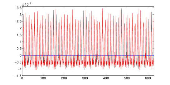
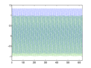
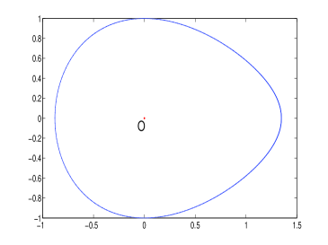
defines the cubic pendulum equation. We can solve it by using five Lobatto nodes to discretize the integrals in (7), thus getting the method $M_{5}$. The corresponding numerical solution, denoted by $(q_{n},p_{n})$, is plotted in Figure 1. For comparison purposes we also compute the numerical solution $(q^{\prime}_{n},p^{\prime}_{n})$ provided by the fourth order method, say $M^{\prime}_{5}$, obtained by neglecting in (7) the correction term, that is by posing $r(z)\equiv 0$. Figure 2 clearly shows the energy conservation property, while Table 2 summarizes the convergence properties of the two methods.

Fig. 1: Numerical solution $(q_{n},p_{n})$ versus time $t_{n}$ (left picture) and on the phase plane (right picture). Parameters: initial condition $y_{0}=[0,\,1]$; stepsize $h=0.5$; integration interval $[0,200\pi]$.

Fig. 2: Hamiltonian function evaluated along the numerical solution $(p_{n},q_{n})$ (horizontal line) and along the numerical solution $(p^{\prime}_{n},q^{\prime}_{n})$ (irregularly oscillating line).

	method $M_{5}$			method $M^{\prime}_{5}$
$h$	error	order	$\max|H(y_{n})-H(y_{0})|$	error	order	$\max|H(y^{\prime}_{n})-H(y_{0})|$
$1$	$3.1\cdot 10^{-2}$		$2.5\cdot 10^{-15}$	$1.1\cdot 10^{-1}$		$1.1008\cdot 10^{-1}$
$2^{-1}$	$3.8\cdot 10^{-4}$	$6.373$	$1.9\cdot 10^{-15}$	$3.1\cdot 10^{-3}$	$5.183$	$2.9680\cdot 10^{-3}$
$2^{-2}$	$2.6\cdot 10^{-5}$	$3.866$	$1.5\cdot 10^{-15}$	$2.5\cdot 10^{-4}$	$3.655$	$1.5755\cdot 10^{-4}$
$2^{-3}$	$1.6\cdot 10^{-6}$	$4.059$	$8.8\cdot 10^{-16}$	$1.8\cdot 10^{-5}$	$3.811$	$8.5163\cdot 10^{-6}$
$2^{-4}$	$9.5\cdot 10^{-8}$	$4.032$	$9.9\cdot 10^{-16}$	$1.2\cdot 10^{-6}$	$3.905$	$4.8883\cdot 10^{-7}$
$2^{-5}$	$5.9\cdot 10^{-9}$	$4.017$	$1.1\cdot 10^{-15}$	$7.6\cdot 10^{-8}$	$3.952$	$2.9131\cdot 10^{-8}$
$2^{-6}$	$3.6\cdot 10^{-10}$	$4.008$	$1.1\cdot 10^{-15}$	$4.9\cdot 10^{-9}$	$3.976$	$1.7771\cdot 10^{-9}$
$2^{-7}$	$2.3\cdot 10^{-11}$	$4.004$	$2.3\cdot 10^{-15}$	$3.1\cdot 10^{-10}$	$3.988$	$1.0968\cdot 10^{-10}$
$2^{-8}$	$1.4\cdot 10^{-12}$	$4.006$	$2.4\cdot 10^{-15}$	$1.9\cdot 10^{-11}$	$3.994$	$6.8121\cdot 10^{-12}$

Table 2: Methods $M_{5}$ (with correction term) and $M^{\prime}_{5}$ (without correction term) are implemented on the cubic pendulum equation (20) on the time interval $[0,10]$ for several values of the stepsize $h$. The order of convergence is numerically evaluated by means of the formula $\log_{2}\frac{\mbox{\rm error}(\frac{h}{2})}{\mbox{\rm error}(h)}$. As was expected, the maximum displacement of the numerical Hamiltonian $H(y_{n})$ from the theoretical value $H(y_{0})$ is close to the machine precision for the method $M_{5}$, independently of the stepsize $h$ used.

5.2 Test problem 2

The Hamiltonian function

$$H(p,q)=\frac{1}{3}p^{3}-\frac{1}{2}p+\frac{1}{30}q^{6}+\frac{1}{4}q^{4}-\frac{1}{3}q^{3}+\frac{1}{6}$$ (21)

has been proposed in [14] to show that symmetric methods may suffer from the energy drift phenomenon even when applied to reversible systems, that is when $H(-p,q)=H(p,q)$. For our experiment, we will use $y_{0}=[0.2,\,0.5]$ as initial condition.

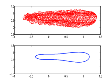
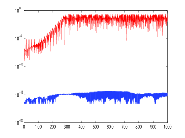
Since $\deg(H(q,p))=6$, we need a Lobatto quadrature based on at least seven nodes to assure that the integrals in (7) are computed exactly. Therefore we solve (21) by method $M_{7}$. For comparison purposes, it is also interesting to show the dynamics of the symmetric non-conservative method $M^{\prime}_{7}$. Figure 3 displays the results obtained by the two methods implemented with stepsize $h=\frac{1}{10}$ over the interval $[0,\,10^{3}]$. In particular, the numerical trajectories generated by method $M^{\prime}_{7}$ and $M_{7}$, are reported in the left-top and left-bottom pictures respectively, while the right picture reports the corresponding error in the Hamiltonian function evaluated along the two numerical solutions, namely $|H(y_{n})-H(y_{0})|$.

Evidently, the numerical solution produced by $M^{\prime}_{7}$ rapidly departs from the level curve $H(q,p)=H(q_{0},p_{0})$ but it remain eventually bounded and the points $(q_{n},p_{n})$ seem to densely fill a bounded region of the phase plane.

On the contrary, since the degree of freedom of the present problem is one, the points $(q_{n},p_{n})$ produced by $M_{7}$ lie on the very same continuous trajectory covered by $y(t)$: this is also confirmed by looking at the bottom graph in the right picture.

Table 3 shows the behavior of method $M_{7}$ applied to problem (21) as the stepsizes $h$ goes to zero. Notice the $O(h^{5})$ rate of convergence to zero for the residual function $r(z)$ in (8).

Fig. 3: Left pictures: numerical solutions in the phase plane computed by method $M^{\prime}_{7}$ (top picture) and $M_{7}$ (bottom picture). Right picture: error in the numerical Hamiltonian function $|H(y_{n})-H(y_{0})|$ produced by the two methods. Parameters: initial condition $y_{0}=[0.2,\,0.5]$; stepsize $h=0.1$; integration interval $[0,1000]$.

	method $M_{7}$
$h$	error	order	$|H(y_{N})-H(y_{0})|$	residual $r(y_{N})$	order of $r(y_{N})$
$2^{-1}$	$4.47\cdot 10^{-2}$		$1.6\cdot 10^{-16}$	$-1.21\cdot 10^{-03}$
$2^{-2}$	$7.38\cdot 10^{-4}$	$5.920$	$4.4\cdot 10^{-16}$	$-3.23\cdot 10^{-06}$	$8.559$
$2^{-3}$	$3.90\cdot 10^{-5}$	$4.243$	$5.8\cdot 10^{-16}$	$-2.15\cdot 10^{-08}$	$7.225$
$2^{-4}$	$2.39\cdot 10^{-6}$	$4.027$	$2.4\cdot 10^{-16}$	$-6.61\cdot 10^{-10}$	$5.029$
$2^{-5}$	$1.49\cdot 10^{-7}$	$4.007$	$2.5\cdot 10^{-15}$	$-2.03\cdot 10^{-11}$	$5.021$
$2^{-6}$	$9.27\cdot 10^{-9}$	$4.002$	$3.2\cdot 10^{-15}$	$-6.27\cdot 10^{-13}$	$5.018$
$2^{-7}$	$5.77\cdot 10^{-10}$	$4.006$	$5.5\cdot 10^{-16}$	$-2.00\cdot 10^{-14}$	$4.972$
$2^{-8}$	$3.16\cdot 10^{-11}$	$4.188$	$5.4\cdot 10^{-15}$	$-5.36\cdot 10^{-16}$	$5.219$

Table 3: Performance of method $M_{7}$ applied to problem (21), with initial condition $y_{0}=[0.2,\,0.5]$, on the time interval $[0,250]$ for several values of the stepsize $h$, as specified in the first column. The second and third columns report the relative error in the last computed point $y_{N}$, $N=T/h$ and the corresponding order of convergence. Since the integrals appearing in (7) are precisely computed by the Lobatto quadrature formula with seven nodes, the error in the numerical Hamiltonian $H(y_{N})$ is zero up to machine precision. The last two columns list the residual $r(y_{N})$ defined in (8) and its order of convergence to zero.

5.3 Test problem 3

We finally consider the non-polynomial Hamiltonian function

$$H(q_{1},q_{2},p_{1},p_{2})=\frac{1}{2}(p_{1}^{2}+p_{2}^{2})-\frac{1}{\sqrt{q_{1}^{2}+q_{2}^{2}}}$$ (22)

that defines the well known Kepler problem, namely the motion of two masses under the action of their mutual gravitational attraction. Taking as initial condition

$$(q_{1}(0),q_{2}(0),p_{1}(0),p_{2}(0))=\left(\begin{array}[]{cccc}1-e,&0,&0,&\sqrt{\frac{1+e}{1-e}}\end{array}\right)^{T}$$ (23)

yields an elliptic periodic orbit of period $2\pi$ and eccentricity $e\in[0,1)$. We have chosen $e=0.6$. Though the vector field fails to be a polynomial in $q_{1}$ and $q_{2}$, we can plan to use a sufficiently large number of quadrature nodes to discretize the integrals in (7) so that the corresponding accuracy is within the machine precision. Under this assumption, and taking aside the effect of the floating point arithmetic, the computer will make no difference between the conservative formulae (7) and their discrete counterparts.

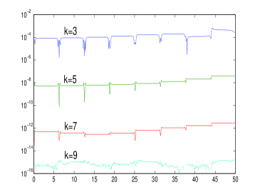
The left picture in Figure 4 explains the above argument. It reports the error $|H(y_{n})-H(y_{0})|$ in the Hamiltonian function for various choices of the number of Lobatto nodes, and precisely $k=3,\,5,\,7,\,9$. We see that the error decreases quickly as the number of nodes is incremented and for $k=9$ it is within the epsilon machine.

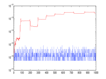
The use of finite arithmetic may sometimes cause a mild numerical drift of the energy over long times, like the one shown in the upper line in the right picture of Figure 4. This is due to the fact that on a computer the numerical solution satisfy the conservation relation $H(y_{n})=H(y_{0})$ up to machine precision times the conditioning number of the nonlinear system that is to be solved at each step.

To prevent the accumulation of roundoff errors we may apply a simple and costless correction technique on the approximation $y_{n}$ which consists in a single step of a gradient descent method (see also [2]). More precisely, the corrected solution $y^{*}_{n}$ is defined by

$$y^{*}_{n}=y_{n}-\alpha\frac{\nabla H(y_{n})}{||\nabla H(y_{n})||_{2}},\qquad\mbox{with}~{}\alpha=\frac{H(y_{n})-H(y_{0})}{||\nabla H(y_{n})||_{2}},$$ (24)

which stems from choosing as $\alpha$ the value that minimizes the linear part of the function $F(\alpha)=H(y_{n}-\alpha\frac{\nabla H(y_{n})}{||\nabla H(y_{n})||_{2}})-H(y_{0})$. The bottom line in the right picture of Figure 4 shows the energy conservation property of the corrected solution.

Fig. 4: Left picture. Error in the numerical Hamiltonian function $|H(y_{n})-H(y_{0})|$ produced by methods $M_{k}$, with $k=3,\,5,\,7,\,9$. Parameters: stepsize $h=0.05$, integration interval $[0,50]$. Right picture. Roundoff errors may cause a drift of the numerical Hamiltonian function (upper line) which can be easily taken under control by coupling the method with a costless correction procedure like the one described at (24).

6 Conclusions

We have derived a family of mono-implicit methods of order four with energy-preserving properties. Each element in the family originates from a limit formula and is defined by discretizing the integral therein by means of a suitable quadrature scheme. This process assures an exact energy conservation in the case where the Hamiltonian function is a polynomial, or a conservation to within machine precision in all other cases, as is also illustrated in the numerical tests. Interestingly, each method may be conceived as a $O(h^{5})$ perturbation of a two-step linear method.

References

• [1] W.M.G. van Bokhoven, Efficient higher order implicit one-step methods for integration of stiff differential equations, BIT 20, 1 (1980), 34–43.
• [2] L. Brugnano, F. Iavernaro, T. Susca, Hamiltonian BVMs (HBVMs): implementation details and applications, AIP Conf. Proc. 1168 (2009), 723–726.
• [3] L. Brugnano, F. Iavernaro and D. Trigiante, The Hamiltonian BVMs (HBVMs) Homepage, arXiv:1002.2757 (URL: http://www.math.unifi.it/~brugnano/HBVM/).
• [4] L. Brugnano, F. Iavernaro and D. Trigiante, Analisys of Hamiltonian Boundary Value Methods (HBVMs): a class of energy-preserving Runge-Kutta methods for the numerical solution of polynomial Hamiltonian dynamical systems, (2009) (submitted) (arXiv:0909.5659).
• [5] L. Brugnano, F. Iavernaro and D. Trigiante, Hamiltonian Boundary Value Methods (Energy Preserving Discrete Line Integral Methods), Jour. of Numer. Anal. Industr. and Appl. Math. 5, 1–2 (2010), 17–37 (arXiv:0910.3621).
• [6] L. Brugnano, F. Iavernaro, D. Trigiante, The Lack of Continuity and the Role of Infinite and Infnitesimal in Numerical Methods for ODEs: the Case of Symplecticity, Applied Mathematics and Computation (to appear), DOI:10.1016/j.amc.2011.03.022, (arXiv:1010.4538).
• [7] L. Brugnano and D. Trigiante, Energy drift in the numerical integration of Hamiltonian problems, Jour. of Numer. Anal. Industr. and Appl. Math. 4, 3–4 (2009), 153-170.
• [8] K. Burrage, F.H. Chipman and P.H. Muir, Order results for mono-implicit Runge–Kutta methods SIAM J. Numer. Anal. 31, 3 (1994), 876–891.
• [9] J.R. Cash, A Class of Implicit Runge–Kutta Methods for the Numerical Integration of Stiff Ordinary Differential Equations, J. ACM 22, 4 (1975), 504–511.
• [10] J.R. Cash and A. Singhal, Mono-implicit Runge–Kutta formulae for the numerical integration of stiff differential systems, IMA J. Numer. Anal. 2, 2 (1982), 211–227.
• [11] E. Celledoni, R.I. McLachlan, D. McLaren, B. Owren, G.R.W. Quispel and W.M. Wright, Energy preserving Runge-Kutta methods, M2AN 43 (2009), 645–649.
• [12] J.L. Cieśliński and B. Ratkiewicz, Improving the accuracy of the discrete gradient method in the one-dimensional case, Phys. Rev. E 81 (2010) 016704.
• [13] J.L. Cieśliński and B. Ratkiewicz, Energy-preserving numerical schemes of high accuracy for one-dimensional Hamiltonian systems, (arXiv:1009.2738).
• [14] E. Faou, E. Hairer and T.-L. Pham, Energy conservation with non-symplectic methods: examples and counter-examples, BIT Numerical Mathematics 44 (2004), 699–709.
• [15] K. Feng, On difference schemes and symplectic geometry. Proceedings of the 5-th Intern, Symposium on differential geometry & differential equations, August 1984, Beijing (1985) 42–58.
• [16] Z. Ge and J.E. Marsden, Lie-Poisson Hamilton-Jacobi theory and Lie-Poisson integrators, Phys. Lett. A, 133 (1988), 134–139.
• [17] O. Gonzales, Time integration and discrete Hamiltonian systems, J. Nonlinear Sci. 6 (1996), 449–467.
• [18] F. Iavernaro and B. Pace, s𝑠s-Stage Trapezoidal Methods for the Conservation of Hamiltonian Functions of Polynomial Type, AIP Conf. Proc. 936 (2007), 603–606.
• [19] F. Iavernaro and D. Trigiante, High-order symmetric schemes for the energy conservation of polynomial Hamiltonian problems, J.Numer. Anal. Ind. Appl. Math. 4, 1-2 (2009), 87–101.
• [20] L.Gr. Ixaru and G. Vanden Berghe, Exponential fitting, Kluwer, Dordrecht 2004.
• [21] B. Leimkuhler and S. Reich, Simulating Hamiltonian Dynamics, Cambridge University Press, Cambridge, 2004.
• [22] R. I. McLachlan and M. Perlmutter, Energy drift in reversible time integration, J. Phys. A 37, 45 (2004), 593–598.
• [23] R.I. McLachlan, G.R.W. Quispel and N. Robidoux, Geometric integration using discrete gradients, R. Soc. Lond. Philos. Trans. Ser. A Math. Phys. Eng. Sci. 357, (1999), 1021–1045.
• [24] G.R.W. Quispel and D.I. McLaren, A new class of energy-preserving numerical integration methods, J. Phys. A 41 (045206), 2008.
• [25] R.D. Ruth, A canonical integration technique, IEEE Trans. Nuclear Science 30,4 (1983) 2669–2671.
• [26] T.E. Simos, High-order closed Newton-Cotes trigonometrically-fitted formulae for long-time integration of orbital problems, Comput. Phys. Comm. 178 (2008), 199–207.
• [27] G. Vanden Berghe and M. Van Daele: Exponentially-fitted Störmer/Verlet methods, J. Numer. Anal. Ind. Appl. Math. 1 (2006), 237–251.