Alternative numerical computation of one-sided Lévy and Mittag-Leffler distributions

Abstract

We consider here the recently proposed closed form formula in terms of the Meijer G-functions for the probability density functions $g_{\alpha}(x)$ of one-sided Lévy stable distributions with rational index $\alpha=l/k$, with $0<\alpha<1$. Since one-sided Lévy and Mittag-Leffler distributions are known to be related, this formula could also be useful for calculating the probability density functions $\rho_{\alpha}(x)$ of the latter. We show, however, that the formula is computationally inviable for fractions with large denominators, being unpractical even for some modest values of $l$ and $k$. We present a fast and accurate numerical scheme, based on an early integral representation due to Mikusinski, for the evaluation of $g_{\alpha}(x)$ and $\rho_{\alpha}(x)$, their cumulative distribution function and their derivatives for any real index $\alpha\in(0,1)$. As an application, we explore some properties of these probability density functions. In particular, we determine the location and value of their maxima as functions of the index $\alpha$. We show that $\alpha\approx 0.567$ and $\alpha\approx 0.605$ correspond, respectively, to the one-sided Lévy and Mittag-Leffler distributions with shortest maxima. We close by discussing how our results can elucidate some recently described dynamical behavior of intermittent systems.

I Introduction

One-sided Lévy stable distributions Levy1 ; Levy2 are ubiquitous in many modern research areas where quantitative and statistical analysis play a major role. (For recent reviews, see, besides Levy2 , the references of PG .) The probability density function of one-sided Lévy distribution of index $\alpha$, $g_{\alpha}(x)$, can be defined by means of its Laplace transform as Levy1

$$\int_{0}^{\infty}e^{-sx}g_{\alpha}(x)\,dx=\exp\left(-s^{\alpha}\right),$$ (1)

for $s\geq 0$, with $0<\alpha<1$. Unfortunately, in spite of its broad applicability, exact solutions of Eq. (1) are available only for a few particular values of $\alpha$. (See, for instance, the Appendix A of Barkai . We notice also that there are some available Mathematica Math and Matlab Matlab packages for the numerical evaluation of $g_{\alpha}(x)$.) In this context, the recent work of Penson and Górska PG is certainly interesting and relevant since they describe a formal solution of Eq. (1) for any rational $\alpha$. In fact, they show that a formula presented without proof in a table of inverse Laplace transforms table could be used to write

$$g_{l/k}(x)=\frac{\sqrt{kl}}{(2\pi)^{(k-l)/2}}\frac{1}{x}G_{l,k}^{k,0}\left(\frac{l^{l}}{k^{k}x^{l}}\left|\begin{array}[]{c}\Delta(l,0)\\ \Delta(k,0)\end{array}\right.\right),$$ (2)

where $G_{p,q}^{m,n}\left(z\left|{}^{(a_{p})}_{(b_{q})}\right.\right)$ is the Meijer G-function math and $\Delta(k,a)$ is the list of $k$ elements given by

$$\Delta(k,a)=\frac{a}{k},\frac{a+1}{k},\cdots,\frac{a+k-1}{k}.$$ (3)

We consider the formula (2) an important advance. Since the Meijer G-function is available in several computer algebra systems, the function $g_{l/k}(x)$ could in principle be evaluated with little programming effort. We notice that the restriction to rational values of $\alpha$ in Eq. (2) does not represent any real problem here. As we will see below, the function $g_{\alpha}(x)$ is continuous in $\alpha$ and, hence, one might compute from Eq. (2) a rational $\alpha$ approximation for $g_{\alpha}(x)$ with any prescribed accuracy. Penson and Górska PG use Eq. (2) to derive other series expression for $g_{l/k}(x)$ and to infer some of its properties. Certainly, the mathematical literature about the Meijer G-function (see, for instance, math and the references therein) will be extremely valuable for the derivation of many other properties of $g_{l/k}(x)$ defined by Eq. (2).

Furthermore, since one-sided Lévy and Mittag-Leffler distributions are known to be related Feller , the formula (2) is also relevant for calculating the probability density functions $\rho^{(r)}_{\alpha}(x)$ of Mittag-Leffler distributions with rational index $\alpha$. We recall that $\rho^{(r)}_{\alpha}(x)$ is also defined from its Laplace transform as well,

$$\int_{0}^{\infty}e^{-sx}\rho^{(r)}_{\alpha}(x)\,dx=\sum_{n=0}^{\infty}\frac{(-sr^{\alpha})^{n}}{\Gamma(1+n\alpha)},$$ (4)

for $s\geq 0$, with $0<\alpha<1$. The right-handed side of Eq. (4) is a particular case of the so-called Mittag-Leffler function math , which reduces to the usual exponential for $\alpha=1$. The free parameter $r$ can be fixed, for instance, by demanding a given first moment for $\rho^{(r)}_{\alpha}(x)$. In particular, since we have from Eq. (4) that

$$\rho^{(r)}_{\alpha}(qx)=q^{-1}\rho^{(r/q^{1/\alpha})}_{\alpha}(x),$$ (5)

for any $q>0$, one can assume $r=1$ without loss of generality. In this case, the superscript is simply dropped. The respective cumulative distribution functions associated to $\rho_{\alpha}(x)$ and $g_{\alpha}(x)$ are known to be related by Feller

$$\Theta_{\alpha}(x)=1-\Lambda_{\alpha}\left({x^{-1/\alpha}}\right),$$ (6)

which leads to

$$\rho_{\alpha}(x)=\frac{1}{\alpha}x^{-(1+1/\alpha)}g_{\alpha}\left({x^{-1/\alpha}}\right).$$ (7)

The relation (7) allows the computation of $\rho_{\alpha}(x)$ by means of the Meijer G-function for rational $\alpha$, thanks to the Penson and Górska formula (2). This is a considerable advance since, as in the previous case, no closed form solution of Eq. (4) is known.

However, the condensed and apparently simple form of Eq. (2) hides a practical pitfall. The evaluation of Eq. (2) is computationally viable only for modest values of $k$ and $l$. For instance, by using the Maple procedure provided by Penson and Górska procedure , we can plot the graphics of $g_{2/3}(x)$ for $x\in[0,2]$ instantaneously in an Intel Core i7 computer running Maple version 14. In order to generate the same graphics with, for instance, $l/k=20/31$, some CPU minutes are necessary. For $l/k=200/301$, we need almost a half an hour to evaluate a single value of $g_{l/k}(x)$! We could not evaluate Eq. (2) for $l/k=2000/3001$ in any reasonable amount of time. Mathematica presents a similar performance. These restrictions, obviously, jeopardize the practical utility of expression (2) since one cannot calculate in reasonable time good approximations to the one-sided Lévy distribution for any $\alpha$. One can understand the rapidity with the evaluation of Eq. (2) becomes unpractical when the values of $l$ and $k$ increase by recalling the definition of the Meijer G-function math

$$G_{p,q}^{m,n}\left(z\left|{}^{(a_{p})}_{(b_{q})}\right.\right)=$$ (8)

$$\frac{1}{2\pi i}\int_{L}\frac{\prod_{j=1}^{m}\Gamma(b_{j}-s)\prod_{j=1}^{n}\Gamma(1-a_{j}+s)}{\prod_{j=m+1}^{q}\Gamma(1-b_{j}+s)\prod_{j=n+1}^{p}\Gamma(a_{j}-s)}z^{s}ds,$$

where $L$ is a carefully chosen integration path on the complex plane. It is possible also to write the Meijer G-function as a sum of $m$ terms involving $\Gamma$ function products as those ones of the integrand in Eq. (8) and the generalized hypergeometric functions ${}_{p}F_{q-1}$ math . As one can see, when asking Maple to evaluate Eq. (2) for $l/k=2000/3001$, one is basically demanding the evaluation of an integral with more than five thousands $\Gamma$ function terms in the integrand, or an intricate combination of more than three thousands generalized hypergeometric functions! Hence, it is not a surprise to have a considerable performance degradation for large values of $l$ and $k$. Another problem with the Maple procedure based in Eq. (2) is that it does not deal efficiently with reducible fractions. For instance, Maple is not able to reduce $g_{5/10}(x)$ to $g_{1/2}(x)$. Moreover, the numerical evaluation of the former is much more time and memory consuming than the latter.

The purpose of the present work is to show that one can compute numerically, in an effective and efficient way, the probability density functions $g_{\alpha}(x)$ and $\rho_{\alpha}(x)$ with arbitrary real index $\alpha\in(0,1)$. Our start point is the Mikusinski’s integral representation for $g_{\alpha}(x)$ Mikusinski

$$g_{\alpha}(x)=\frac{\alpha}{1-\alpha}\frac{1}{\pi x}\int_{0}^{\pi}ue^{-u}\,d\varphi,$$ (9)

with $0<\alpha<1$, where

$$u=\frac{\sin(1-\alpha)\varphi}{\sin\varphi}\left(\frac{\sin\alpha\varphi}{x\sin\varphi}\right)^{\alpha/(1-\alpha)}.$$ (10)

The integral representation (9) has already proven its relevance. In fact, Mikusinski used it to derive more than 40 years ago the some very useful asymptotic expressions for $g_{\alpha}(x)$, namely

$$g_{\alpha}(x)\approx K\frac{\exp{\left(-Ax^{-\alpha/(1-\alpha)}\right)}}{x^{(2-\alpha)/(2-2\alpha)}},$$ (11)

valid for $x\to 0^{+}$ and

$$g_{\alpha}(x)\approx Mx^{-(1+\alpha)},$$ (12)

valid for $x\to\infty$, where

$$A = (1-\alpha)\alpha^{\alpha/(1-\alpha)},$$ (13)

$$K = \frac{\alpha^{1/(2-2\alpha)}}{\sqrt{2\pi(1-\alpha)}},$$ (14)

$$M = \frac{\sin\alpha\pi}{\pi}\Gamma(1+\alpha).$$ (15)

It is easy to check from Eq. (9) that $g_{\alpha}(x)$ is non-negative and smooth in $\alpha\in(0,1)$. Due to Eq. (7), and one has the following asymptotic behavior for $\rho_{\alpha}(x)$

$$\rho_{\alpha}(x)\to\frac{\sin\alpha\pi}{\alpha\pi}\Gamma(1+\alpha),$$ (16)

for $x\to 0^{+}$ and

$$\rho_{\alpha}(x)\approx\frac{K}{\alpha}{x^{(2\alpha-1)/(2-2\alpha)}}{\exp{\left(-Ax^{1/(1-\alpha)}\right)}},$$ (17)

valid for $x\to\infty$. In the next section, we show how to use Eq. (9) to evaluate numerically one-sided Lévy and Mittag-Leffler probability densities, their cumulative distribution function, and their derivatives in a very efficient and reliable way.

We notice that one-sided Lévy stable distributions can be alternatively expressed by means of Fox H-functions WGMN , which are a further generalization of the Meijer G-functions (8), and also by means of Wright functions Mainardi . Unfortunately, the current knowledge about the analytical structure of these functions is still little developed. We wish also to stress here that the numerical computation of stable distributions is not a new problem and several algorithms are already available in the literature and even commercially. In particular, Nolan JPN proposed a robust algorithm based on the integration of the so-called Zolotarev’s (M) representation for stable distributions, which is the base of Mathematica Math and Matlab Matlab packages. An updated reference list on the subject can be found in Ref . However, as we will see, Mikusinski’s representation (9) allows the numerical evaluation of one-sided Lévy stable and Mittag-Leffler distributions with little programming and computational efforts and with the same accuracy of these specialized packages. Furthermore, from the Mikusinski’s representation one will be able to derive some asymptotic expressions with special relevance to physical applications.

II The algorithm

The Mikusinski’s integral representation (9) involves a simple proper integral of a smooth function on the interval $\varphi\in[0,\pi]$. Furthermore, it is easy to obtain from Eq. (9) some analogous formulas for the derivatives of $g_{\alpha}(x)$ and its cumulative distribution function $\Lambda_{\alpha}(x)$. In particular, we have

$$\Lambda_{\alpha}(x) = \frac{1}{\pi}\int_{0}^{\pi}e^{-u}\,d\varphi,$$ (18)

$$g^{\prime}_{\alpha}(x) = \left(\frac{\alpha}{1-\alpha}\right)^{2}\frac{1}{\pi x^{2}}\int_{0}^{\pi}u^{2}e^{-u}\,d\varphi-\frac{1}{1-\alpha}\frac{g_{\alpha}(x)}{x},$$

and

$$g^{\prime\prime}_{\alpha}(x) = \left(\frac{\alpha}{1-\alpha}\right)^{3}\frac{1}{\pi x^{3}}\int_{0}^{\pi}u^{3}e^{-u}\,d\varphi$$ (20)

$$-\frac{3}{1-\alpha}\frac{g^{\prime}_{\alpha}(x)}{x}-\frac{1+\alpha}{(1-\alpha)^{2}}\frac{g_{\alpha}(x)}{x^{2}},$$

where $u$ is given by Eq. (10). The formulas for the Mittag-Leffler case can be obtained directly from Eqs. (6) and (7). Fig. 1 depicts the integrand in Eq. (9) for some typical values of $\alpha$ and $x$.

Figure 1: The integrand $f=ue^{-u}$ of the Mikusinski’s representation (9) for some values of $\alpha$ and $x$ in the interval $\varphi\in[0,\pi]$. The curves (a)-(d) correspond, respectively, to the following values of $(\alpha,x)$: $(0.6,1.0)$, $(0.2,0.1)$, $(0.5,0.2)$, and $(0.5,1.5)$.

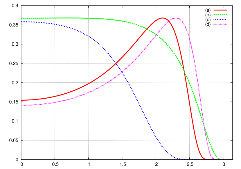
The integrands for the derivatives of $g_{\alpha}(x)$ and for the Mittag-Leffler case have similar aspects. They are all of the type $f_{n}=u^{n}e^{-u}$ on the interval $\varphi\in[0,\pi]$, where $u$ is given by Eq. (10). It is easy to show that: $f_{n}=u_{0}^{n}e^{-u_{0}}$ and $f^{\prime}_{n}=0$ for $\varphi=0$, with $u_{0}=(1-\alpha)(\alpha/x)^{\alpha/(1-\alpha)}$; $f_{n}\to 0$ for $\varphi\to\pi$; and that $f_{n}$ has a maximum for $\varphi$ such that $u=n$, provided $u_{0}<n$. Although the position of such maximum does depend on $\alpha$ and $x$, its value ($f_{n}=n^{n}e^{-n}$) depends only on $n$. For a given $\alpha$, larger values of $x$ displace the maximum towards $\varphi=\pi$, while smaller values does towards $\varphi=0$. If $u_{0}\geq n$, the unique maximum of $f_{n}$ is at $\varphi=0$. For the cumulative distribution function (18), the integrand corresponds to $n=0$. In particular its maximum is located at $\varphi=0$, with $f_{0}=1$, irrespective of the values of $x>0$ and $0<\alpha<1$. All these functions are well-behaved on the interval $\varphi\in[0,\pi]$ and, consequently, integrals like Eqs. (9), (18), (II), and (20) can be evaluated numerically without major problems.

We have set up an adaptive integration scheme based on the publicly available DQAGS routine of SLATEC slatec . We could integrate Eqs. (9), (18), (II), and (20) with little computational effort demanding a relative error in DQAGS smaller than $10^{-8}$, which is typically attained with about 10 iterations of the global adaptative scheme of the routine. Our FORTRAN code, available at html , has demonstrated to be extremely robust and reliable. In order to test it, we have used the case corresponding to the Lévy distribution with $\alpha=1/2$, for which an explicit form for the probability density function is known, namely the so-called Smirnov’s distribution

$$S(x)=g_{1/2}(x)=\frac{e^{-1/4x}}{2\sqrt{\pi}x^{3/2}}.$$ (21)

Fig. 2

Figure 2: Plots for $g_{1/2}(x)$ (a), $2\Lambda_{1/2}(x)$ (b), $(1/15)g^{\prime}_{1/2}(x)$ (c), and $(1/500)g^{\prime\prime}_{1/2}(x)$ (d), for $0\leq x\leq 1$, calculated by the numerical integration of Eqs. (9), (18), (II), and (20) by means of the SLATEC slatec adaptative integration routine DQAGS. The relative errors for all the four curves, calculated with respect to the exact Smirnov’s distribution (21) in the interval $0\leq x\leq 5$, are smaller than $3\times 10^{-8}$. (Numerical code available at html .)

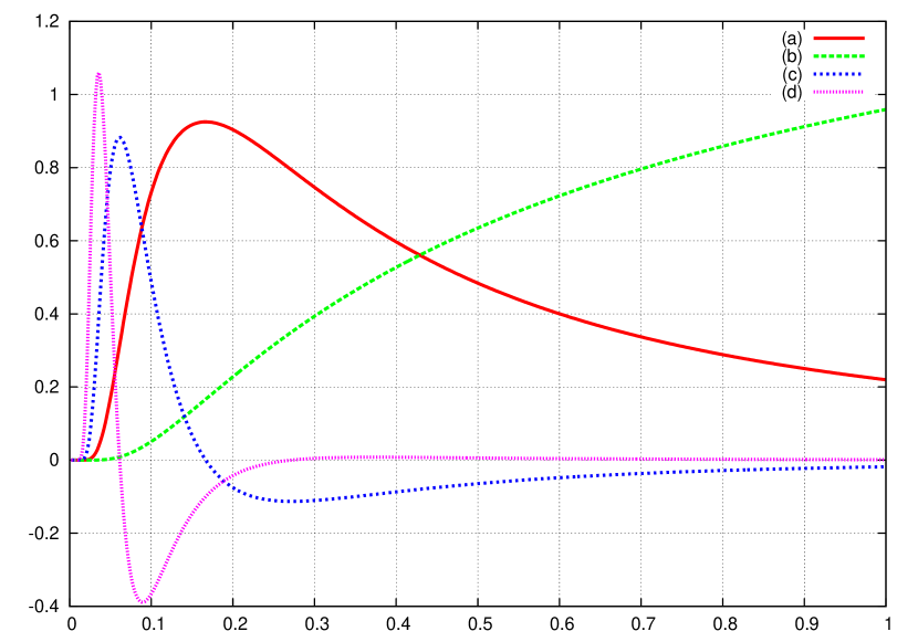
shows the functions $g_{1/2}(x)$, $\Lambda_{1/2}(x)$, $g^{\prime}_{1/2}(x)$, and $g^{\prime\prime}_{1/2}(x)$ evaluated numerically with our code. As we see, we can calculate $g_{\alpha}(x)$ with very good accuracy and in an efficient way. The corresponding data (500 points for each curve) for plots like those ones depicted in Fig. 2 are generated instantaneously in a Intel Core i7 computer. The relation (7) and the Smirnov’s distribution (21) allow us to test also the Mittag-Leffler case since they imply that

$$\rho_{1/2}(x)=\frac{e^{-x^{2}/4}}{\sqrt{\pi}}.$$ (22)

Our numerical procedure works with similar accuracy for this particular Mittag-Leffler probability density, with the usual caveats related to extremely small values of $x$ in (22), which correspond to large values of $x$ in $g_{1/2}(x)$ according to (7). We also checked the good accuracy of our algorithm by comparing the output with Nolan’s STABLE package Ref .

The numerical evaluation of the probability densities for extreme values of $x$ and $\alpha$ is quite delicate due to convergence and roundoff problems. For a fixed $\alpha$ and $x\to 0$ and $x\to\infty$, the asymptotic formulas (11), (12), (16), and (17) can be indeed used to estimate the probability densities. For fixed $x$ and $\alpha$ very close to $0$ and $1$, other asymptotic expressions are necessary. For small $\alpha$, we have from Eq. (10)

$$u\approx 1+\alpha\ln\alpha+\left(\ln\frac{\varphi}{x\sin\varphi}-\frac{\varphi}{\tan\varphi}\right)\alpha.$$ (23)

For a fixed $x\in(\alpha,1/\alpha)$, we have $u\approx 1+\alpha\ln\alpha$ for small enough $\alpha$ and $0\leq\varphi<\pi$, leading to $ue^{-u}\approx e^{-1}\left(1-(\alpha\ln\alpha)^{2}/2\right)$ for small $\alpha$ and $0\leq\varphi<\pi$. Applying these results in Eq. (9), one has

$$g_{\alpha}(x)\approx\frac{\alpha}{ex},$$ (24)

valid for small $\alpha$ and $\alpha<x<1/\alpha$. For $x<\alpha$, the approximation (11) is still valid for small $\alpha$. In particular, we always have $g_{\alpha}(x)\to 0$ for $x\to 0$, irrespective of the value for $\alpha$. Since the hypothesis of $\alpha<x<1/\alpha$ was explicitly used, the approximation (24) is not supposed to be accurate for $x\to\infty$. In this case, Eq. (12) is the correct asymptotic expression for $g_{\alpha}(x)$. For $\alpha$ close to $1$, the situation is a little bit more involved. Introducing $1-\alpha=\varepsilon>0$, we have from Eq. (10)

$$u\approx\frac{\varepsilon}{x^{1/\varepsilon}}\frac{\varphi}{\sin\varphi}e^{-\varphi/\tan\varphi},$$ (25)

valid for $\varepsilon\approx 0$, $0<x<\infty$, and $0\leq\varphi<\pi$. For $x>1$, $u\to 0$ for small $\varepsilon$, implying that $g_{1-\varepsilon}(x)\to 0$. For $x<1$, $u\to\infty$, also implying $g_{1-\varepsilon}(x)\to 0$. Since, according to Eq. (1), $g_{\alpha}(x)$ is supposed to be normalized for any value of $\alpha$, $g_{\alpha}(x)\to\infty$ for $x\to 1$ and $\alpha\to 1$. Hence, for $\alpha$ close to $1$, $g_{\alpha}(x)$ should be strongly peaked around $x=1$, resembling an approximation for a $\delta$-function. Such behavior could also be inferred by considering the limit $\alpha\to 1$ directly in Eq. (1).

II.1 The maxima of the distributions

As an application of our numerical procedures, we will explore some properties of the distribution $g_{\alpha}(x)$ and $\rho_{\alpha}(x)$. The location of the maxima of these probability density functions is certainly pertinent to the understanding of the statistical processes governed by them. Let us consider fist the case of $g_{\alpha}(x)$. The condition determining the location $x_{*}(\alpha)$ of the maximum of the probability density is, of course, $g^{\prime}_{\alpha}(x_{*})=0.$ From the approximations discussed in the preceding section, we have that $0<x_{*}(\alpha)<1$ for $0<\alpha<1$ and that $g_{\alpha}(x_{*})\to\infty$ for $\alpha\to 0$ and for $\alpha\to 1$. The zero of $g^{\prime}_{\alpha}(x)$ can be localized in the interval $(0,1)$ with a prescribed accuracy by using, for instance, a simple bisection method. Since we have a procedure to calculate $g^{\prime\prime}_{\alpha}(x)$, one could even implement a refinement for the determination of $x_{*}(\alpha)$ based, for instance, in Newton-Rapson method. Fig. 3 shows the values of $x_{*}(\alpha)$ and $g_{\alpha}(x_{*})$ for $0<\alpha<1$.

Figure 3: Location and value of the maxima of the probability density functions of Lévy (curves (a) and (b)) and Mittag-Leffler (curves (c) and (d)) distributions. Curves (a) and (c) correspond to the location $x_{*}(\alpha)$ of the maxima (left scale), as function of $\alpha\in(0,1)$ (horizontal axis). Curves (b) and (d) are the value of the maxima (right scale) as function of $\alpha$. The marked points correspond to the shortest maxima for each distribution, $(\alpha=0.567,g_{\alpha}(x_{*})=0.888)$ and $(\alpha=0.605,\rho_{\alpha}(x_{*})=0.509)$.

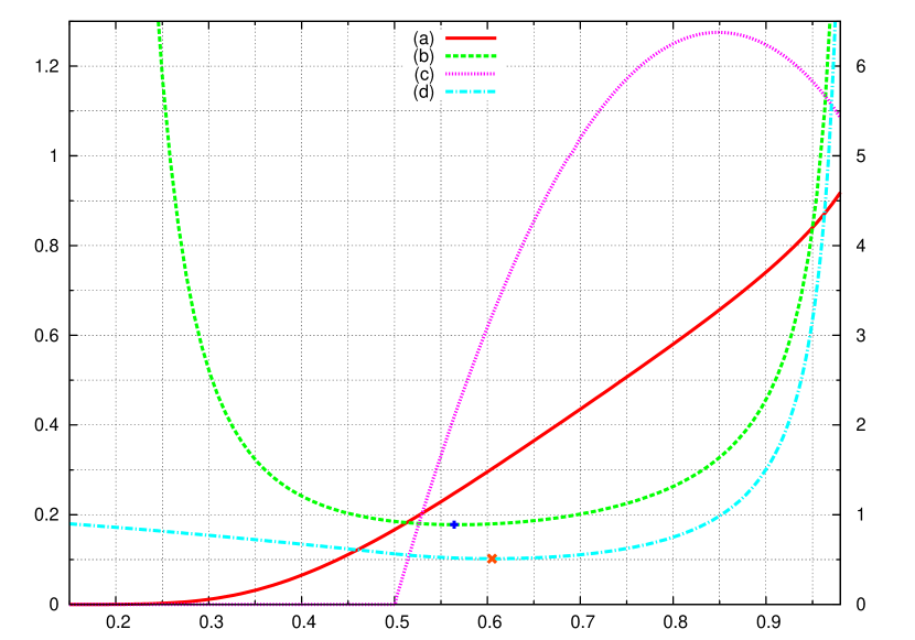
Notice that, as expected, we have that $g_{\alpha}(x_{*})\to\infty$ for $\alpha\to 0$ and $\alpha\to 1$, in agreement with the approximations of last section. The minimal value of $g_{\alpha}(x_{*})$ is attained when $\alpha=0.567$, corresponding to the one-sided $\alpha$-stable Lévy distribution with shortest maximum, for which $g_{\alpha}(x_{*})\approx 0.888$.

Figure 4: Lévy and Mittag-Leffler probability densities with shortest maxima (respectively, curves (a), with $\alpha=0.567$, and (c), with $\alpha=0.605$, see Fig. 3) and their respective cumulative distribution function (curves (b) and (d)) in the interval $0<x<3$.

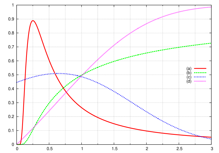
(Fig. 4).

The situation for $\rho_{\alpha}(x)$ is rather more involved. For $\alpha\approx 1$, $\rho_{\alpha}(x)$ is similar to $g_{\alpha}(x)$, both resembling approximations of a $\delta$-function around $x=1$. Such behavior for the Mittag-Leffler case can also be inferred directly from the definition (4), by considering the limit $\alpha\to 1$. However, in contrast with the previous case, for $\alpha\approx 0$, $\rho_{\alpha}(x)\approx e^{-x}$, as one can also see by evaluating the limit $\alpha\to 0$ in Eq. (4). Hence, for small $\alpha$, the maximum of $\rho_{\alpha}(x)$ located at $x=0$ and is given by $\rho_{\alpha}(0)\approx 1$. In fact, we could verify numerically that for $\alpha<1/2$, the maximum of $\rho_{\alpha}(x)$ is is always at $x=0$ and is given by Eq. (16). For $\alpha>1/2$, we have $\rho^{\prime}_{\alpha}(0)>0$ and the function $\rho_{\alpha}(x)$ attains a maximum for $x>0$ and then decays. Curiously, as $\alpha$ increases, $x_{*}(\alpha)$ also increases and even exceed $x=1$, and then return to $x=1$, but from the right-handed side. This behavior, which will be crucial for the discussion of the next section, is depicted by the curve (c) in Fig. 3. The Lévy and Mittag-Leffler distribution with shortest maxima are plotted in Fig. 4.

III Distribution of Lyapunov exponents in intermittent systems

We can also apply our numerical procedures to elucidate some dynamical problems of physical interest. This is the case, for instance, of the distribution of Lyapunov exponents in intermittent systems such as the Pomeau-Manneville maps $x_{t+1}=x_{t}+ax_{t}^{z}\,(\mbox{mod}\,1)$ considered recently in KB . For $z>2$, theses systems are known to exhibit, for nearby trajectories, a subexponential deviation of the type $\delta x_{t}\sim\delta x_{0}\exp(\lambda_{\alpha}t^{\alpha})$, where $\alpha=1/(z-1)$. According to the Aaronson-Darling-Kac (ADK) theorem ADK , for randomly distributed initial conditions and sufficiently large times, the ratio $\lambda_{\alpha}/\left\langle\lambda\right\rangle$, where $\left\langle\lambda\right\rangle$ is a suitable average for the exponents $\lambda_{\alpha}$, converges in distribution terms towards a Mittag-Leffler random variable with unit first moment and index $\alpha\in(0,1)$. Such statistics was also considered previously in Ref. AA from the numerical point of view. Some recent numerical works KB have reported a regular tendency of $\lambda_{\alpha}$ be smaller than the average $\left\langle\lambda\right\rangle$ for large values of $z$ (small $\alpha$). In fact, in KB the first moment $\left\langle\lambda\right\rangle$ is calculated differently from the ADK theorem, it is obtained there from a continuous-time stochastic model, but its values are, for the considered Pomeau-Manneville maps, the same of the ADK ones. Since $\lambda_{\alpha}/\left\langle\lambda\right\rangle$ is a random Mittag-Leffler variable, we can evaluate the probability of having $\lambda_{\alpha}<\left\langle\lambda\right\rangle$

$$\mbox{Prob}(\lambda_{\alpha}<\left\langle\lambda\right\rangle)=\int_{0}^{1}\rho^{(r)}_{\alpha}(x)dx=1-\Lambda_{\alpha}(\Gamma^{1/\alpha}(1+\alpha)),$$ (26)

where $r=\Gamma^{1/\alpha}(1+\alpha)$ assures that $\rho^{(r)}_{\alpha}(x)$ has unit fist moment, as required by the ADK theorem.

Figure 5: Curve (a): probability of having $\lambda_{\alpha}<\left\langle\lambda\right\rangle$ in Pomeau-Manneville maps as function of $\alpha\in(0,1)$, according to Eq. (26). The marked point ($\alpha\approx 0.747$) corresponds to the equiprobability. Detail: curves (b) and (c) are, respectively, the probability density of Mittag-Leffler distribution with unit first moment and $\alpha=0.1$ (left $y$-scale) and $\alpha=0.9$ (right $y$-scale) in the interval $0<x<3$. It is clear why the probability decays for increasing $\alpha$: the probability density tends towards a $\delta$-function centered in $x=1$, but from the right handed side. (See curve (c) in Fig. 3).

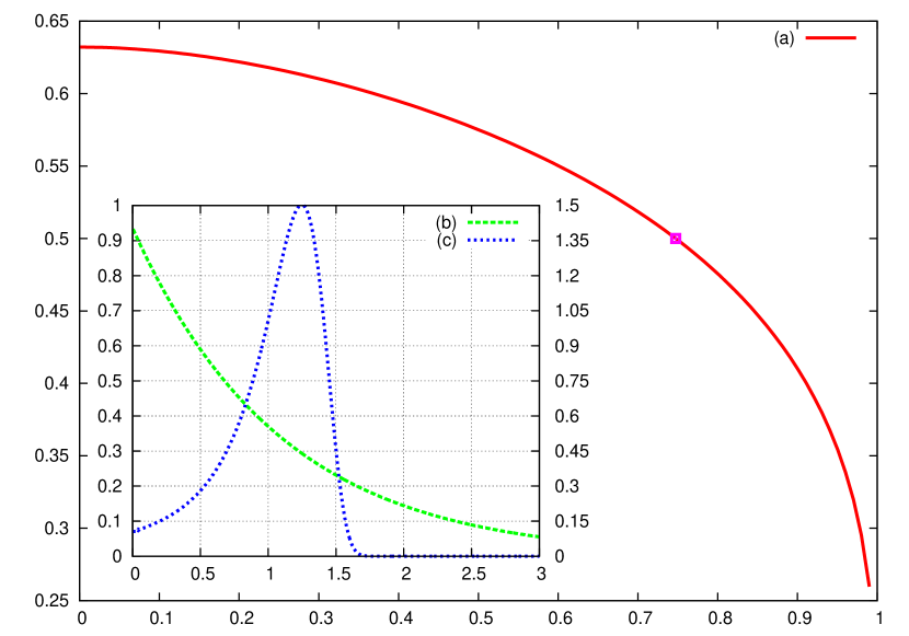
Fig. 5 depicts this probability as function of $\alpha$. For $\alpha\to 0$, we have $\mbox{Prob}(\lambda_{\alpha}<\left\langle\lambda\right\rangle)\to 1-1/e\approx 63\%$. As we see, the tendency reported in KB of having $\lambda_{\alpha}<\left\langle\lambda\right\rangle$ can be clearly understood from the ADK theorem. Moreover, the aspect of the Mittag-Leffler distributions for small $\alpha$ and $\alpha\to 1$ explains why these intermittent systems do exhibit such kind of behavior. For $\alpha\to 0$, the probability density function of the Mittag-Leffler distribution has the form $\rho_{\alpha}(x)\approx e^{-x}$ (See Fig. 5). Its maximum is located at $x=0$, and it is clear that the typical values of the random variable are always smaller than its average. On the other hand, for $\alpha\to 1$ ($z\to 2^{+}$), the probability density resembles a $\delta$-function with center approaching $x=1$, but from the right handed sided, see Fig. 5. In this case, the typical values of the random variable remain close the value of its average. Also from figure, we have that for $\alpha>3/4$ the probability of having $\lambda_{\alpha}>\left\langle\lambda\right\rangle$ is favorable over Eq. (26). (In fact, the equiprobability corresponds to $\alpha\approx 0.747$.) In terms of the distribution of Lyapunov exponents for the Pomeau-Manneville maps, this would correspond to have a slight predominance of $\lambda_{\alpha}$ greater than the average $\left\langle\lambda\right\rangle$ for small $z>2$. This seems, in fact, marginally evident from KB , but further work is necessary to establish this fact with the same certainty of the behavior for large $z$. This kind of problem in intermittent systems are very interesting and certainly deserve a deeper investigation.

IV Final remarks

Motivated by the closed form formulas in terms of the Meijer G-functions for the probability densities $g_{\alpha}(x)$ of one-sided Lévy distributions with rational $\alpha=l/k$ proposed by Penson and Górska in PG , we have introduced a numerical scheme for the computation of $g_{\alpha}(x)$ for any real $\alpha\in(0,1)$. By exploring the relation between one-sided Lévy and Mittag-Leffler distributions, we extend our procedures to include the evaluation of the the probability densities $\rho_{\alpha}(x)$ of Mittag-Leffler distributions. The main advantage of our numerical approximation is that it can be applied for any value $\alpha$, while Penson and Górska formula (2) is rather problematic for fractions with large denominators. As an application of our procedures, we determine the maximum location and value for the densities $g_{\alpha}(x)$ and $\rho_{\alpha}(x)$ as function of the index $\alpha\in(0,1)$. We show that $\alpha\approx 0.567$ and $\alpha\approx 0.605$ correspond, respectively, to the one-sided Lévy and Mittag-Leffler distributions with shortest maxima. Furthermore, we use our numerical procedure for the evaluation of Mittag-Leffler distribution to show that a recently described statistical behavior for intermittent systems KB , namely the predominance of having Lyapunov exponents $\lambda_{\alpha}$ smaller than the theoretical average $\langle\lambda\rangle$ for Pomeau-Manneville maps with large $z$, is nothing else than a consequence of the Mittag-Leffler statistics. We hope our numerical procedures could be useful for this kind of study.