Effect of coupling asymmetry on mean-field solutions of direct and inverse Sherrington-Kirkpatrick model

Abstract

We study how the degree of symmetry in the couplings influences the performance of three mean field methods used for solving the direct and inverse problems for generalized Sherrington-Kirkpatrick models. In this context, the direct problem is predicting the potentially time-varying magnetizations. The three theories include the first and second order Plefka expansions, referred to as naive mean field (nMF) and TAP, respectively, and a mean field theory which is exact for fully asymmetric couplings. We call the last of these simply MF theory. We show that for the direct problem, nMF performs worse than the other two approximations, TAP outperforms MF when the coupling matrix is nearly symmetric, while MF works better when it is strongly asymmetric. For the inverse problem, MF performs better than both TAP and nMF, although an ad hoc adjustment of TAP can make it comparable to MF. For high temperatures the performance of TAP and MF approach each other.

1 Introduction

Predicting the dynamical properties of a disordered system given a specific realisation of its parameters is an old and important problem in statistical mechanics. This is what one can call a direct problem. Apart from being important on its own, solving the direct problem is also a crucial step in solving the inverse problem: inferring the parameters of a system from measurements of its dynamics. With the rapid advance of methods for observing the dynamics of biological systems composed of many elements, the inverse problem has received a lot of recent attention. This line of research has allowed inferring functional and physical connections in neuronal networks [1, 2, 3, 4, 5], gene regulatory networks [6] and protein residue contacts [7].

A useful platform for studying the inverse problem is a dynamical version of the Sherrington-Kirkpatrick (SK) model: a set of $N$ classical spins, $s_{i}=\pm 1$ subject to a potentially time-varying external field $h_{i}(t)$ with couplings $J_{ij}$ between them and a stochastic update rule. In the direct problem one tries to predict the magnetizations $m_{i}(t)$ given the coupling and fields. In the inverse problem one does the opposite, i.e. one infers the couplings and the fields from measured magnetizations and correlations.

When the system is in equilibrium and the distribution of states follows the Boltzmann distribution, several approaches for both direct and inverse problems have been developed. These include both exact and approximate iterative algorithms, such as Boltzmann learning and Susceptibility propagation [8, 9] relating the magnetizations to model parameters, as well as closed-form equations based on naive mean field (nMF) and TAP [10, 11] equations for the SK model. Motivated by the fact that biological systems are usually out of equilibrium, some recent work has focused on reconstructing the parameters of a dynamical Ising spin glass model obeying either synchronous or asynchronous updating from observing its out-of-equilibrium dynamics [5, 12, 13].

In this paper, we investigate how three recently proposed mean field methods for the direct and inverse problems perform on models with different degrees of symmetry in their coupling matrices. The three methods are the nMF and TAP equations, derived using the high-temperature Plefka expansions of the generating functional to first order and second order [14], and a mean field theory (denoted simply MF) [13] that is exact for the SK model with fully asymmetric couplings.

2 Solutions to the direct and inverse problems

We consider a model in which the probability of being in state $\mathbf{s}$ at time step $t$, $p_{t}(\mathbf{s})$, is given by

$$p_{t+1}(\mathbf{s})=\sum_{\mathbf{s}^{\prime}}W_{t}[\mathbf{s};\mathbf{s}^{\prime}]p_{t}(\mathbf{s}^{\prime})$$ (1a)

$$W_{t}[\mathbf{s};\mathbf{s}^{\prime}]=\prod_{i}\frac{\exp(s_{i}\theta_{i})}{2\cosh\theta_{i}}$$ (1b)

$$\theta_{i}(t)=h_{i}(t)+\sum_{j}J_{ij}s^{\prime}_{j}(t).$$ (1c)

For the choice of couplings $J_{ij}$, we follow [15], taking

$$J_{ij}=J^{sym}_{ij}+kJ^{asym}_{ij}$$ (2)

where $J^{sym}_{ij}=J^{sym}_{ji}$ is the symmetric part of the couplings while $J^{asym}_{ij}=-J^{asym}_{ji}$ is the antiymmetric part. All the couplings $J^{sym}_{ij}$ and $J^{asym}_{ij}$ are drawn independently from a zero-mean Gaussian distribution with variance

$$\overline{[J^{symm}_{ij}]^{2}}=\overline{[J^{asym}_{ij}]^{2}}=\frac{g^{2}}{(1+k^{2})N}.$$ (3)

With Eqs. 2 and 3, the couplings $J_{ij}$ have variance of $g^{2}/N$ and the degree of symmetry is controlled by $k$: for $k=0$ the model is fully symmetric ($J_{ij}=J_{ji}$) while for $k=1$, it is fully asymmetric ($J_{ij}$ independent of $J_{ji}$).

The direct problem consists in estimating the instantaneous magnetization of spin $i$ at time $t$, $m_{i}(t)$. The estimation obtained from the nMF, TAP and MF are respectively:

$$m_{i}(t+1)=\tanh\Big{[}h_{i}(t)+\sum_{j}J_{ij}m_{j}(t)\Big{]}$$ (4a)

$$m_{i}(t+1)=\tanh\Big{[}h_{i}(t)+\sum_{j}J_{ij}m_{j}(t)-m_{i}(t+1)\sum_{j}J^{2}_{ij}(1-m_{j}^{2}(t))\Big{]}$$ (4b)

$$m_{i}(t+1)=\int\frac{dx}{\sqrt{2\pi}}e^{-x^{2}/2}\tanh\Big{[}h_{i}(t)+\sum_{j}J_{ij}m_{j}(t)+x\sqrt{\Delta_{i}(t)}\Big{]}$$ (4c)

where in the last equation

$$\Delta_{i}(t)=\sum_{j}J_{ij}^{2}(1-m_{i}^{2}(t))\ .$$ (5)

For deriving Eqs. 4a and 4b, i.e. nMF and TAP, one first writes down the generating functional for the process defined by Eq. 1c, performs a Legendre transform to fix the magnetizations and expands the results for small $g$ (i.e. high temperature). To the first order, this expansion gives the nMF equations, Eq. 4a. Keeping terms up to the second order yields a correction to the nMF equations resulting in the the TAP equations, Eq. 4b, for this dynamical model. nMF and TAP are, therefore, high temperature expansions for an arbitrary set of couplings, with no assumption about their distribution or its degree of symmetry. The third equation is derived for arbitrary $g$, but under the mean-field assumption that at each time step the fields acting on the spins are independent Gaussian variables. This is exact for this SK model when the coupling matrix is fully asymmetric i.e. when $k=1$.

These direct equations can also be used for solving the inverse problem. The idea is to use the data in order to measure the magnetizations $m_{i}(t)$, the equal time correlations $C_{ij}=\langle\delta s_{i}(t)\delta s_{j}(t)\rangle$, and the time-delayed correlations $D_{ij}=\langle\delta s_{i}(t+1)\delta s_{j}(t)\rangle$, where $\delta s_{i}(t)=s_{i}(t)-m_{i}(t)$. For the process in Eq. 1c, one can write the time-delayed correlations as

$$D_{ij}=\langle\tanh\big{[}\theta_{i}(t)\big{]}s_{j}(t)\rangle-\langle\tanh\big{[}\theta_{i}(t)\big{]}\rangle\langle s_{j}(t)\rangle.$$ (6)

To derive the inverse TAP and nMF, one then uses Eq. 6, expands the $\tanh$ around $m_{i}$ that satisfies one of the direct equations 4a and 4b. In the case of MF, one writes an expression for the joint distribution of $\theta_{i}(t)$ and $\theta_{j}(t)$ that is exact for a fully asymmetric SK model. This joint distribution can then be used to relate $\mathbf{J}\mathbf{D}$ to $\mathbf{C}$ in the limit of small $C_{ij}$; for details see [5, 13]. Within all three approximations, nMF, TAP, and MF, the resulting expression takes the form

$$\mathbf{D}=\mathbf{A}\mathbf{J}\mathbf{C}\ ,$$ (7)

where the matrix $A$ is a diagonal matrix that depends on the approximation:

$$A^{\rm nMF}_{ij}=\delta_{ij}(1-m_{i}^{2})\ ,$$ (8a)

$$A^{\rm TAP}_{ij}=\delta_{ij}(1-m_{i}^{2})(1-F_{i})\ ,$$ (8b)

$$A^{\rm MF}_{ij}=\delta_{ij}\int\frac{dx}{\sqrt{2\pi}}e^{-x^{2}/2}\Big{[}1-\tanh^{2}(h_{i}(t)+\sum_{j}J_{ij}m_{j}+x\sqrt{\Delta_{i}})\Big{]}\ .$$ (8c)

In Eq. 8b $F_{i}$ satisfies a cubic equation. For details see [5] and [13]. Not surprisingly, expanding Eq. 8c to linear or second order in $J_{ij}$ yields $A^{\rm nMF}$ and $A^{\rm TAP}$ in Eqs. 8a and 8b, respectively.

Eq. 7 can be solved for $\mathbf{J}=\mathbf{A}^{-1}\mathbf{D}\mathbf{C}^{-1}$, provided one has enough data so that the estimation of $C$ is good, allowing its numerical inversion.

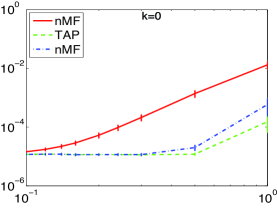
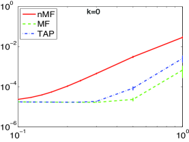
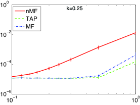
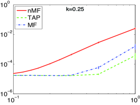
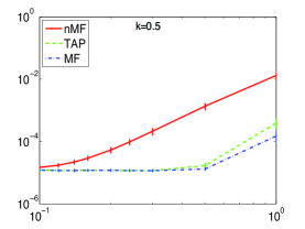
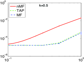
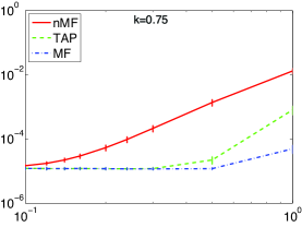
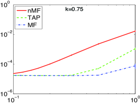
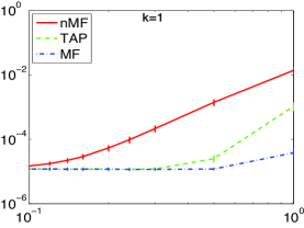
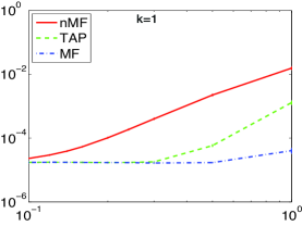
Figure 1: LEFT PANELS: Mean squared error of the three methods for predicting the magnetizations at time $t$ given at time $t-1$, averaged over spins and times, $\overline{(m_{i}^{\text{predicted}}(t)-m_{i}^{\text{measured}}(t))^{2}}$. This mean squared error is plotted as a function of $g$ for a system of size $N=50$ with a temporally constant field drawn independently for each spin from a normal distribution. We have used $100$ time steps and $50000$ repeats to calculate the experimental magnetizations and have averaged the errors over $10$ realizations of the couplings. The different figures correspond to different values of $k$. From top to bottom $k=0,0.25,0.5,0.75,1$. RIGHT PANELS: The same but with the addition of a sinusoidal external field of period $10$ time steps and amplitude $0.5$.

3 Effect of Symmetry

As mentioned before, for the direct problem, we expect that the MF becomes exact for $k=1$ for any coupling strength $g$. TAP equations should also become exact for $k=0$ in the limit of weak couplings. This is shown in Fig. 1, where we plot the mean squared error in predicting the magnetizations at time $t+1$ given the magnetizations at time $t$. This is done both for a constant field and for an external field that varies sinusoidally with time. As can be seen in this figure, for both types of external fields, TAP equations outperform the other two methods for small $k$. As temperature is increased, all three approximations perform better and become almost equally good. As $k$ increases, MF wins over TAP while nMF performs worse than both of them.

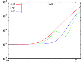
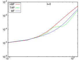
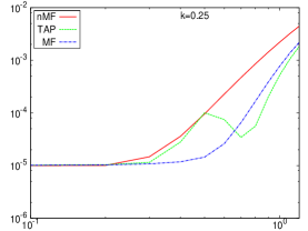
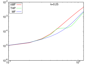
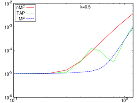
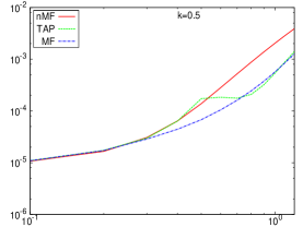
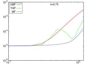
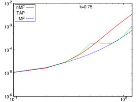
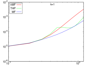
Figure 2: LEFT PANELS: Mean squarre error of the three methods on the infered couplings $\overline{(J_{ij}^{\text{infered}}-J_{ij}^{\text{real}})^{2}}$ as a function of $g$ for systems of size $N=100$ with zero external field, given $P=100000$ patterns, averaged over $10$ realizations of the couplings. The different figures correspond to different values of $k$. From top to bottom $k=0,0.25,0.5,0.75,1$. RIGHT PANELS: The same but with the addition of a sinusoidal external field of period $10$ time steps and amplitude $0.5$.

The situation for the inverse problem is slightly more complicated. This is because, for strong couplings, the cubic equation that $F_{i}$ solves develops complex roots. In this case one can take three approaches: (i) take the nMF result, (ii) take the real part of the solution, (iii) take the solution for the largest $g$ for which the solutions are real. This value can be shown to be $F_{i}=1/3$. The results for the last two strategies almost coincide, with strategy (iii) performing slightly better in lower temperatures, so we chose this one. In strategy (i) the results just coincide with the nMF approach after the temperature at which the cubic equation for $F_{i}$ develops complex roots. The results from strategy (iii) are shown in Fig. 2. It is clear from this figure that nMF always performs worse than the other two and that the difference between the three methods vanishes in the high-temperature limit. On the other hand, MF is superior, as expected, when one gets closer to the asymmetric case i.e. for $k$ is close to 1. The TAP result has a more complicated behavior, due to the intrinsic limitations imposed by the lack of real solutions of the cubic equation at strong couplings. However, one can notice that, when $k$ is close to zero, there is a range of couplings $g$ where TAP becomes better than MF as it is expected.

As can be seen in the right column of Fig. 2, the mean squared error $\overline{(J_{ij}^{\text{infered}}-J_{ij}^{\text{real}})^{2}}$ becomes larger for non-zero external fields. This is a general feature of all three methods. Large fields and/or couplings are estimated with larger errors than small ones. This is because errors in the estimation of the empirical magnetizations/correlations, when the later are close to $\pm 1$, produce large errors in the estimation of the fields/couplings (consider for example, in zeroth order approximation, a sigmoid map between $m_{i}$ and $h_{i}$ , and $c_{ij}$ and $J_{ij}$). Numerical simulations show that, for large external field amplitude, these errors become so important that the differences between the three methods are insignificant.

4 Conclusions

Within the mean field approaches that we have studied, the solution of the inverse problem derives from the solution of the direct problem. We have studied here three methods that provide an approximate solution to the direct problem in the case of systems with infinite range interactions. We have explored their behaviors on both the direct and the inverse problem in the case of SK models with different degrees of symmetry of the interactions. As expected, the MF approach is the best one when the degree of asymmetry is large enough, but the TAP approach turns out to be slightly better in some range of coupling strength when the couplings are more symmetric. The nMF approach is just a first order approximation to both MF and TAP and is systematically worse than the other two methods.

As noted before, the derivation of inverse nMF and TAP rely on expanding the $\tanh$ in the around the solutions of the nMF and TAP. This expansion is not required for the MF solution: in the case with the assumption of full asymmetry, the joint distribution of the local field to each pair of spins will be Gaussian and can be easily calculated. It is therefore possible to write an exact equation relating $D_{ij}$ to $C_{ij}$ and the couplings which in the limit of small $C_{ij}$ can be linearized and takes the form of Eq. 7. It would be interesting to see if a similar approach can be done within the TAP framework: calculate the joint distribution of the local fields in a systematic small coupling expansion, and use the same procedure done in MF to relate $D_{ij}$ to $C_{ij}$.

In real applications, for instance in neural data analysis or gene regulation network reconstruction, one does not deal with data generated from a model with the particular size dependence of the couplings of the SK model. Our previous work shows that TAP and nMF perform at the same level in identifying the connections of a simulated neural network, and they both perform worse than the exact iterative Boltzmann like learning rule that one can write down for the dynamical SK model [5, 16]. We will leave the comparison of TAP, MF and the exact learning on biological data to future work.

References

- [1] E. Schneidman, M.J. Berry, R. Segev, and W. Bialek. Weak pairwise correlations imply strongly correlated network states in a neural population. Nature, 440:1007–1012, 2006.
- [2] J. Shlens, G.D. Field, J.L. Gauthier, M.I. Grivich, D. Petrusca, A. Sher, A.M. Litke, and E.J. Chichilnisky. The structure of multi-neuron firing patterns in primate retina. J. Neurosci., 26:8254–8266, 2006.
- [3] S. Cocco, S. Leibler, and R. Monasson. Neuronal couplings between retinal ganglion cells inferred by efficient inverse statistical physics methods. Proc Natl Acad Sci U S A, 106:14058–62, 2009.
- [4] Y. Roudi, S. Nirenberg, and P. E. Latham. Pairwise maximum entropy models for studying large biological systems: when they can work and when they can’t. PLoS Comput Biol, 5:e1000380, 2009.
- [5] Y. Roudi and J. Hertz. Mean field theory for nonequilibrium network reconstruction. Phys. Rev. Lett., 106:048702, 2011.
- [6] T. R. Lezon, J. R. Banavar, M. Cieplak, A. Maritan, and N. Fedoroff. Using the principle of entropy maximization to infer genetic interaction networks from gene expression patterns. Proc. Natl. Acad. Sci. USA, 103, 2006.
- [7] Martin Weigt, Robert A. White, Hendrik Szurmant, James A. Hoch, and Terence Hwa. Identification of direct residue contacts in protein-protein interaction by message passing. PNAS, 106:67–72, 2009.
- [8] Erik Aurell Charles Ollion and Yasser Roudi. Dynamics and performance of susceptibility propagation on synthetic data. Eur. Phys. J. B, 77:587–595, 2010.
- [9] Marc Mézard and Thierry Mora. Constraint satisfaction problems and neural networks: A statistical physics perspective. Journal of Physiology-Paris, 103:107–113, 2009.
- [10] T. Tanaka. Mean-field theory of boltzmann machine learning. Phys. Rev. E, 58:2302–2310, 1998.
- [11] H. J. Kappen and F. B. Rodriguez. Efficient learning in boltzmann machines using linear response theory. Neur. Comp., 10:1137–1156, 1998.
- [12] H.-L. Zeng, M. Alava, H. Mahmoudi, and E. Aurell. Network inference using asynchronously updated kinetic ising model. Phys. Rev. E, 83:041135, 2011.
- [13] M. Mezard and J. Sakellariou. Exact mean field inference in asymmetric kinetic ising systems. arXiv:1103.3433v2, 2011.
- [14] Y. Roudi and J. Hertz. Dynamical tap equations for non-equilibrium ising spin glasses. J. Stat. Mech., page P03031, 2011.
- [15] A. Crisanti and H. Sompolinsky. Dynamics of spin systems with randomly asymmetric bonds: Langevin dynamics and a spherical model. Phys. Rev. A, 36:4922–4939, 1987.
- [16] J. A. Hertz, Y. Roudi, A. Thorning, J. Tyrcha, E. Aurell, and H-L. Zeng. Inferring network connectivity using kinetic ising models. BMC Neuroscience, 10, 2010.