Physarum Can Compute Shortest Paths

Abstract

Physarum Polycephalum is a slime mold that is apparently able to solve shortest path problems. A mathematical model has been proposed by biologists to describe the feedback mechanism used by the slime mold to adapt its tubular channels while foraging two food sources $s_{0}$ and $s_{1}$. We prove that, under this model, the mass of the mold will eventually converge to the shortest $s_{0}$-$s_{1}$ path of the network that the mold lies on, independently of the structure of the network or of the initial mass distribution.

This matches the experimental observations by the biologists and can be seen as an example of a “natural algorithm”, that is, an algorithm developed by evolution over millions of years.

1 Introduction

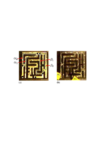
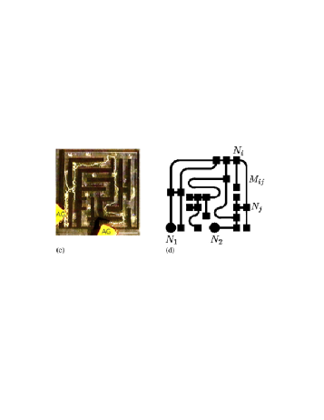
Figure 1: The experiment in [NYT00] (reprinted from there): (a) shows the maze uniformly covered by Physarum; the yellow color indicates the presence of Physarum. Food (oatmeal) is provided at the locations labelled AG. After a while, the mold retracts to the shortest path connecting the food sources as shown in (b) and (c). (d) shows the underlying abstract graph. The video [You10] shows the experiment.

Physarum Polycephalum is a slime mold that is apparently able to solve shortest path problems. Nakagaki, Yamada, and Tóth [NYT00] report on the following experiment, see Figure 1: They built a maze, covered it with pieces of Physarum (the slime can be cut into pieces that will reunite if brought into vicinity), and then fed the slime with oatmeal at two locations. After a few hours, the slime retracted to a path that follows the shortest path connecting the food sources in the maze. The authors report that they repeated the experiment with different mazes; in all experiments, Physarum retracted to the shortest path. There are several videos available on the web that show the mold in action [You10].

Paper [TKN07] proposes a mathematical model for the behavior of the slime and argues extensively that the model is adequate. We will not repeat the discussion here but only define the model. Physarum is modeled as an electrical network with time varying resistors. We have a simple undirected graph $G=(N,E)$ with distinguished nodes $s_{0}$ and $s_{1}$, which model the food sources. Each edge $e\in E$ has a positive length $L_{e}$ and a positive diameter $D_{e}(t)$; $L_{e}$ is fixed, but $D_{e}(t)$ is a function of time. The resistance $R_{e}(t)$ of $e$ is $R_{e}(t)=L_{e}/D_{e}(t)$. We force a current of value 1 from $s_{0}$ to $s_{1}$. Let $Q_{e}(t)$ be the resulting current over edge $e=(u,v)$, where $(u,v)$ is an arbitrary orientation of $e$. The diameter of any edge $e$ evolves according to the equation

$$\dot{D_{e}}(t)=|Q_{e}(t)|-D_{e}(t),$$ (1)

where $\dot{D_{e}}$ is the derivative of $D_{e}$ with respect to time. In equilibrium ($\dot{D_{e}}=0$ for all $e$), the flow through any edge is equal to its diameter. In non-equilibrium, the diameter grows or shrinks if the absolute value of the flow is larger or smaller than the diameter, respectively. In the sequel, we will mostly drop the argument $t$ as is customary in the treatment of dynamical systems.

The model is readily turned into a computer simulation. In an electrical network, every vertex $v$ has a potential $p_{v}$; $p_{v}$ is a function of time. We may fix $p_{s_{1}}$ to zero. For an edge $e=(u,v)$, the flow across $e$ is given by $(p_{u}-p_{v})/R_{e}$. We have flow conservation in every vertex except for $s_{0}$ and $s_{1}$; we inject one unit at $s_{0}$ and remove one unit at $s_{1}$. Thus,

$$b_{v}=\sum_{u\in\delta(v)}\frac{p_{v}-p_{u}}{R_{uv}},$$ (2)

where $\delta(v)$ is the set of neighbors of $v$ and $b_{s_{0}}=1$, $b_{s_{1}}=-1$, and $b_{v}=0$ otherwise. The node potentials can be computed by solving a linear system (either directly or iteratively). Tero et al. [TKN07] were the first to perform simulations of the model. They report that the network always converges to the shortest $s_{0}$-$s_{1}$ path, i.e., the diameters of the edges on the shortest path converge to one, and the diameters on the edges outside the shortest path converge to zero. This holds true for any initial condition and assumes the uniqueness of the shortest path.

Miyaji and Ohnishi [MO07, MO08] initiated the analytical investigation of the model. They argued convergence against the shortest path if $G$ is a planar graph and $s_{0}$ and $s_{1}$ lie on the same face in some embedding of $G$.

Our main result is a convergence proof for all graphs. For a network $G=(V,E,s_{0},s_{1},L)$, where $(L_{e})_{e\in E}$ is a positive length function on the edges of $G$, we use $G_{0}=(V,E_{0})$ to denote the subgraph of all shortest source-sink paths, $L^{*}$ to denote the length of a shortest source-sink path, and $\cal E^{*}$ to denote the set of all source-sink flows of value one in $G_{0}$. If we define the cost of flow $Q$ as $\sum_{e}L_{e}Q_{e}$, then $\cal E^{*}$ is the set of minimum cost source-sink flows of value one. If the shortest source-sink path is unique, $\cal E^{*}$ is a singleton. The dynamics are attracted by a set $A\subseteq\mathbb{R}^{E}$ if the distance (measured in any $L_{p}$-norm) between $D(t)$ and $A$ converges to zero.

Theorem [Theorem 2 in Section 6] Let $G=(V,E,s_{0},s_{1},L)$ be an undirected network with positive length function $(L_{e})_{e\in E}$. Let $D_{e}(0)>0$ be the diameter of edge $e$ at time zero. The dynamics (1) are attracted to $\cal E^{*}$. If the shortest source-sink path is unique, the dynamics converge to the flow of value one along the shortest source-sink path.

We conjecture that the dynamics converge to an element of $\cal E^{*}$ but only show attraction to $\cal E^{*}$. A key part of our proof is to show that the function

$$V=\frac{1}{\min_{S\in{\cal C}}C_{S}}\sum_{e\in E}L_{e}D_{e}+(C_{\{s_{0}\}}-1)^{2}$$ (3)

decreases along all trajectories that start in a non-equilibrium configuration. Here, ${\cal C}$ is the set of all $s_{0}$-$s_{1}$ cuts, i.e., the set of all $S\subseteq N$ with $s_{0}\in S$ and $s_{1}\not\in S$; $C_{S}=\sum_{e\in\delta(S)}D_{e}$ is the capacity of the cut $S$ when the capacity of edge $e$ is set to $D_{e}$; and $\min_{S\in{\cal C}}C_{S}$ (also abbreviated by $C$) is the capacity of the minimum cut. The first term in the definition of $V$ is the normalized hardware cost; for any edge, the product of its length and its diameter may be interpreted as the hardware cost of the edge; the normalization is by the capacity of the minimum cut. We will show that the first term decreases except when the maximum flow $F$ in the network with capacities $D_{e}$ is unique, and moreover, $|Q_{e}|=|F_{e}|/C$ for all $e$. The second term decreases as long as the capacity of the cut defined by $s_{0}$ is different from 1. We show that the capacity of the minimum cut converges to one and that the derivative of $V$ is upper bounded by $-\sum_{e}(L_{\mathrm{min}}/4)(D_{e}/C-|Q_{e}|)^{2}$, where $L_{\mathrm{min}}$ is the minimum length of any edge. Since $V$ is non-negative, this will allow us to conclude that $|D_{e}-|Q_{e}||$ converges to zero for all $e$. In the next step, we show that the potential difference $\Delta=p_{s_{0}}-p_{s_{1}}$ between source and sink converges to the length $L^{*}$ of a shortest-source sink path. We use this to conclude that $D_{e}$ and $Q_{e}$ converge to zero for any edge $e\not\in E_{0}$. Finally, we show that the dynamics are attracted by $\cal E^{*}$.

We found the function $V$ by analytical investigation of a network of parallel links (see Section 4), extensive computer simulations, and guessing. Functions decreasing along all trajectories are called Lyapunov functions in dynamical systems theory [HS74]. The fact that the right-hand side of system (1) is not continuously differentiable and that the function $V$ is not differentiable everywhere introduces some technical difficulties.

The direction of the flow across an edge depends on the initial conditions and time. We do not know whether flow directions can change infinitely often or whether they become ultimately fixed. Under the assumption that flow directions stabilize, we can characterize the (late stages of the) convergence process. An edge $e=\{u,v\}$ becomes horizontal if $\lim_{t\to\infty}|p_{u}-p_{v}|=0$, and it becomes directed from $u$ to $v$ (directed from $v$ to $u$) if $p_{u}>p_{v}$ for all large $t$ ($p_{v}>p_{u}$ for all large $t$). An edge stabilizes if it either becomes horizontal or directed, and a network stabilizes if all its edges stabilize. If a network stabilizes, we partition its edges into a set $E_{h}$ of horizontal edges and a set $\overrightarrow{E}$ of directed edges. If $\{u,v\}$ becomes directed from $u$ to $v$, then $(u,v)\in\overrightarrow{E}$.

We introduce the notion of a decay rate. Let $r\leq 0$. A quantity $D(t)$ decays with rate at least $r$ if for every $\varepsilon>0$ there is a constant $A$ such that $\ln D(t)\leq A+(r+\varepsilon)t$ for all $t$. A quantity $D(t)$ decays with rate at most $r$ if for every $\varepsilon>0$ there is a constant $a$ such that $\ln D(t)\geq a+(r-\varepsilon)t$ for all $t$. A quantity $D(t)$ decays with rate $r$ if it decays with rate at least and at most $r$.

Lemma [Lemma 20 in Section 7] For $e\in E_{h}$, $D_{e}$ decays with rate $-1$ and $|Q_{e}|$ decays with rate at least $-1$.

\psfrag{e1}{$e_{1}$}\psfrag{e2}{$e_{2}$}\psfrag{e3}{$e_{3}$}\psfrag{e4}{$e_{4}$}\psfrag{e5}{$e_{5}$}\psfrag{e6}{$e_{6}$}\psfrag{s0}{$s_{0}$}\psfrag{s1}{$s_{1}$}\psfrag{u}{$u$}\psfrag{v}{$v$}\psfrag{w}{$w$}\includegraphics[width=173.44534pt]{pathdecomposition.eps}
(a)		(b)

Figure 2: Part (a) illustrates the path decomposition. All edges are assumed to have length 1; $P_{0}=(e_{1})$, $P_{1}=(e_{2},e_{3},e_{4})$, $P_{2}=(e_{5},e_{6})$, $p^{*}_{s_{0}}=1$, $p^{*}_{s_{1}}=0$, $p^{*}_{v}=1/3$, $p^{*}_{u}=2/3$, $p^{*}_{w}=1/2$, $f(P_{1})=1/3$, and $f(P_{2})=1/6$.
Part (b) shows the Wheatstone graph. The direction of the flow on edge $\{u,v\}$ may change over time; the flow on all other edges is always from left to right.

We define a decomposition of $G$ into paths $P_{0}$ to $P_{k}$, an orientation of these paths, a slope $f(P_{i})$ for each $P_{i}$, a vertex labelling $p^{*}$, and an edge labelling $r$. $P_{0}$ is a shortest $s_{0}$-$s_{1}$ path in $G$, $f(P_{0})=1$, $r_{e}=f(P_{0})-1$ for all $e\in P_{0}$, and $p_{v}^{*}=\mathrm{dist}(v,s_{1})$ for all $v\in P_{0}$, where $\mathrm{dist}(v,s_{1})$ is the shortest path distance from $v$ to $s_{1}$. For $1\leq i\leq k$, we have $P_{i}=\mathop{\mathrm{missing}}{argmax}_{P\in\cal P}f(P)$, where $\cal P$ is the set of all paths $P$ in $G$ with the following properties: (1) the startpoint $a$ and the endpoint $b$ of $P$ lie on $P_{0}\cup\ldots\cup P_{i-1}$, $p^{*}_{a}\geq p_{b}^{*}$, and $f(P)=(p_{a}^{*}-p_{b}^{*})/L(P)$; (2) no interior vertex of $P$ lies on $P_{0}\cup\ldots\cup P_{i-1}$; and (3) no edge of $P$ belongs to $P_{0}\cup\ldots\cup P_{i-1}$. If $p^{*}_{a}>p_{b}^{*}$, we direct $P_{i}$ from $a$ to $b$. If $p^{*}_{a}=p^{*}_{b}$, we leave the edges in $P_{i}$ undirected. We set $r_{e}=f(P_{i})-1$ for all edges of $P_{i}$, and $p^{*}_{v}=p^{*}_{b}+f(P_{i})\,\mathrm{dist}_{P_{i}}(v,b)$ for every interior vertex $v$ of $P_{i}$. Figure 2(a) illustrates the path decomposition.

Lemma [Lemma 21 in Section 7] There is an $i_{0}\leq k$ such that

$$f(P_{0})>f(P_{1})>\ldots>f(P_{i_{0}})>0=f(P_{i_{0}+1})=\ldots=f(P_{k}).$$

Theorem [Theorem 3 in Section 7] If a network stabilizes, $\overrightarrow{E}=\cup_{i\leq i_{0}}E(P_{i})$, the orientation of any edge $e\in\overrightarrow{E}$ agrees with the orientation induced by the path decomposition, and $E_{h}=\cup_{i>i_{0}}E(P_{i})$. The potential of each node $v$ converges to $p^{*}_{v}$. The diameter of each edge $e\in E\setminus P_{0}$ decays with rate $r_{e}$.

We cannot prove that flow directions stabilize in general. For series-parallel graphs, flow directions trivially stabilize. The Wheatstone graph, shown in Figure 2(b), is the simplest graph, in which flow directions may change over time.

Theorem [Theorem 6 in Section 8] The Wheatstone graph stabilizes.

The uncapacitated transportation problem generalizes the shortest path problem. With each vertex $v$, a supply/demand $b_{v}$ is associated. It is assumed that $\sum_{v}b_{v}=0$. Nodes with positive $b_{v}$ are called supply nodes, and nodes with negative $b_{v}$ are called demand nodes. In the shortest path problem, exactly two vertices have non-zero supply/demand. A feasible solution to the transportation problem is a flow $f$ satisfying the mass balance constraints, i.e., for every vertex $v$, $b_{v}$ is equal to the net flow out of $v$. The cost of a solution is $\sum_{e}L_{e}f_{e}$. The Physarum solver for the transportation problem is as follows: At any fixed time, the potentials are defined by (2) and the currents $(Q_{e})_{e\in E}$ are derived from the potentials by Ohm’s law. The dynamics evolve according to (1). The equilibria, i.e., $|Q_{e}|=D_{e}$ for all $e$, are precisely the flows with the following equal-length property. Orient the edges in the direction of $Q$ and drop the edges of flow zero. In the resulting graph, any two distinct directed paths with the same source and sink have the same length. Let $\cal E$ be the set of equilibria.

Theorem [Theorem 8 in Section 9] The dynamics (1) are attracted to the set of equilibria $\cal E$. If any two equilibria have distinct cost, the dynamics converge to an optimum solution of the transportation problem.

The convergence statement for the transportation problem is weaker than the corresponding statement for the shortest path problem in two respects. There, we show attraction to the set of equilibria of minimum cost (now only to the set of equilibria) and convergence to the optimum solution if the optimum solution is unique (now only if no two equilibria have the same cost).

This paper is organized as follows: In Section 2, we discuss related work, and in Section 3, we put our results into the context of natural algorithms and state open problems. The technical part of the paper starts in Section 4. We first treat a network of parallel links; this situation is simple enough to allow an analytical treatment. In Section 5, we review basic facts about electrical networks and prove some simple facts about the dynamics of Physarum. In Section 6, we prove our main result, the convergence for general graphs. In Section 7, we prove exponential convergence under the assumption that flow directions stabilize, and in Section 8, we show that the Wheatstone network stabilizes. Finally, in Section 9, we generalize the convergence proof to the transportation problem.

2 Related Work

Miyaji and Ohnishi [MO07, MO08] initiated the analytical investigation of the model. They argued convergence against the shortest path if $G$ is a planar graph and $s_{0}$ and $s_{1}$ lie on the same face in some embedding of $G$. Ito et al. [IJNT11] study the dynamics (1) in a directed graph $G=(V,E)$; they do not claim that the model is justified on biological grounds. Each directed edge $e$ has a diameter $D_{e}$. The node potentials are again defined by the equations

$$b_{v}=\sum_{u\in\delta(v)}\frac{p_{v}-p_{u}}{R_{uv}}\quad\text{for all $v\in V$}.$$

The summation on the right-hand side is over all neighbors $u$ of $v$; edge directions do not matter in this equation. If there is an edge from $u$ to $v$ and an edge from $v$ to $u$, $u$ occurs twice in the summation, once for each edge. The dynamics for the diameter of the directed edge $uv$ are then $\dot{D}_{uv}=Q_{uv}-D_{uv}$, where $Q_{uv}=D_{uv}(p_{u}-p_{v})/L_{uv}$. The dynamics of this model are very different from the dynamics of the model studied in our paper. For example, assume that there is an edge $vu$, no edge $uv$, and $p_{u}>p_{v}$ always. Then $Q_{vu}<0$ always and hence $D_{vu}$ will vanish at least with rate $-1$. The model is simpler to analyze than our model. Ito et al. prove that the directed model is able to solve transportation problems and that the $D_{e}$’s converge exponentially to their limit values.

3 Discussion and Open Problems

Physarum may be seen as an example of a natural computer, i.e., a computer developed by evolution over millions of years. It can apparently do more than compute shortest paths and solve transportation problems. In [TTS⁺10], the computational capabilities of Physarum are applied to network design, and it is shown in lab and computer experiments that Physarum can compute approximate Steiner trees. No theoretical analysis is available. The book [Ada10] and the tutorial [NTK⁺09] contain many illustrative examples of the computational power of this slime mold.

Chazelle [Cha09] advocates the study of natural algorithms; i.e., “algorithms developed by evolution over millions of years”, using computer science techniques. Traditionally, the analysis of such algorithms belonged to the domain of biology, systems theory, and physics. Computer science brings new tools. For example, in our analysis, we crucially use the max-flow min-cut theorem. Natural algorithms can also give inspiration for the development of new combinatorial algorithms. A good example is [CKM⁺11], where electrical flows are essential for an approximation algorithm for undirected network flow.

We have only started the theoretical investigation of Physarum computation, and so many interesting questions are open. We prove convergence for the dynamics $\dot{D_{e}}=f(|Q_{e}|)-D_{e}$, where $f$ is the identity function. The biological literature also suggests the use of $f(x)=x^{\gamma}/(1+x^{\gamma})$ for some parameter $\gamma$. Can one prove convergence for other functions $f$? We prove that flow directions stabilize in the Wheatstone graph. Do they stabilize in general? We prove, but only for stabilizing networks, that the diameters of edges not on the shortest path converge to zero exponentially for large $t$. What can be said about the initial stages of the process? The Physarum computation is fully distributed; node potentials depend only on the potentials of the neighbors, currents are determined by potential differences of edge endpoints, and the update rule for edge diameters is local. Can the Physarum computation be used as the basis for an efficient distributed shortest path algorithm? What other problems can be provably solved with Physarum computations?

4 Parallel Links

We discovered the Lyapunov function used in the proof of our main theorem through experimentation. The experimentation was guided by the analysis of a network of parallel links. In such a network, there are vertices $s_{0}$ and $s_{1}$ connected with $m$ edges of lengths $L_{1}<L_{2}<\ldots<L_{m}$. Let $D_{i}$ be the diameter of the $i$-th link, and let $D=\sum_{i}D_{i}$. Let $\Delta=p_{s_{0}}-p_{s_{1}}$ be the potential difference between source and sink. Then, $Q_{i}=\Delta/R_{i}=D_{i}\Delta/L_{i}$. Since $\sum_{i}Q_{i}=1$, we have $\Delta=1/\sum_{i}D_{i}/L_{i}$.

Lemma 1

The equilibrium points are precisely the single links.

Proof:   In an equilibrium point, $Q_{i}=D_{i}$ for all $i$. Since $Q_{i}=D_{i}\Delta/L_{i}$, this implies $\Delta=L_{i}$ whenever $Q_{i}\not=0$. Thus, in an equilibrium there is exactly one $i$ with $Q_{i}\not=0$. Then, $Q_{i}=1$.  

Lemma 2

Let $D=\sum_{i}D_{i}$. Then, $D$ converges to 1.

Proof:   We have $\dot{D}=\sum_{i}\dot{D_{i}}=\sum_{i}Q_{i}-\sum_{i}D_{i}=1-D.$ The claim follows by directly solving the differential equation: $D(t)=1+(D(0)-1)\exp(-t)$.  

For networks of parallel links, there are many Lyapunov functions.

Lemma 3

Let $x_{i}=D_{i}/D$, and let $L$ be such that $1/L=\sum_{j}x_{j}/L_{j}$. The quantities

$$\sum_{i\geq 2}D_{i}/D,\ \sum_{i}x_{i}L_{i},\ L,\ \sum_{i}Q_{i}L_{i},\ \Delta\sum_{i}D_{i}L_{i},\ \text{and }\sum_{i\geq 2}(L_{i}\ln D_{i}-L_{1}\ln D_{1})$$

decrease along all trajectories, starting in non-equilibrium points.

Proof:   Clearly, $\sum_{j}x_{j}=1$ and $\Delta=L/D$. The derivative $\dot{x_{i}}$ of $x_{i}$ computes as:

$$\dot{x_{i}}=\frac{\dot{D_{i}}D-D_{i}\dot{D}}{D^{2}}=\frac{(D_{i}\Delta/L_{i}-D_{i})D-D_{i}(1-D)}{D^{2}}=\left(\frac{L}{L_{i}D}-\frac{1}{D}\right)x_{i}=\frac{1}{D}\left(\frac{L}{L_{i}}-1\right)x_{i}.$$

We have $L>L_{1}$ iff $\sum_{j\geq 2}x_{j}>0$. Thus, the derivative of $x_{1}$ is zero if $x_{1}=1$ and positive if $x_{1}<1$. Thus, $\sum_{i\geq 2}x_{i}$ decreases along all trajectories, starting in non-equilibrium points.

Let $V=\sum_{i}x_{i}L_{i}$. Then,

$$\dot{V}=\sum_{i}\frac{1}{D}\left(\frac{L}{L_{i}}-1\right)x_{i}L_{i}=\frac{1}{D}\sum_{i}(L-L_{i})x_{i}.$$

So, it suffices to show $\sum_{i}L_{i}x_{i}\geq L=1/\sum_{i}x_{i}/L_{i}$, or equivalently, $(\sum_{i}L_{i}x_{i})(\sum_{i}x_{i}/L_{i})\geq 1$. This is an immediate consequence of the Cauchy-Schwarz inequality. Namely,

$$1=\left(\sum_{i}\sqrt{x_{i}L_{i}}\sqrt{x_{i}/L_{i}}\right)^{2}\leq\left(\sum_{i}(\sqrt{x_{i}L_{i}})^{2}\right)\cdot\left(\sum_{i}(\sqrt{x_{i}/L_{i}})^{2}\right).$$

Now, let $V=1/L=\sum_{j}x_{j}/L_{j}$. We show that $V$ is increasing. We have

$$\dot{V}=\sum_{i}\frac{\dot{x_{i}}}{L_{i}}=\frac{1}{D}\sum_{i}\left(\frac{L}{L_{i}}-1\right)\frac{x_{i}}{L_{i}}=\frac{1}{D}\sum_{i}\left(\frac{Lx_{i}}{L_{i}}\frac{1}{L_{i}}-\frac{x_{i}}{L_{i}}\right).$$

Let $z_{i}=Lx_{i}/L_{i}$. Then, $z_{i}\geq x_{i}$ if $L\geq L_{i}$, and $z_{i}\leq x_{i}$ if $L\leq L_{i}$. Also $\sum_{i}z_{i}=1$. Thus,

$$D\cdot\dot{V}=\sum_{i}\frac{z_{i}-x_{i}}{L_{i}}=\sum_{i:L\geq L_{i}}\frac{z_{i}-x_{i}}{L_{i}}+\sum_{i:L<L_{i}}\frac{z_{i}-x_{i}}{L_{i}}\geq\sum_{i:L\geq L_{i}}\frac{z_{i}-x_{i}}{L}+\sum_{i:L<L_{i}}\frac{z_{i}-x_{i}}{L}=0.$$

Moreover, $\dot{V}=0$ if and only if $z_{i}=x_{i}$ for all $i$ if and only if $x$ is a unit vector.

Consider next the function $\sum_{i}Q_{i}L_{i}$. Then,

$$\sum_{i}Q_{i}L_{i}=\sum_{i}\Delta\frac{D_{i}}{L_{i}}L_{i}=\Delta D=\frac{D}{\sum_{i}\frac{D_{i}}{L_{i}}}=\frac{1}{\sum_{i}\frac{x_{i}}{L_{i}}}=L;$$

hence, $\sum_{i}Q_{i}L_{i}$ is decreasing.

The function $\Delta\sum_{i}D_{i}L_{i}=L\cdot\sum_{i}x_{i}L_{i}$ is the product of decreasing functions and hence decreasing.

Finally, let $V=\sum_{i\geq 2}(L_{i}\ln D_{i}-L_{1}\ln D_{1})$. Then

$$\dot{V} =\sum_{i\geq 2}\left(L_{i}\frac{\dot{D_{i}}}{D_{i}}-L_{1}\frac{\dot{D_{1}}}{D_{1}}\right)=\sum_{i\geq 2}\left(L_{i}\frac{Q_{i}-D_{i}}{D_{i}}-L_{1}\frac{Q_{1}-D_{1}}{D_{1}}\right)$$

$$=\sum_{i\geq 2}\left(L_{i}\frac{D_{i}\Delta/L_{i}-D_{i}}{D_{i}}-L_{1}\frac{D_{1}\Delta/L_{1}-D_{1}}{D_{1}}\right)=\sum_{i\geq 2}(L_{1}-L_{i})<0.$$

 

The Lyapunov function $\sum_{i\geq 2}(L_{i}\ln D_{i}-L_{1}\ln D_{1})$ was already considered in [MO07].

Theorem 1 (Miyashi-Ohnishi [MO07])

For a network of parallel links, the dynamics converge against $D_{1}=1$ and $D_{i}=0$ for $i\geq 2$.

Proof:   $x_{1}=D_{1}/D$ is monotonically increasing and bounded by 1. Hence, it converges. Assume that the limit $x_{1}^{*}$ is less than one. Clearly, $x_{1}^{*}>0$. For $x_{1}\leq x_{1}^{*}$, we have $1/L=\sum_{i}x_{i}/L_{i}\leq x^{*}_{1}/L_{1}+(1-x^{*}_{1})/L_{2}$. Moreover, for large enough $t$, $x_{1}\geq x_{1}^{*}/2$ and $D\leq 2$ (Lemma 2), and hence, $\dot{x_{1}}\geq\varepsilon$ for some $\varepsilon>0$. Thus, $x_{1}^{*}<1$ is impossible.  

Some of the Lyapunov functions have natural interpretations: $\sum_{i}Q_{i}L_{i}$ is the total cost of the flow; $(\sum_{i}D_{i}L_{i})/\sum_{i}D_{i}$ is the total hardware cost normalized by the total diameter, where a link of length $L$ and diameter $D$ has cost $DL$; and $\Delta\sum_{i}D_{i}L_{i}$ is the potential difference between source and sink multiplied by total hardware cost. These functions are readily generalized to general networks by interpreting the summations as summations over all edges of the network. Our computer simulations showed that none of these functions is a Lyapunov function for general networks.

However, $\sum_{i}D_{i}$ can also be interpreted as the minimum capacity of a source-sink cut in a network where $D_{i}$ is the capacity of edge $i$. With this interpretation, $(\sum_{i}D_{i}L_{i})/\sum_{i}D_{i}$ becomes

$$\frac{\sum_{e}D_{e}L_{e}}{\min_{S\in\cal C}C_{S}},$$

where $\cal C$ is the set of all $s_{0}$-$s_{1}$ cuts and $C_{S}$ is the capacity of the cut $C$. Our computer simulations suggested that this function may serve as a Lyapunov function for general graphs. We will see below that a slight modification is actually a Lyapunov function.

5 Electrical Networks and Simple Facts

In this section, we establish some more notation, review basic properties of electrical networks, and prove some simple facts.

Each node $v$ of the graph $G$ has a potential $p_{v}$ that is a function of time. A potential difference $\Delta_{e}$ between the endpoints of an edge $e$ induces a flow on the edge. For $e=(u,v)$,

$$Q_{e}=D_{e}\Delta_{e}/L_{e}=D_{e}(p_{u}-p_{v})/L_{e}=(p_{u}-p_{v})/R_{e}$$ (4)

is the flow across $e$ in the direction from $u$ to $v$. If $Q_{e}<0$, the flow is in the reverse direction. The potentials are such that there is flow conservation in every vertex except for $s_{0}$ and $s_{1}$ and such that the net flow from $s_{0}$ to $s_{1}$ is one, that is, for every vertex $u$, we have

$$\sum_{v:(u,v)\in E}Q_{u,v}=b(u),$$ (5)

where $b(s_{0})=1=-b(s_{1})$ and $b(u)=0$ for all other vertices $u$. After fixing one potential to an arbitrary value, say $p_{s_{1}}=0$, the other potentials are readily determined by solving a linear system. This means that each $Q_{e}$ can be expressed as a function of $R$ only.

For the main convergence proof, we will use some fundamental principles from the theory of electrical networks (for a complete treatment, see for example [Bol98, Chapters II, IX]).

Thomson’s Principle. The flow $Q$ is uniquely determined as a feasible flow that minimizes the total energy dissipation $\sum_{e}R_{e}Q^{2}_{e}$, with $R_{e}=L_{e}/D_{e}$. In other words, for any flow $x$ satisfying (5),

$$\sum_{e}R_{e}Q_{e}^{2}\leq\sum_{e}R_{e}x_{e}^{2}.$$ (6)

Kirchhoff’s Theorem. For a graph $G=(N,E)$ and an oriented edge $e=(u,v)\in E$, let

• $\mathrm{Sp}$ be the set of all spanning trees of $G$, and let

• $\mathrm{Sp}(u,v)$ be the set of all spanning trees $T$ of $G$, for which the oriented edge $(u,v)$ lies on the unique path from $s_{0}$ to $s_{1}$ in $T$.

For a set of trees $S$, define $\Gamma(S)=\sum_{T\in S}\prod_{e\in T}D_{e}/L_{e}$. Then, the current through the edge $e$ is

$$Q_{uv}=\frac{\Gamma(\mathrm{Sp}(u,v))-\Gamma(\mathrm{Sp}(v,u))}{\Gamma(\mathrm{Sp})}.$$ (7)

Gronwall’s Lemma. Let $\alpha,\beta\in\mathbb{R}$ and let $x$ be a continuous differentiable real function on $[0,\infty)$. If $\alpha x(t)\leq\dot{x}(t)\leq\beta x(t)$ for all $t\geq 0$, then

$$x(0)\,e^{\alpha t}\leq x(t)\leq x(0)\,e^{\beta t}\quad\text{ for all }t\geq 0.$$

Proof:

$$\frac{d}{dt}\frac{x}{e^{\beta t}}=\frac{\dot{x}e^{\beta t}-\beta xe^{\beta t}}{e^{2\beta t}}\leq 0\Rightarrow\frac{x(t)}{e^{\beta t}}\leq\frac{x(0)}{e^{\beta 0}}=x(0).$$

A similar calculation establishes $x(t)\geq x(0)e^{\alpha t}$.  

The next lemma gives some properties that are easily derived from (1), (4), and (5). Recall that ${\cal C}$ is the set of $s_{0}$-$s_{1}$ cuts and $C_{S}=\sum_{e\in\delta(S)}D_{e}$. Also, let $L_{\mathrm{min}}=\min_{e}L_{e}$, $L_{\mathrm{max}}=\max_{e}L_{e}$, $n=|N|$, and $m=|E|$.

Lemma 4

The following hold for any edge $e\in E$ and any cut $S\in{\cal C}$:

1. $|Q_{e}|\leq 1$.

2. $\sum_{e\in\delta(\{s_{0}\})}|Q_{e}|=1$.

3. $D_{e}(t)\geq D_{e}(0)\,\exp(-t)$ for all $t$,

4. $D_{e}(t)\leq 1+(D_{e}(0)-1)\exp(-t)$ for all $t$.

5. $R_{e}\geq L_{\mathrm{min}}/2$ for all sufficiently large $t$.

6. $C_{S}(t)\geq 1+(C_{S}(0)-1)\,\exp(-t)$ for all $t$, with equality if $S=\{s_{0}\}$.

7. $C_{\{s_{0}\}}\to 1$ as $t\to\infty.$

8. Orient the edges according to the direction of the flow. For sufficiently large $t$, there is a directed source-sink path, in which all edges have diameter at least $1/2m$.

9. $|\Delta_{e}|\leq 2nmL_{\mathrm{max}}$ for all sufficiently large $t$.

10. $\dot{D_{e}}/D_{e}\in[-1,2nmL_{\mathrm{max}}/L_{\mathrm{min}}]$ for all sufficiently large $t$.

Proof:

1. Since $Q$ is a flow, it can be decomposed into $s_{0}$-$s_{1}$ flow paths and cycles. If $|Q_{e}|>1$, since $b(s_{0})=1$, there exists a positive cycle in this decomposition, a contradiction to the existence of potential values at the nodes. The claim is also an immediate consequence of (7).

2. It follows from equations (4) and (5) that $p_{s_{0}}=\max_{v}p_{v}$, so $Q_{s_{0},v}\geq 0$ for all $\{s_{0},v\}\in E$, and $\sum_{e\in\delta(\{s_{0}\})}|Q_{e}|=\sum_{e\in\delta(\{s_{0}\})}Q_{e}=1$.

3. From the evolution equation (1), $\dot{D}_{e}\geq-D_{e}$. The claim follows by Gronwall’s Lemma.

4. $|Q_{e}|\leq 1$ for any edge $e$, so $\dot{D}_{e}\leq 1-D_{e}$ from (1), and the claim follows as before.

5. From (iv), $D_{e}\leq 2$ for all sufficiently large $t$, so $R_{e}=L_{e}/D_{e}\geq L_{\mathrm{min}}/2$ for the same $t$’s.

6. $\dot{C}_{S}=\sum_{e\in\delta(S)}\dot{D}_{e}=\sum_{e\in\delta(S)}(|Q_{e}|-D_{e})\geq 1-C_{S}$, with equality if $S=\{s_{0}\}$.

7. Follows by noting that the inequality in (vi) becomes tight for the cut $\{s_{0}\}$, due to (ii).

8. From (vi), eventually $C_{S}\geq 1/2$ for all $S\in{\cal C}$, so there is an edge of diameter at least $1/2m$ in every cut. Thus, there is a $s_{0}$-$s_{1}$ path in which every edge has diameter at least $1/2m$.

9. Consider a source-sink path in which every edge has diameter at least $1/2m$. By (4) the total potential drop $p_{s_{0}}-p_{s_{1}}$ is at most $2nmL_{\mathrm{max}}$.

10. $\dot{D_{e}}/D_{e}=(|Q_{e}|-D_{e})/D_{e}=|\Delta_{e}|/L_{e}-1$, and the bound follows from (ix).

 

6 Convergence

We will prove convergence for general graphs. Throughout this section, we will assume that $t$ is large enough for all the claims of Lemma 4 requiring a sufficiently large $t$ to hold.

6.1 Properties of Equilibrium Points.

Recall that $D\in\mathbb{R}_{+}^{E}$ is an equilibrium point, when $\dot{D_{e}}=0$ for all $e\in E$, which by (1) is equivalent to $D_{e}=|Q_{e}|$ for all $e\in E$.

Lemma 5

At an equilibrium point, $\min_{S\in{\cal C}}C_{S}=C_{\{s_{0}\}}=1$.

Proof:

$$1\leq\min_{S\in{\cal C}}\sum_{e\in\delta(S)}|Q_{e}|=\min_{S\in{\cal C}}C_{S}\leq C_{\{s_{0}\}}=\sum_{e\in\delta(\{s_{0}\})}|Q_{e}|=1.$$

 

Lemma 6

The equilibria are precisely the flows of value 1, in which all source-sink paths have the same length. If no two source-sink paths have the same length, the equilibria are precisely the simple source-sink paths.

Proof:   Let $Q$ be a flow of value 1, in which all source-sink paths have the same length. We orient the edges such that $Q_{e}\geq 0$ for all $e$ and show that $D=Q$ is an equilibrium point. Let $E_{1}$ be the set of edges carrying positive flow, and let $V_{1}$ be the set of vertices lying on a source-sink path consisting of edges in $E_{1}$. For $v\in V_{1}$, set its potential to the length of the paths from $v$ to $s_{1}$ in $(V_{1},E_{1})$; observe that all such paths have the same length by assumption. Let $Q^{\prime}$ be the electrical flow induced by the potentials and edge diameters. For any edge $e=(u,v)\in E_{1}$, we have $Q^{\prime}_{e}=D_{e}\Delta_{e}/L_{e}=D_{e}=Q_{e}$. Thus, $Q^{\prime}=Q$. For any edge $e\not\in E_{1}$, we have $Q_{e}=0=D_{e}$. We conclude that $D$ is an equilibrium point.

Let $D$ be an equilibrium point and let $Q_{e}$ be the corresponding current along edge $e$, where we orient the edges so that $Q_{e}\geq 0$ for all $e\in E$. Whenever $D_{e}>0$, we have $\Delta_{e}=Q_{e}L_{e}/D_{e}=L_{e}$ because of the equilibrium condition. Since all directed $s_{0}$-$s_{1}$ paths span the same potential difference, all directed paths from $s_{0}$ to $s_{1}$ in $\{e\in E:D_{e}>0\}$ have the same length. Moreover, by Lemma 5, $\min_{S}C_{S}=1$. Thus, $D$ is a flow of value 1.  

Let $\cal E^{*}$ be the set of flows of value one in the network of shortest source-sink paths. If the shortest source-sink path is unique, $\cal E^{*}$ is a singleton, namely the flow of value one along the shortest source-sink path.

6.2 The Convergence Process

Lemma 7

Let $W=(C_{\{s_{0}\}}-1)^{2}$. Then, $\dot{W}=-2W\leq 0$, with equality iff $C_{\{s_{0}\}}=1$.

Proof:   Let $C_{0}=C_{\{s_{0}\}}$ for short. Then, since $\sum_{e\in\delta(\{s_{0}\})}|Q_{e}|=1$,

$$\dot{W}=2(C_{0}-1)\sum_{e\in\delta(\{s_{0}\})}\left(|Q_{e}|-D_{e}\right)=2(C_{0}-1)(1-C_{0})=-2(C_{0}-1)^{2}\leq 0.$$

 

The following functions play a crucial role. Let $C=\min_{S\in{\cal C}}C_{S}$, and

$$V_{S} =\frac{1}{C_{S}}\sum_{e\in E}L_{e}D_{e}\text{ for each }S\in{\cal C},$$

$$V =\max_{S\in{\cal C}}V_{S}+W,\text{ and}$$

$$h =-\frac{1}{C}\sum_{e\in E}R_{e}|Q_{e}|D_{e}+\frac{1}{C^{2}}\sum_{e\in E}R_{e}D_{e}^{2}.$$

Lemma 8

Let $S$ be a minimum capacity cut at time $t$. Then, $\dot{V}_{S}(t)\leq-h(t)$.

Proof:   Let $X$ be the characteristic vector of $\delta(S)$, that is, $X_{e}=1$ if $e\in\delta(S)$ and 0 otherwise. Observe that $C_{S}=C$ since $S$ is a minimum capacity cut. We have

$$\dot{V}_{S} =\sum_{e}\frac{\partial V_{S}}{\partial D_{e}}\dot{D}_{e}$$

$$=\sum_{e}\frac{1}{C^{2}}\left(L_{e}C-\sum_{e^{\prime}}L_{e^{\prime}}D_{e^{\prime}}X_{e}\right)\left(|Q_{e}|-D_{e}\right)$$

$$=\frac{1}{C}\sum_{e}L_{e}|Q_{e}|-\frac{1}{C^{2}}\left(\sum_{e^{\prime}}L_{e^{\prime}}D_{e^{\prime}}\right)\left(\sum_{e}X_{e}|Q_{e}|\right)+$$

$$\qquad\qquad-\frac{1}{C}\sum_{e}L_{e}D_{e}+\frac{1}{C^{2}}\left(\sum_{e^{\prime}}L_{e^{\prime}}D_{e^{\prime}}\right)\left(\sum_{e}X_{e}D_{e}\right)$$

$$\leq\frac{1}{C}\sum_{e}R_{e}|Q_{e}|D_{e}-\frac{1}{C^{2}}\sum_{e}R_{e}D_{e}^{2}-\frac{1}{C}\sum_{e}L_{e}D_{e}+\frac{1}{C}\sum_{e}L_{e}D_{e}$$

$$=-h.$$

The only inequality follows from $L_{e}=R_{e}D_{e}$ and $\sum_{e}X_{e}|Q_{e}|\geq 1$, which holds because at least one unit current must cross $S$.  

Lemma 9

Let $f(t)=\max_{S\in{\cal C}}f_{S}(t)$, where each $f_{S}$ is continuous and differentiable. If $\dot{f}(t)$ exists, then there is $S\in{\cal C}$ such that $f(t)=f_{S}(t)$ and $\dot{f}(t)=\dot{f_{S}}(t)$.

Proof:   Since ${\cal C}$ is finite, there is at least one $S\in{\cal C}$ such that for each fixed $\delta>0$, $f(t+\varepsilon)=f_{S}(t+\varepsilon)$ for infinitely many $\varepsilon$ with $|\varepsilon|\leq\delta$. By continuity of $f$ and $f_{S}$, this implies $f(t)=f_{S}(t)$. Moreover, since

$$\lim_{\varepsilon\to 0}\frac{\max_{S^{\prime}}f_{S^{\prime}}(t+\varepsilon)-\max_{S^{\prime}}f_{S^{\prime}}(t)}{\varepsilon}$$

exists and is equal to $\dot{f}(t)$, any sequence $\varepsilon_{1},\varepsilon_{2},\dots$ converging to zero has the property that

$$\frac{\max_{S^{\prime}}f_{S^{\prime}}(t+\varepsilon_{i})-\max_{S^{\prime}}f_{S^{\prime}}(t)}{\varepsilon_{i}}\to\dot{f}(t)\qquad\text{ for }i\to\infty.$$

Taking $(\varepsilon_{i})_{i=1}^{\infty}$ to be a sequence converging to zero such that $f(t+\varepsilon_{i})=f_{S}(t+\varepsilon_{i})$ for all $i$, we obtain

$$\dot{f}(t)=\lim_{i\to\infty}\frac{f_{S}(t+\varepsilon_{i})-f_{S}(t)}{\varepsilon_{i}}=\dot{f_{S}}(t).$$

 

Lemma 10

$\dot{V}$ exists almost everywhere. If $\dot{V}(t)$ exists, then $\dot{V}(t)\leq-h(t)-2W(t)\leq 0$, and $\dot{V}(t)=0$ if and only if $\dot{D}_{e}(t)=0$ for all $e$.

Proof:   $V$ is Lipschitz-continuous since it is the maximum of a finite set of continuously differentiable functions. Since $V$ is Lipschitz-continuous, the set of $t$’s where $\dot{V}(t)$ does not exist has zero Lebesgue measure (see for example [CLSW98, Ch. 3], [MN92, Ch. 3]). When $\dot{V}(t)$ exists, we have $\dot{V}(t)=\dot{W}(t)+\dot{V}_{S}(t)$ for some $S$ of minimum capacity (Lemma 9). Then, $\dot{V}(t)\leq-h(t)-2W(t)$ by Lemmas 7 and 8.

The fact that $W\geq 0$ is clear. We now show that $h\geq 0$. To this end, let $F$ represent a maximum $s_{0}$-$s_{1}$ flow in an auxiliary network, having the same structure as $G$, and where the capacity on edge $e$ is set equal to $D_{e}$. In other words, $F$ is an $s_{0}$-$s_{1}$ flow satisfying $|F_{e}|\leq D_{e}$ for all $e\in E$ and having maximum value. By the max-flow min-cut theorem, this maximum value is equal to $C=\min_{S\in{\cal C}}C_{S}$. But then,

$$-h =\frac{1}{C}\sum_{e}R_{e}|Q_{e}|D_{e}-\frac{1}{C^{2}}\sum_{e}R_{e}D_{e}^{2}$$

$$\leq\frac{1}{C}\left(\sum_{e}R_{e}Q_{e}^{2}\right)^{1/2}\left(\sum_{e}R_{e}D_{e}^{2}\right)^{1/2}-\frac{1}{C^{2}}\sum_{e}R_{e}D_{e}^{2}$$

$$\leq\frac{1}{C}\left(\sum_{e}R_{e}\frac{F_{e}^{2}}{C^{2}}\right)^{1/2}\left(\sum_{e}R_{e}D_{e}^{2}\right)^{1/2}-\frac{1}{C^{2}}\sum_{e}R_{e}D_{e}^{2}$$

$$\leq\frac{1}{C^{2}}\left(\sum_{e}R_{e}D_{e}^{2}\right)^{1/2}\left(\sum_{e}R_{e}D_{e}^{2}\right)^{1/2}-\frac{1}{C^{2}}\sum_{e}R_{e}D_{e}^{2}$$

$$=0,$$

where we used the following inequalities:

• the Cauchy-Schwarz inequality $\sum_{e}(R_{e}^{1/2}|Q_{e}|)(R_{e}^{1/2}D_{e})\leq(\sum_{e}R_{e}Q_{e}^{2})^{1/2}(\sum_{e}R_{e}D_{e}^{2})^{1/2}$;

• Thomson’s Principle (6) applied to the unit-value flows $Q$ and $F/C$; $Q$ is a minimum energy flow of unit value, while $F/C$ is a feasible flow of unit value;

• the fact that $|F_{e}|\leq D_{e}$ for all $e\in E$.

Finally, one can have $h=0$ if and only if all the above inequalities are equalities, which implies that $|Q_{e}|=|F_{e}|/C=D_{e}/C$ for all $e$. And, $W=0$ iff $\sum_{e\in\delta(\{s_{0}\})}D_{e}=1=\sum_{e\in\delta(\{s_{0}\})}|Q_{e}|$. So, $h=W=0$ iff $|Q_{e}|=D_{e}$ for all $e$.  

The next lemma is a necessary technicality.

Lemma 11

The function $t\mapsto h(t)$ is Lipschitz-continuous.

Proof:   Since $\dot{D_{e}}$ is continuous and bounded (by (1)), $D_{e}$ is Lipschitz-continuous. Thus, it is enough to show that $Q_{e}$ is Lipschitz-continuous for all $e$.

First, we claim that $D_{e}(t+\varepsilon)\leq(1+2K\varepsilon)D_{e}$ for all $\varepsilon\leq 1/4K$, where $K=2nmL_{\mathrm{max}}/L_{\mathrm{min}}$. For if not, take

$$\varepsilon=\inf\{\delta\leq 1/4K:D(t+\delta)>(1+2K\delta)D(t)\},$$

then $\varepsilon>0$ (since $\dot{D_{e}}(t)\leq KD_{e}(t)$ by Lemma 4) and, by continuity, $D_{e}(t+\varepsilon)\geq(1+2K\varepsilon)D_{e}(t)$. There must be $t^{\prime}\in[t,t+\varepsilon]$ such that $\dot{D_{e}}(t^{\prime})=2KD_{e}(t)$. On the other hand,

$$\dot{D_{e}}(t^{\prime}) \leq KD_{e}(t^{\prime})\leq K(1+2K\varepsilon)D_{e}(t)$$

$$\leq K(1+2K/4K)D_{e}(t)<2KD_{e}(t),$$

which is a contradiction. Thus, $D_{e}(t+\varepsilon)\leq(1+2K\varepsilon)D_{e}$ for all $\varepsilon\leq 1/4K$. Similarly, $D_{e}(t+\varepsilon)\geq(1-2K\varepsilon)D_{e}$.

Consider now a spanning tree $T$ of $G$. Let $\gamma_{T}=\prod_{e\in T}D_{e}/L_{e}$. Then $\gamma_{T}(t+\varepsilon)\leq(1+2K\varepsilon)^{n}\gamma_{T}(t)\leq(1+4nK\varepsilon)\gamma_{T}(t)$ for sufficiently small $\varepsilon$. Similarly, $\gamma_{T}(t+\varepsilon)\geq(1-4nK\varepsilon)\gamma_{T}(t)$.

By Kirchhoff’s Theorem,

$$Q_{uv}=\frac{\sum_{T\in\mathrm{Sp}(u,v)}\gamma_{T}-\sum_{T\in\mathrm{Sp}(v,u)}\gamma_{T}}{\sum_{T\in\mathrm{Sp}}\gamma_{T}},$$

and plugging the bounds for $\gamma_{T}(t+\varepsilon)/\gamma_{T}(t)$ shows that $Q_{e}(t+\varepsilon)=Q_{e}(t)(1+O(\varepsilon))$, where the constant implicit in the $O(\cdot)$ notation does not depend on $t$. Since $|Q_{e}|\leq 1$, we obtain that $|Q_{e}(t+\varepsilon)-Q_{e}(t)|\leq O(1)\cdot\varepsilon$, that is, $Q_{e}$ is Lipschitz-continuous, and this in turn implies the Lipschitz-continuity of $h$.  

Lemma 12

$|D_{e}-|Q_{e}||$ converges to zero for all $e\in E$.

Proof:   Consider again the function $h$. We claim $h\to 0$ as $t\to\infty$. If not, there is $\varepsilon>0$ and an infinite unbounded sequence $t_{1},t_{2},\dots$ such that $h(t_{i})\geq\varepsilon$ for all $i$. Since $h$ is Lipschitz-continuous (Lemma 11), there is $\delta$ such that $h(t_{i}+\delta^{\prime})\geq h(t_{i})-\varepsilon/2\geq\varepsilon/2$ for all $\delta^{\prime}\in[0,\delta]$ and all $i$. So by Lemma 10, $\dot{V}(t)\leq-h(t)\leq-\varepsilon/2$ for every $t$ in $[t_{i},t_{i}+\delta]$ (except possibly a zero measure set), meaning that $V$ decreases by at least $\varepsilon\delta/2$ infinitely many times. But this is impossible since $V$ is positive and non-increasing.

Thus, for any $\varepsilon>0$, there is $t_{0}$ such that $h(t)\leq\varepsilon$ for all $t\geq t_{0}$. Then, recalling that $R_{e}\geq L_{\mathrm{min}}/2$ for all sufficiently large $t$ (Lemma 4.v), we find

$$\sum_{e}\frac{L_{\mathrm{min}}}{2}\left(\frac{D_{e}}{C}-|Q_{e}|\right)^{2} \leq\sum_{e}R_{e}\left(\frac{D_{e}}{C}-|Q_{e}|\right)^{2}$$

$$=\frac{1}{C^{2}}\sum_{e}R_{e}D_{e}^{2}+\sum_{e}R_{e}Q_{e}^{2}-\frac{2}{C}\sum_{e}R_{e}|Q_{e}|D_{e}$$

$$\leq\frac{2}{C^{2}}\sum_{e}R_{e}D_{e}^{2}-\frac{2}{C}\sum_{e}R_{e}|Q_{e}|D_{e}$$

$$=2h\leq 2\varepsilon,$$

where we used once more the inequality $\sum_{e}R_{e}Q_{e}^{2}\leq\sum_{e}R_{e}D_{e}^{2}/C^{2}$, which was proved in Lemma 10. This implies that for each $e$, $D_{e}/C-|Q_{e}|\to 0$ as $t\to\infty$. Summing across $e\in\delta(\{s_{0}\})$ and using Lemma 4.ii, we obtain $C_{\{s_{0}\}}/C-1\to 0$ as $t\to\infty$. From Lemma 4, $C_{\{s_{0}\}}\to 1$ as $t\to\infty$, so $C\to 1$ as well.

To conclude, we show that $D_{e}/C-|Q_{e}|\to 0$ and $C\to 1$ together imply $D_{e}-|Q_{e}|\to 0$. Let $\varepsilon>0$ be arbitrary. For all sufficiently large $t$, $|D_{e}/C-|Q_{e}||\leq\varepsilon$, $|1-C|\leq\varepsilon$, $D_{e}\leq 2$, and $C\geq 1/2$. Thus,

$$|D_{e}-|Q_{e}||\leq|D_{e}-D_{e}/C|+|D_{e}/C-|Q_{e}||\leq D_{e}\frac{|C-1|}{C}+|D_{e}/C-|Q_{e}||\leq 5\varepsilon.$$

 

Lemma 13

Let $\Delta=p_{s_{0}}-p_{s_{1}}$ be the potential difference between source and sink. $\Delta$ converges to the length $L^{*}$ of a shortest source-sink path.

Proof:   Let $\cal L$ be the set of lengths of simple source-sink paths. We first show that $\Delta$ converges to a point in $\cal L$ and then show convergence to $L^{*}$.

Orient edges according to the direction of the flow. By Lemma 4.viii, there is a directed source-sink path $P$ of edges of diameter at least $1/2m$. Let $\varepsilon>0$ be arbitrary. We will show $|\Delta-L_{P}|\leq\varepsilon$. For this, it suffices to show $|\Delta_{e}-L_{e}|\leq\varepsilon/n$ for any edge $e$ of $P$, where $\Delta_{e}$ is the potential drop on $e$. By Ohm’s law, the potential drop on $e$ is $\Delta_{e}=(Q_{e}/D_{e})L_{e}$, and hence, $|\Delta_{e}-L_{e}|=|Q_{e}/D_{e}-1|L_{e}=|(Q_{e}-D_{e})/D_{e}|L_{e}\leq 2mL_{\mathrm{max}}|Q_{e}-D_{e}|$. The claim follows since $|Q_{e}-D_{e}|$ converges to zero.

The set $\cal L$ is finite. Let $\varepsilon$ be positive and smaller than half the minimal distance between two elements in $\cal L$. By the preceeding paragraph, there is for all sufficiently large $t$ a path $P_{t}$ such that $|\Delta-L_{P_{t}}|\leq\varepsilon$. Since $\Delta$ is a continuous function of time, $L_{P_{t}}$ must become constant. We have now shown that $\Delta$ converges to an element in $\cal L$.

We will next show that $\Delta$ converges to $L^{*}$. Assume otherwise, and let $P^{\prime}$ be a shortest undirected source-sink path. Let $W_{P^{\prime}}=\sum_{e\in P^{\prime}}L_{e}\ln D_{e}$. This function was already used by Miyaji and Ohnishi [MO08]. We have

$$\dot{W}_{P^{\prime}}=\sum_{e\in P^{\prime}}\frac{L_{e}}{D_{e}}(|Q_{e}|-D_{e})=\sum_{e\in P^{\prime}}|\Delta_{e}|-\sum_{e\in P^{\prime}}L_{e}\geq p_{s_{0}}-p_{s_{1}}-L_{P^{\prime}}=\Delta-L^{*}.$$

Let $\delta>0$ be such that there is no source-sink path with length in the open interval $(L^{*},L^{*}+2\delta)$. Then, $\Delta-L^{*}\geq\delta$ for all sufficently large $t$, and hence, $\dot{W}_{P^{\prime}}\geq\delta$ for all sufficiently large $t$. Thus, $W_{P^{\prime}}$ goes to $+\infty$. However, $W_{P^{\prime}}\leq nL_{\mathrm{max}}$ for all sufficiently large $t$ since $D_{e}\leq 2$ for all $e$ and $t$ large enough. This is a contradiction. Thus, $\Delta$ converges to $L^{*}$.  

Lemma 14

Let $e$ be any edge that does not lie on a shortest source-sink path. Then, $D_{e}$ and $Q_{e}$ converge to zero.

Proof:   Since $|D_{e}-|Q_{e}||$ converges to zero, it suffices to prove that $Q_{e}$ converges to zero. Assume otherwise. Then, there is a $\delta>0$ such that $|Q_{e}|\geq\delta$ for arbitrarily large $t$.

Consider any such $t$ and orient the edges according to the direction of the flow at time $t$. Let $e=(u,v)$. Because of flow conservation, there must be an edge into $u$ and an edge out of $v$ carrying flow at least $Q_{e}/n$. Continuing in this way, we obtain a source-sink path $P$ in which every edge carries flow at least $Q_{e}/n^{n}\geq\delta/n^{n}$; $P$ depends on time and $L_{P}>L^{*}$ always. We will show $|\Delta-L_{P}|\leq(L_{P}-L^{*})/4$ for sufficiently large $t$, a contradiction to the fact that $\Delta$ converges to $L^{*}$. For this, it suffices to show $|\Delta_{g}-L_{g}|\leq(L_{P}-L^{*})/(4n)$ for any edge $g$ of $P$, where $\Delta_{g}$ is the potential drop on $g$. By Ohm’s law, the potential drop on $g$ is $\Delta_{g}=(Q_{g}/D_{g})L_{g}$, and hence, $|\Delta_{g}-L_{g}|=|Q_{g}/D_{g}-1|L_{g}=|(Q_{g}-D_{g})/D_{g}|L_{g}\leq L_{\mathrm{max}}|Q_{g}-D_{g}|/D_{g}$. For large enough $t$, $|Q_{g}-D_{g}|\leq\min(\delta/(2n^{n}),\delta(L_{P}-L^{*})/(8n^{n+1}L_{\mathrm{max}}))$. Then, $D_{g}\geq Q_{g}-|Q_{g}-D_{g}|\geq\delta/(2n^{n})$, and hence, $L_{\mathrm{max}}|Q_{g}-D_{g}|/D_{g}\leq(L_{P}-L^{*})/(4n)$.  

Theorem 2

The dynamics are attracted by $\cal E^{*}$. If the shortest source-sink path is unique, the dynamics converge against a flow of value 1 on the shortest source sink path.

Proof:   $Q$ is a source-sink flow of value one at all times. We show first that $Q$ is attracted to $\cal E^{*}$. Orient the edges in the direction of the flow. We can decompose $Q$ into flowpaths. For an oriented path $P$, let $1_{P}$ be the unit flow along $P$. We can write $Q=\sum_{P}x_{p}1_{P}$, where $x_{P}$ is the flow along the path $P$. This decomposition is not unique. We group the flowpath into two sets, the paths running inside $G_{0}$ and the paths using an edge outside $G_{0}$, i.e.,

$$Q=Q_{0}+Q_{1},\text{ where $Q_{0}=\sum_{\text{$P$ is a path in $G_{0}$}}x_{P}1_{P}$}.$$

$Q_{0}$ is a flow in $G_{0}$, and each flowpath in $Q_{1}$ is a non-shortest source-sink path. We show that the value of $Q_{0}$ converges to one.

Assume otherwise. Then, there is a $\delta>0$ such that the value of $Q_{1}$ is at least $\delta$ for arbitrarily large times $t$. At any such time, there is an edge $e\not\in E_{0}$ carrying flow at least $\delta/m$; this holds since source-sink cuts contain at most $m$ edges. Since there are only finitely many edges, there must be an edge $e\not\in E_{0}$ for which $Q_{e}$ does not converge to zero, a contradiction to Lemma 14.

We have now shown that the distance between $Q$ and $\cal E^{*}$ converges to zero. By Lemma 12, $|D_{e}-|Q_{e}||$ converges to zero for all $e$, and hence, the distance between $Q$ and $D$ converges to zero. Thus, $D$ is attracted by $\cal E^{*}$.

Finally, if the shortest source-sink path is unique, $\cal E^{*}$ is a singleton, and hence, $D$ converges to the flow of value one along the shortest source-sink path.  

Lemma 15

If the shortest source-sink path is unique, $p_{v}$ converges to $\mathrm{dist}(v,s_{1})$ for each node $v$ on the shortest source-sink path, where $\mathrm{dist}(v,s_{1})$ is the shortest path distance from $v$ to $s_{1}$.

Proof:   Let $P_{0}$ be the shortest source-sink path. For any $e\in P$, $D_{e}$ converges to one and $|D_{e}-Q_{e}|$ converges to zero. Thus, $\Delta_{e}$ converges to $L_{e}$.  

6.3 More on the Lyapunov Function $V$

In this section, we study $V=\sum_{e}L_{e}D_{e}/C+(C_{\{s_{0}\}}-1)^{2}$ as a function of $D$. Recall that $C=C(D)=\min_{S\in{\cal C}}C_{S}$, where $C_{S}=\sum_{e\in\delta(S)}D_{e}$.

Lemma 16

Let $D^{0}$ and $D^{1}$ be two equilibrium points. Define

$$D^{\lambda}=(1-\lambda)D^{0}+\lambda D^{1},\qquad\lambda\in[0,1].$$

If $V(D^{0})<V(D^{1})$, then $V(D^{\lambda})$ is a linear, increasing function of $\lambda$.

Proof:   By Lemma 5, $C(D^{0})=C(D^{1})=1$, and $C_{\{s_{0}\}}(D^{0})=C_{\{s_{0}\}}(D^{1})=1$. Since $C_{S}(D)$ is linear in $D$ for any fixed cut $S$, one has $C_{S}(D^{0})\geq 1$ and $C_{S}(D^{1})\geq 1$, so $C_{S}(D^{\lambda})\geq 1$ for all $S$. Thus, $C(D^{\lambda})\geq 1$. On the other hand, $C_{\{s_{0}\}}(D^{\lambda})=1$. Thus, $C(D^{\lambda})=1$, and $V(D^{\lambda})=\sum_{e}L_{e}D_{e}^{\lambda}$, that is, $V(D^{\lambda})$ is a linear function of $D^{\lambda}$.  

Lemma 17

The problem of minimizing $V(D)$ for $D\in\mathbb{R}^{E}_{+}$ is equivalent to the shortest path problem.

Proof:   By introducing an additional variable $C=\min_{S}C_{S}>0$, the problem of minimizing $V(D)$ is equivalently formulated as

$$\min\, \frac{1}{C}\sum_{e}L_{e}D_{e}+\left(\sum_{e\in\delta(\{s_{0}\})}D_{e}-1\right)^{2}$$

s.t. $$C_{S}\geq C\qquad\forall S\in{\cal C}$$

$$C>0$$

$$D\geq 0.$$

Substituting $x_{e}=D_{e}/C$, we obtain

$$\min\, \sum_{e}L_{e}x_{e}+C^{1/2}\left(\sum_{e\in\delta(\{s_{0}\})}x_{e}-\frac{1}{C}\right)^{2}$$

s.t. $$\sum_{e\in\delta(S)}x_{e}\geq 1\qquad\forall S\in{\cal C}$$

$$x\geq 0,C>0,$$

which is easily seen to be equivalent to the (fractional) shortest path problem.  

Lemma 17 was the basis for the generalization of our results to the transportation problem (Section 9). We first generalized the above Lemma to Lemma 33 and then used the Lyapunov function suggested by the generalization.

7 Rate of Convergence for Stable Flow Directions

The direction of the flow across an edge depends on the initial conditions and time. We do not know whether flow directions can change infinitely often or whether they become ultimately fixed. In this section, we assume that flow directions stabilize and explore the consequences of this assumption. We will be able to make quite precise statements about the convergence of the system. We assume uniqueness of the shortest source-sink path and add more non-degeneracy assumptions as we go along.

An edge $e=\{u,v\}$ becomes horizontal if $\lim_{t\to\infty}|p_{u}-p_{v}|=0$, and it becomes directed from $u$ to $v$ (directed from $v$ to $u$) if $p_{u}>p_{v}$ for all large $t$ ($p_{v}>p_{u}$ for all large $t$). An edge stabilizes if it either becomes horizontal or directed, and a network stabilizes if all its edges stabilize. If a network stabilizes, we partition its edges into a set $E_{h}$ of horizonal edges and a set $\overrightarrow{E}$ of directed edges. If $\{u,v\}$ becomes directed from $u$ to $v$, then $(u,v)\in\overrightarrow{E}$.

We already know that the diameters of the edges on the shortest source-sink path (we assume uniqueness in this section) converge to one. The diameters of the edges outside $G_{0}$ converge to zero. The potential of a vertex $v\in G_{0}$ converges to $\mathrm{dist}(v,s_{1})$. For stabilizing networks, we can prove a lot more. In particular, we can predict the decay rates of edges, the limit potentials of the vertices, and for each edge the direction in which the flow will stabilize.

Definition 1 (Decay Rate)

Let $r\leq 0$.

A quantity $D(t)$ decays with rate at least $r$ if for every $\varepsilon>0$ there is a constant $A>0$ such that for all $t$

$$D(t)\leq Ae^{(r+\varepsilon)t},\quad\text{or equivalently,}\quad\ln D(t)\leq(\ln A)+(r+\varepsilon)t.$$

A quantity $D(t)$ decays with rate at most $r$ if for every $\varepsilon>0$ there is a constant $a>0$ such that for all $t$

$$D(t)\geq ae^{(r-\varepsilon)t},\quad\text{or equivalently,}\quad\ln D(t)\geq(\ln a)+(r-\varepsilon)t.$$

A quantity $D(t)$ decays with rate $r$ if it decays with rate at least and at most $r$.

We first establish a simple Lemma that, for any edge, connects the decay rate of the flow across the edge and the diameter of the edge.

Lemma 18

Let $-1\leq a<0$ and let $e,g\in E$. If $Q_{e}$ decays with rate at least $a$, then so does $D_{e}$. $D_{e}$ decays with rate at most $-1$. If $||Q_{e}|-|Q_{g}||$ decays with rate at least $a$, then $|D_{e}-D_{g}|$ decays with rate at least $a$.

Proof:   Assume first that $Q_{e}$ decays with rate at least $a$, where $-1\leq a<0$. Then, for any $\varepsilon>0$, there is an $A>0$ such that $Q_{e}\leq Ae^{(a+\varepsilon)t}$ for all $t$. Consider $f$ with $\dot{f}=Ae^{(a+\varepsilon)t}-f$. This has solution $f=f_{0}e^{-t}+\alpha e^{(a+\varepsilon)t}$, where $\alpha=A/(1+a+\varepsilon)$ and $f_{0}$ is determined by the value of $f$ at zero, namely, $f(0)=f_{0}+\alpha$. Consider $D_{e}-f$. Then,

$$\frac{d}{dt}(D_{e}-f)=|Q_{e}|-D_{e}-(Ae^{(a+\varepsilon)t}-f)\leq-(D_{e}-f).$$

Thus, $D_{e}-f\leq C^{\prime}e^{-t}$ for some constant $C^{\prime}$ by Gronwall’s Lemma, and hence,

$$D_{e}\leq(f_{0}+C^{\prime})e^{-t}+\alpha e^{(a+\varepsilon)t}\leq C^{\prime\prime}e^{(a+\varepsilon)t}$$

for some constant $C^{\prime\prime}$. Thus, $D_{e}$ decays with rate at least $a$.

$\dot{D_{e}}=|Q_{e}|-D_{e}\geq-D_{e}$. Thus, $D_{e}$ decays with rate at most $-1$ by Gronwall’s Lemma.

Finally, assume that $||Q_{e}|-|Q_{f}||$ decays with rate at least $a$. Then,

$$\frac{d}{dt}(D_{e}-D_{g})=|Q_{e}|-|Q_{f}|-(D_{e}-D_{g})\leq||Q_{e}|-|Q_{f}||-(D_{e}-D_{g}),$$

and therefore, $D_{e}-D_{g}$ decays with rate at least $-a$. The same argument applies to $D_{g}-D_{e}$.  

For a path $P$, let $W(P)\mathbin{\raisebox{0.21529pt}{\mbox{\rm:}}\!\!=}\sum_{e\in P}L_{e}\ln D_{e}$ be its weighted sum of log diameters, and let $\Delta(P)=p_{a}-p_{b}$ be the potential difference between its endpoints. The function $W(P)$ was introduced by Miyaji and Ohnishi [MO07, MO08].

Lemma 19

Let $P$ be an arbitrary path, let $\Delta(P)$ be the potential drop along $P$, and let $W(P)=\sum_{e\in P}L_{e}\ln D_{e}$. Then,

$$\dot{W}(P)=\Delta(P)-L(P)+2\sum_{e\in P:\ \Delta(e)<0}|\Delta(e)|.$$

If $\Delta(P)\leq\Delta$ and $\Delta(e)\geq-\delta$ for some $\delta\geq 0$, all $e\in P$ and for all sufficiently large $t$, then

$$W(P)(t)\leq C+(\Delta-L(P)+2n\delta)t$$

for some constant $C$ and all $t$. If $\Delta(P)\geq\Delta$ for all sufficiently large $t$, then

$$W(P)(t)\geq C+(\Delta-L(P))t$$

for some constant $C$ and all $t$.

Proof:   The first claim follows immediately from the dynamics of the system.

$$\dot{W}(P)=\sum_{e\in P}|\Delta(e)|-L(P)=\Delta(P)-L(P)+2\sum_{e\in P:\ \Delta(e)<0}|\Delta(e)|.$$

Let $t_{0}$ be such that $\Delta(P)\leq\Delta$ and $\Delta(e)\geq-\delta$ for all $t\geq t_{0}$. We integrate the equality from $t_{0}$ to $t$ and obtain

$$W(P)(t)-W(P)(t_{0})=\int_{t_{0}}^{t}\dot{W}(P)dt\leq(\Delta-L(P)+2n\delta)(t-t_{0}).$$

This establishes the claim for $t\geq t_{0}$. Choosing $C$ sufficiently large extends the claim to all $t$.

Let $t_{0}$ be such that $\Delta(P)\geq\Delta$. We integrate the equality from $t_{0}$ to $t$ and obtain

$$W(P)(t)-W(P)(t_{0})=\int_{t_{0}}^{t}\dot{W}(P)dt\geq(\Delta-L(P))(t-t_{0}).$$

This establishes the claim for $t\geq t_{0}$. Choosing $C$ sufficiently large extends the claim to all $t$.  

Edges that do not lie on a source-sink path never carry any flow, and hence, their diameter evolves as $D_{e}(0)\exp(-t)$. From now on, we may therefore assume that every edge of $G$ lies on a source-sink path.

Lemma 20

For $e\in E_{h}$, $D_{e}$ decays with rate $-1$, and $|Q_{e}|$ decays with rate at least $-1$.

Proof:   We certainly have $D_{e}\leq 2$ for all large $t$. Let $e=\{u,v\}$, and let $\varepsilon>0$ be arbitrary. Then, $|p_{u}-p_{v}|\leq\varepsilon L_{e}$ for all large $t$, and hence, $|Q_{e}|=(D_{e}/L_{e})|p_{u}-p_{v}|\leq\varepsilon D_{e}$ for all large $t$. Thus, $\dot{D}_{e}\leq(\varepsilon-1)D_{e}$ for all large $t$, and hence, $(d/dt)\ln D_{e}\leq-1+\varepsilon$. Thus, $D_{e}$ decays with rate at least $-1$. Since $\dot{D_{e}}\geq-D_{e}$, $D_{e}$ decays with rate at most $-1$.

$|Q_{e}|=(D_{e}/L_{e})|p_{u}-p_{v}|\leq AD_{e}$ for some constant $A$. Thus, $|Q_{e}|$ decays with rate at least $-1$.  

We define a decomposition of $G$ into paths $P_{0}$ to $P_{k}$, an orientation of these paths, a slope $f(P_{i})$ for each $P_{i}$, a vertex labelling $p^{*}$, and an edge labelling $r$. $P_{0}$ is a shortest $s_{0}$-$s_{1}$ path in $G$, $f(P_{0})=1$, $r_{e}=f(P_{0})-1$ for all $e\in P_{0}$, and $p_{v}^{*}=\mathrm{dist}(v,s_{1})$ for all $v\in P_{0}$, where $\mathrm{dist}(v,s_{1})$ is the shortest path distance from $v$ to $s_{1}$. For $1\leq i\leq k$, we have

$$P_{i}=\mathop{\mathrm{missing}}{argmax}_{P\in\cal P}f(P),$$

where $\cal P$ is the set of all paths $P$ in $G$ with the following properties:

• the startpoint $a$ and the endpoint $b$ of $P$ lie on $P_{0}\cup\ldots\cup P_{i-1}$, $p^{*}_{a}\geq p_{b}^{*}$, and $f(P)=(p_{a}^{*}-p_{b}^{*})/L(P)$;

• no interior vertex of $P$ lies on $P_{0}\cup\ldots\cup P_{i-1}$; and

• no edge of $P$ belongs to $P_{0}\cup\ldots\cup P_{i-1}$.

If $p^{*}_{a}>p_{b}^{*}$, we direct $P_{i}$ from $a$ to $b$. If $p^{*}_{a}=p^{*}_{b}$, we leave the edges in $P_{i}$ undirected. We set $r_{e}=f(P_{i})-1$ for all edges of $P_{i}$, and $p^{*}_{v}=p^{*}_{b}+f(P_{i})\mathrm{dist}_{P_{i}}(v,b)$ for every interior vertex $v$ of $P_{i}$. Here, $\mathrm{dist}_{P_{i}}(v,b)$ is the distance from $v$ to $b$ along path $P_{i}$. Figure 3 illustrates the path decomposition.

\psfrag{e1}{$e_{1}$}\psfrag{e2}{$e_{2}$}\psfrag{e3}{$e_{3}$}\psfrag{e4}{$e_{4}$}\psfrag{e5}{$e_{5}$}\psfrag{e6}{$e_{6}$}\psfrag{s0}{$s_{0}$}\psfrag{s1}{$s_{1}$}\psfrag{u}{$u$}\psfrag{v}{$v$}\psfrag{w}{$w$}\includegraphics[width=173.44534pt]{pathdecomposition.eps}

Figure 3: All edges are assumed to have length 1; $P_{0}=(e_{1})$, $P_{1}=(e_{2},e_{3},e_{4})$, $P_{2}=(e_{5},e_{6})$, $p^{*}_{s_{0}}=1$, $p^{*}_{s_{1}}=0$, $p^{*}_{v}=1/3$, $p^{*}_{u}=2/3$, $p^{*}_{w}=1/2$, $f(P_{1})=1/3$, and $f(P_{2})=1/6$.
The path $(e_{2},e_{5},e_{6},e_{4})$ has $f$-value $1/4$.

Lemma 21

There is an $i_{0}\leq k$ such that

$$f(P_{0})>f(P_{1})>\ldots>f(P_{i_{0}})>0=f(P_{i_{0}+1})=\ldots=f(P_{k}).$$

Proof:   It suffices to show: if there is an $i$ such that $f(P_{i+1})\geq f(P_{i})$, then $f(P_{i})=f(P_{i+1})=0$. If no endpoint of $P_{i+1}$ is an internal vertex of $P_{i}$, then $f(P_{i+1})=f(P_{i})$; otherwise $P_{i+1}$ would have been chosen instead of $P_{i}$. By assumption, equality is only possible if the $f$-values are zero. So we may assume that at least one endpoint of $P_{i+1}$ is an internal node of $P_{i}$; call it $c$ and assume w.l.o.g. that it is the startpoint of $P_{i+1}$. Split $P_{i}$ at $c$ into $P_{i}^{1}$ and $P_{i}^{2}$, and let $d$ be the other endpoint of $P_{i+1}$; $d$ may lay on $P_{i}$.

Assume first that $d$ does not lie on $P_{i}$ and consider the path $P_{i}^{1}P_{i+1}$. The $f$-value of this path is

$$\frac{p^{*}_{a}-p^{*}_{d}}{L(P_{i}^{1})+L(P_{i+1})}=\frac{p^{*}_{a}-p^{*}_{c}+p^{*}_{c}-p^{*}_{d}}{L(P_{i}^{1})+L(P_{i+1})}.$$

Next, observe that $(p^{*}_{a}-p^{*}_{c})/L(P_{i}^{1})=f(P_{i})$ since $p^{*}_{c}$ is defined by linear interpolation and $(p^{*}_{c}-p^{*}_{d})/L(P_{i+1})=f(P_{i+1})\geq f(P_{i})$. In case of inequality, $P_{i}^{1}P_{i+1}$ is chosen instead of $P_{i}$. In case of equality, there are two paths with the same $f$-value. By assumption, this is only possible if the $f$-values are zero.

Assume next that $d$ also lies on $P_{i}$. We then split $P_{i}$ into three paths $P_{i}^{1}$, $P_{i}^{2}$, and $P_{i}^{3}$ and consider the path $P_{i}^{1}P_{i+1}P_{i}^{3}$. We then argue as in the preceding paragraph.  

Theorem 3

If a network stabilizes, then $\overrightarrow{E}=\cup_{i\leq i_{0}}E(P_{i})$, the orientation of any edge $e\in\overrightarrow{E}$ agrees with the orientation induced by the path decomposition, and $E_{h}=\cup_{i>i_{0}}E(P_{i})$. The potential of each node $v$ converges to $p^{*}_{v}$. The diameter of each edge $e\in E\setminus P_{0}$ decays with rate $r_{e}$.

Proof:   We use induction on $i$ to prove:

• for every vertex $v\in P_{0}\cup\ldots\cup P_{i}$, the node potential $p_{v}$ converges to $p^{*}_{v}$;

• for every edge $e\in P_{0}\cup\ldots\cup P_{\min(i,i_{0})}$, the flow stabilizes in the direction of the path $P_{j}$ containing $e$;

• for every edge $e\in P_{1}\cup\ldots\cup P_{i}$, the diameter converges to zero with rate $r_{e}$, and the flow converges to zero with rate at least $r_{e}$. If $e\in P_{i}$ and $i\leq i_{0}$, the flow converges to zero with rate $r_{e}$.

Lemma 15 establishes the base of the induction, the case $i=0$. Assume now that the induction hypothesis holds for $i-1$; we establish it for $i$. Let $P_{\leq i-1}=P_{0}\cup\ldots\cup P_{i-1}$.

For $e\in E\setminus P_{\leq i-1}$, let

$$f_{e}=\max\left\{\frac{p^{*}_{a}-p^{*}_{b}}{L(P^{\prime})}\mbox{ ; }P^{\prime}\in{\cal P}_{e}\right\},$$

where ${\cal P}_{e}$ is the set of paths $P^{\prime}$ in $G\setminus P_{\leq i-1}$ from some $a\in P_{\leq i-1}$ to some $b\in P_{\leq i-1}$ with $p^{*}_{a}\geq p^{*}_{b}$ and containing $e$. Then, $\max_{e\not\in P_{\leq i-1}}f_{e}=f(P_{i})$. For $i\leq i_{0}$, we have further $f(P_{i})>\max_{e\not\in P_{\leq i}}f_{e}\geq f(P_{i+1})$. In general, the last inequality may be strict; see Figure 3.

Lemma 22

For $e\in E\setminus P_{\leq i-1}$, $|Q_{e}|$ and $D_{e}$ decay with rate at least $f_{e}-1$.

Proof:   According to Lemma 18, it suffices to prove the decay of $|Q_{e}|$. Let $e\in E\setminus P_{\leq i-1}$ and let $\varepsilon>0$ be arbitrary. We need to show

$$\ln|Q_{e}(t)|\leq C+(f_{e}+\varepsilon-1)t$$

for some constant $C$ and all sufficiently large $t$.

If $Q_{e}(t)=0$, the inequality holds for any value of $C$. So assume $Q_{e}(t)\not=0$ and also assume that the flow across $e=\{u,v\}$ is in the direction from $u$ to $v$. We construct a path $R(t)$ containing $uv$. For every vertex, except for source and sink, we have flow conservation. Hence there is an edge $(v,w)$ carrying a flow of at least $Q_{e}/n$ in the direction from $v$ to $w$. Similarly, there is an edge $(x,v)$ carrying a flow of at least $Q_{e}/n$ in the direction from $x$ to $v$. Continuing in this way, we reach vertices in $P_{\leq i-1}$. Any edge on the path $R(t)$ carries a flow of at least $Q_{e}/n^{n}$.

Since potential differences are bounded by $B:=2nmL_{\mathrm{max}}$ (Lemma 4.ix), any edge $e^{\prime}$ on $R(t)$ must have a diameter of at least $Q_{e}L_{e}/(n^{n}B)\geq(L_{\min}/(n^{n}B))Q_{e}$. Let $c=L_{\min}/(n^{n}B)$. Then,

$$W(R(t))=\sum_{e^{\prime}\in R(t)}L_{e^{\prime}}\ln D_{e^{\prime}}\geq L(R(t))(\ln c+\ln|Q_{e}(t)|).$$

The path $R(t)$ depends on time. Let $a(t)$ and $b(t)$ be the endpoints of $R(t)$. Since $e$ does not belong to $P_{\leq i-1}$,

$$f(R(t))=\frac{p^{*}_{a(t)}-p^{*}_{b(t)}}{L(R(t))}\leq f_{e}.$$

For large enough $t$, we have $\Delta(R(t))\leq\Delta^{*}(R(t))+\varepsilon L(R)/2$. Every edge $e\in R(t)$ either belongs to $\overrightarrow{E}$ or to $E_{h}$ due to the assumption that the network stabilizes. In the former case, $R$ must use $e$ in the direction fixed in $\overrightarrow{E}$, in the latter case, the potential difference across $e$ converges to zero. We now invoke Lemma 19 with $\delta=\varepsilon L(R)/(4n)$. It guarantees the existence of a constant $C_{1}$ such that

$$W(R(t))(t)\leq C_{1}+(\Delta^{*}(R(t))+\varepsilon L(R)/2-L(R)+\varepsilon L(R)/2)t$$

for all $t$. The constant $C_{1}$ depends on the path $R(t)$. Since there are only finitely many different paths $R(t)$, we may use the same constant $C_{1}$ for all paths $R(t)$.

Combining the estimates, we obtain, for all sufficiently large $t$,

$$L(R(t))(\ln c+\ln|Q_{e}(t)|)\leq C_{1}+(\Delta^{*}(R(t))+\varepsilon L(R(t))-L(R(t)))t,$$

and hence,

$$\ln|Q_{e}(t)|\leq C_{1}/L(R(t))-\ln c+(f_{e}+\varepsilon-1)t.$$

 

Corollary 4

For $e\in E\setminus P_{\leq i-1}$, $|Q_{e}|$ and $D_{e}$ decay with rate at least $f(P_{i})-1$. If $i\leq i_{0}$, then for any $e\in E\setminus P_{\leq i}$, $|Q_{e}|$ and $D_{e}$ decay with rate at least $f(P_{i})-\delta-1$ for some $\delta>0$.

Proof:   If $i\leq i_{0}$, and hence, $f(P_{i})>0$, $f_{e}<f(P_{i})$ for any edge $e\in E\setminus P_{\leq i}$. The claim follows.  

Lemma 23

Let $e\in P_{i}$. Then, $D_{e}$ decays with rate $f(P_{i})-1$. If $i\leq i_{0}$, then $|Q_{e}|$ decays with rate $f(P_{i})-1$.

Proof:   We distinguish the cases $f(P_{i})=0$ and $f(P_{i})>0$. If $f(P_{i})=0$, the diameter of all edges $e\in P_{i}$ decays with rate at least $-1$ (Lemma 19). No diameter decays with a rate faster than $-1$.

We turn to the case $f\mathbin{\raisebox{0.21529pt}{\mbox{\rm:}}\!\!=}f(P_{i})>0$. The flows across the edges in $E\setminus P_{<i}$ decay with rate at least $f-1$, and the flows across the edges edges in $E\setminus P_{\leq i}$ decay faster, say with rate at least $f-\delta-1$ for some positive $\delta$ (Corollary 4). We first show

$$W(P_{i})\leq C+L(P_{i})\cdot\max(\ln D_{e},(f-\delta-1)t)$$ (8)

for sufficiently large $t$ and some constant $C$. If $P_{i}$ consists of a single edge $e$, $W(P_{i})=L_{e}\ln D_{e}(t)$ and (8) holds. Assume next that $P_{i}=e_{1}\ldots e_{k}$ with $k>1$. Consider any interior node $u$ of the path. The flow into $u$ is equal to the flow out of $u$, and $u$ has two incident edges in $P_{i}$. The flow on the other edges incident to $u$ decays with rate at least $f-\delta-1$. Thus for any two consecutive edges on $P_{i}$, $|\,|Q_{e_{j}}|-|Q_{e_{j+1}}|\,|$ decays with rate at least $f-\delta-1$. By Lemma 18, this implies that $|D_{e_{j}}-D_{e_{j+1}}|$ decays with rate at least $f-\delta-1$. Thus, we have $D_{e_{j}}=D_{e}+g_{e_{j}}$, where $|g_{e_{j}}|\leq C_{1}e^{(f-\delta-1)t}$ for some constant $C_{1}$ and all $j$. Plugging into the definition of $W(P_{i})$ yields

$$W(P_{i}) \leq\sum_{e_{j}\in P_{i}}L_{e_{j}}\ln\left(2\max(D_{e},g_{e_{j}})\right)$$

$$\leq L(P_{i})\ln 2+L(P_{i})\max(\ln D_{e},\ln C_{1}e^{(f-\delta-1)t}),$$

and we have established (8).

Let $t_{0}$ be large enough such that $|\Delta(P_{i})-\Delta^{*}(P_{i})|\leq\delta L(P_{i})/2$ for all $t\geq t_{0}$. Then, by Lemma 19,

$$W(P_{i})\geq A+L(P_{i})(f-\delta/2-1)t$$ (9)

for some constant $A$ and all $t$.

Combining (8) and (9) yields

$$A+L(P_{i})(f-\delta/2-1)t\leq C+L(P_{i})\cdot\max(\ln D_{e},(f-\delta-1)t).$$

Thus, for every $t$ we have either

$$A+L(P_{i})(f-\delta/2-1)t\leq C+L(P_{i})\cdot\ln D_{e}$$

or

$$A+L(P_{i})(f-\delta/2-1)t\leq C+L(P_{i})\cdot(f-\delta-1)t.$$

The latter inequality does not hold for any sufficiently large $t$. Thus, the former inequality holds for all sufficiently large $t$, and hence, $D_{e}$ decays with rate at most $f(P_{i})-1$. By Lemma 18, $|Q_{e}|$ cannot decay at a faster rate if $f(P_{i})>0$.  

Lemma 24

For $v\in P_{i}$, the potentials converge to $p^{*}_{v}$. For $e\in P_{i}$ and $i\leq i_{0}$, the flow direction stabilizes in the direction of $P_{i}$.

Proof:   Assume $i\leq i_{0}$ first. Let $P_{i}=e_{1}\ldots e_{k}$. The flows and the diameters of the edges in $P_{i}$ decay with rate $f(P_{i})-1$ (Lemma 23). The flows and diameters of the edges incident to the interior vertices of $P_{i}$ and not on $P_{i}$ decay faster, say with rate at least $f(P_{i})-\delta-1$, where $\delta>0$. For large $t$ and any interior vertex of $P_{i}$, one edge of $P_{i}$ must, therefore, carry flow into the vertex, and the other edge incident to the vertex must carry it out of the vertex. Thus, the edges in $P_{i}$ must either all be directed in the direction of $P_{i}$ or in the opposite direction. As current flows from higher to lower potential, they must be directed in the direction of $P_{i}$.

Because the flow and the diameters of the edges not on $P_{i}$ and incident to interior vertices decay faster, we have for any $\varepsilon>0$ and sufficiently large $t$

$$Q_{e_{j}}=Q_{e_{1}}(1+\varepsilon_{j})\quad\text{and}\quad D_{e_{j}}=D_{e_{1}}(1+\varepsilon^{\prime}_{j}),$$

where $|\varepsilon_{j}|,|\varepsilon^{\prime}_{j}|\leq\varepsilon$. The potential drop $\Delta_{e_{j}}$ on edge $e_{j}$ is equal to

$$\Delta_{e_{j}}=\frac{Q_{e_{j}}L_{e_{j}}}{D_{e_{j}}}=\frac{Q_{e_{1}}(1+\varepsilon^{\prime}_{j})}{D_{e_{1}}(1+\varepsilon_{j})}L_{e_{j}},$$

and hence, the potential drop along the path is

$$p_{a}-p_{b}=\sum_{j}\Delta_{e_{j}}=\frac{Q_{e_{1}}}{D_{e_{1}}}L(P_{i})(1+\varepsilon^{\prime\prime}),$$

where $\varepsilon^{\prime\prime}$ goes to zero with $\varepsilon$. The potential drop along the path converges to $p^{*}_{a}-p^{*}_{b}$. Thus, ${Q_{e_{1}}}/{D_{e_{1}}}$ converges to $f(P_{i})$, and therefore, the potential of any interior vertex $v$ of $P_{i}$ converges to $p^{*}_{v}$.

We turn to the case $i>i_{0}$. The potentials of the endpoints of $P_{i}$ converge to the same value. Thus, the potentials of all interior vertices of $P_{i}$ converge to the common potential of the endpoints.  

We have now completed the induction step.  

8 The Wheatstone Graph

Do edge directions stabilize? We do not know. We know one graph class for which edge directions are unique, namely series-parallel graphs. The simplest graph which is not series-parallel is the Wheatstone graph shown in Figure 4. We use the following notation: We have edges $a$ to $e$ as shown in the figure. For an edge $x$, $R_{x}=L_{x}/D_{x}$ denotes its resistance and $C_{x}=D_{x}/L_{x}$ denotes its conductance. For edges $a$, $b$, $c$, and $d$, the direction of the flow is always downwards. For the edge $e$, the direction of the flow depends on the conductances. We have an example where the direction of the flow across $e$ changes twice.

A shortest path from source to sink may have two essentially different shapes. It either uses $e$, or it does not. If $e$ lies on a shortest path, Lemma 19 suffices to prove convergence as observed by [MO08]. If $(a,e,d)$ is a shortest path, let $P=(a,e)$ and $P^{\prime}=(b)$. Then,

$$\frac{d}{dt}(W(P)-W(P^{\prime}))\geq\Delta(P)-L(P)-(\Delta(P^{\prime})-L(P^{\prime}))=L(P^{\prime})-L(P)>0.$$

Since $W(P)$ is bounded, this implies $W(P^{\prime})\rightarrow-\infty$. Thus, $D_{b}$ converges to zero. Similarly, $D_{d}$ must converge to zero. More precisely, $W(P^{\prime})$ goes to $-\infty$ linearly, and hence, $D_{b}$ and similarly $D_{d}$ decay exponentially.

Figure 4: The Wheatstone graph.

The non-trivial case is that the shortest path does not use $e$. We may assume w.l.o.g. that the shortest path uses the edges $a$ and $c$. The ratio

$$x_{a}=\frac{R_{a}}{R_{a}+R_{c}}=\frac{1}{1+R_{c}/R_{a}}=\frac{1}{1+C_{a}/C_{c}}=\frac{C_{c}}{C_{a}+C_{c}}$$

is the ratio of the resistance of $a$ to the total resistance of the right path; define $x_{b}$, $x_{c}$, and $x_{d}$ analogously. Observe $x_{a}+x_{c}=1$ and $x_{b}+x_{d}=1$. Let

$$x_{a}^{*}=\frac{L_{a}}{L_{a}+L_{c}};$$

define $x_{b}^{*}$, $x_{c}^{*}$, and $x_{d}^{*}$ analogously. Without edge $e$, the potential drop on the edge $a$ is $x_{a}$ times the potential difference between source and sink. If $D_{a}=D_{c}$, which we expect in the limit, $x_{a}=x_{a}^{*}$.

Lemma 25

Let $S=C_{a}C_{b}(C_{c}+C_{d})+(C_{a}+C_{b})C_{c}C_{d}+(C_{a}+C_{b})(C_{c}+C_{d})C_{e}$. Then,

$$\dot{x_{a}} =\frac{C_{a}C_{c}}{SL_{a}L_{c}(C_{a}+C_{c})^{2}}\left((C_{b}+C_{d}+C_{e})(L_{a}+L_{c})(C_{a}+C_{c})(x^{*}_{a}-x_{a})+C_{e}C_{b}L_{c}\left(\frac{x_{a}^{*}}{x_{c}^{*}}-\frac{x_{b}}{x_{d}}\right)\right)$$

$$\dot{x_{b}} =\frac{C_{b}C_{d}}{SL_{b}L_{d}(C_{b}+C_{d})^{2}}\left((C_{a}+C_{c}+C_{e})(L_{b}+L_{d})(C_{b}+C_{d})(x^{*}_{b}-x_{b})+C_{e}C_{a}L_{d}\left(\frac{x_{b}^{*}}{x_{d}^{*}}-\frac{x_{a}}{x_{c}}\right)\right).$$

Proof:   The derivatives of $C_{a}$ to $C_{e}$ were computed by Miyaji and Ohnishi [MO07]:

$$\dot{C_{a}} =\frac{C_{a}}{SL_{a}}(C_{b}C_{c}+C_{c}C_{d}+C_{c}C_{e}+C_{d}C_{e})-C_{a}$$

$$\dot{C_{c}} =\frac{C_{c}}{SL_{c}}(C_{a}C_{d}+C_{a}C_{b}+C_{a}C_{e}+C_{b}C_{e})-C_{c}.$$

The derivatives of $C_{b}$ and $C_{d}$ can be obtained from the above by symmetry (exchange $a$ with $b$ and $c$ with $d$). We now compute $\dot{x_{a}}$:

$$\frac{d}{dt}\frac{C_{c}}{C_{a}+C_{c}} =\frac{-(\dot{C_{a}}C_{c}-C_{a}\dot{C_{c}})}{(C_{a}+C_{c})^{2}}$$

$$=\frac{{-\left(\frac{C_{a}}{SL_{a}}(C_{b}C_{c}+C_{c}C_{d}+C_{c}C_{e}+C_{d}C_{e})-C_{a}\right)C_{c}}}{(C_{a}+C_{c})^{2}}+$$

$$\qquad\qquad+\frac{C_{a}\left(\frac{C_{c}}{SL_{c}}(C_{a}C_{d}+C_{a}C_{b}+C_{a}C_{e}+C_{b}C_{e})-C_{c}\right)}{(C_{a}+C_{c})^{2}}$$

$$=\frac{C_{a}C_{c}}{S(C_{a}+C_{c})^{2}}\left(\frac{C_{a}C_{d}+C_{a}C_{b}+C_{a}C_{e}+C_{b}C_{e}}{L_{c}}-\frac{C_{b}C_{c}+C_{c}C_{d}+C_{c}C_{e}+C_{d}C_{e}}{L_{a}}\right)$$

$$=\frac{C_{a}C_{c}}{S(C_{a}+C_{c})^{2}}\left((C_{b}+C_{d}+C_{e})\left(\frac{C_{a}}{L_{c}}-\frac{C_{c}}{L_{a}}\right)+C_{e}\left(\frac{C_{b}}{L_{c}}-\frac{C_{d}}{L_{a}}\right)\right)$$

$$=\frac{C_{a}C_{c}}{SL_{a}L_{c}(C_{a}+C_{c})^{2}}\left((C_{b}+C_{d}+C_{e})(D_{a}-D_{c})+C_{e}(C_{b}L_{a}-C_{d}L_{c})\right)$$

$$=\frac{C_{a}C_{c}}{SL_{a}L_{c}(C_{a}+C_{c})^{2}}\left((C_{b}+C_{d}+C_{e})(D_{a}-D_{c})+C_{e}C_{b}L_{c}\left(\frac{L_{a}}{L_{c}}-\frac{L_{b}/D_{b}}{L_{d}/D_{d}}\right)\right).$$

Finally, observe

$$x^{*}_{a}-x_{a}=\frac{L_{a}}{L_{a}+L_{c}}-\frac{C_{c}}{C_{a}+C_{c}}=\frac{L_{a}(C_{a}+C_{c})-C_{c}(L_{a}+L_{c})}{(L_{a}+L_{c})(C_{a}+C_{c})}=\frac{D_{a}-D_{c}}{(L_{a}+L_{c})(C_{a}+C_{c})}.$$

 

We draw the following conclusions:

• if $C_{e}=0$, then $\mathrm{sign}(\dot{x_{a}})=\mathrm{sign}(D_{a}-D_{c})=\mathrm{sign}(x_{a}^{*}-x_{a})$. Thus, $x_{a}$ converges monotonically against $x_{a}^{*}$.

• From $x_{b}+x_{d}=1$ and $x_{a}^{*}+x_{c}^{*}=1$, we conclude

  $$\mathrm{sign}\left(\frac{x_{a}^{*}}{x_{c}^{*}}-\frac{x_{b}}{x_{d}}\right)=\mathrm{sign}(x_{a}^{*}-x_{b}).$$

• if $s=\mathrm{sign}(x_{a}^{*}-x_{b})=\mathrm{sign}(x_{a}^{*}-x_{a})$, then $\mathrm{sign}(\dot{x_{a}})=s$.

• if $x_{a},x_{b}>x_{a}^{*}$, then $x_{a}$ decreases.

• if $x_{a},x_{b}<x_{a}^{*}$, then $x_{a}$ increases.

• if $x_{d},x_{c}>x_{d}^{*}$, then $x_{d}$ decreases (equivalent to: if $x_{a},x_{b}<x_{b}^{*}$, then $x_{b}$ increases).

• if $x_{d},x_{c}<x_{d}^{*}$, then $x_{d}$ increases (equivalent to: if $x_{a},x_{b}>x_{b}^{*}$, then $x_{b}$ decreases).

Theorem 5

Assume $x_{a}^{*}<x_{b}^{*}$, that is, $L_{a}/L_{c}<L_{b}/L_{d}$. Then,

1. The regime $x_{a},x_{b}>x_{b}^{*}$ cannot be entered. By symmetry, the regime $x_{a},x_{b}<x_{a}^{*}$ cannot be entered.

2. In the regime $x_{a},x_{b}\in[x_{a}^{*},x_{b}^{*}]$, $x_{a}$ decreases and $x_{b}$ increases. Hence, in this regime, the direction of the middle edge $e$ can change at most once.

3. If the dynamics stay in the regime $x_{a},x_{b}\geq x_{b}^{*}$ forever, $x_{a}$ and $x_{b}$ converge.

4. If the dynamics stay in the regime $x_{a},x_{b}\leq x_{a}^{*}$ forever, $x_{a}$ and $x_{b}$ converge.

Proof:   At (1): In the regime $x_{a},x_{b}>x_{b}^{*}$, $x_{a}$ and $x_{b}$ both decrease, and hence, the dynamics cannot enter the regime from the outside. More precisely, we consider two cases: $x_{b}\geq x_{b}^{*}$ and $x_{a}=x_{b}^{*}$, or $x_{a}>x_{b}^{*}$ and $x_{b}=x_{b}^{*}$.

If $x_{b}\geq x_{b}^{*}$ and $x_{a}=x_{b}^{*}$, $x_{a}$ is non-increasing, and hence, we cannot enter the regime.

If $x_{a}>x_{b}^{*}$ and $x_{b}=x_{b}^{*}$, $x_{b}$ is non-increasing, and hence, we cannot enter the regime.

At (2): Obvious from the equations.

At (3): Then, $x_{a}$ and $x_{b}$ are monotonically decreasing and hence converging. The derivative of $x_{b}$ clearly goes to zero if $x_{b}$ and $x_{a}$ converge to $x_{b}^{*}$.

At (4): Symmetrically to (3).  

\psfrag{x_a}{$x_{a}$}\psfrag{x_b}{$x_{b}$}\includegraphics[width=173.44534pt]{table2}

Figure 5: The transition diagram under the assumption $x_{a}^{*}<x_{b}^{*}$.

In Figure 5, we use $S$, $M$, and $L$ to denote the three ranges: $S=[0,x_{a}^{*}]$, $M=[x_{a}^{*},x_{b}^{*}]$, and $L=[x_{b}^{*},1]$. The box $M\times M$ is divided into the triangles $x_{a}<x_{b}$ and $x_{a}>x_{b}$. The figure also shows that the boxes $S\times S$ and $L\times L$ cannot be entered and that the latter triangle cannot be entered from the former.

We conclude the following dynamics: Either the process stays in $S\times S$ or $L\times L$ forever or it does not do so. If it leaves these sets of states, it cannot return. Moreover, there is no transition from the set of states RL to the set of states LR. Thus, if the process does not stay in $S\times S$ or $L\times L$ forever, the direction of the middle edge stabilizes.

Assume now that the dynamics stay forever in $S\times S$, or in $L\times L$. Then, $x_{a}$ and $x_{b}$ converge. Let $x_{a}^{\infty}$ and $x_{b}^{\infty}$ be the limit values. If the limit values are distinct, the direction of the middle edge stabilizes. If the limit values are the same, the edge is horizontal and hence stabilizes. We summarize the discussion.

Theorem 6

The dynamics of the Wheatstone graph stabilize.

9 The Uncapacitated Transportation Problem

The uncapacitated transportation problem generalizes the shortest path problem. With each vertex $v$, a supply/demand $b_{v}$ is associated. It is assumed that $\sum_{v}b_{v}=0$. Nodes with positive $b_{v}$ are called supply nodes and nodes with negative $b_{v}$ are called demand nodes. In the shortest path problem, exactly two vertices have non-zero supply/demand. A feasible solution to the transportation problem is a flow $F$ satisfying the mass balance constraints, i.e., for every vertex $v$, $b_{v}$ is equal to the net flow out of $v$. The cost of a solution is $\sum_{e}F_{e}L_{e}$. The Physarum solver for the transportation problem is as follows: At any fixed time, the current $Q$ is a feasible solution to the transportation problem satisfying Ohm’s law (4). The dynamics evolve according to (1).

For technical reasons, we extend $G$ by a vertex $s_{0}$ with $b_{s_{0}}=1$, connect $s_{0}$ to an arbitrary vertex $v$, and decrease $b_{v}$ by one. The flow on the edge $(s_{0},v)$ is equal to one at all times.

Our convergence proof for the shortest path problem extends to the transportation problem. A cut $S$ is a set of vertices. The edge set $\delta(S)$ of the cut is the set of edges having exactly one endpoint in $S$, and the capacity $C_{S}$ of the cut is the sum of the $D$-values in the cut. The demand/supply of the cut is $b_{S}=\sum_{v\in S}b_{v}$. A cut $S$ is non-trivial if $b_{S}\not=0$. We use ${\cal C}$ to denote the family of non-trivial cuts. For a non-trivial cut $S$, let $\mathit{F}_{S}=C_{S}/b_{S}$, and let $\mathit{F}=\min\left\{\mathit{F}_{S}\mbox{ ; }S\in{\cal C}\right\}$. One may view $\mathit{F}$ as a scale factor; our transportation problem has a solution in a network with edge capacities $D_{e}/\mathit{F}$. A cut $S$ with $\mathit{F}_{S}=\mathit{F}$ is called a most constraining cut.

Properties of Equilibrium Points.

Recall that $D\in\mathbb{R}_{+}^{E}$ is an equilibrium point when $\dot{D_{e}}=0$ for all $e\in E$, which is equivalent to $D_{e}=|Q_{e}|$ for all $e\in E$.

Lemma 26

At an equilibrium point, $\min_{S\in{\cal C}}C_{S}/|b_{S}|=C_{\{s_{0}\}}/b_{\{s_{0}\}}=1$.

Proof:

$$1\leq\min_{S\in{\cal C}}\sum_{e\in\delta(S)}\frac{|Q_{e}|}{|b_{S}|}=\min_{S\in{\cal C}}\frac{C_{S}}{|b_{S}|}\leq\frac{C_{\{s_{0}\}}}{b_{\{s_{0}\}}}=1.$$

 

Lemma 27

The equilibria are precisely the solutions to the transportation problem with the following equal-length property: Orient the edges such that $Q_{e}\geq 0$ for all $e$, and let $N$ be the subnetwork of edges carrying positive flow. Then, for any two vertices $u$ and $v$, all directed paths from $u$ to $v$ have the same length.

Proof:   Let $Q$ be a solution to the transportation problem satisying the equal-length property. We show that $D=Q$ is an equilibrium point. In any connected component of $N$, fix the potential of an arbitrary vertex to zero and then extend the potential function to the other vertices by the rule $\Delta_{e}=L_{e}$. By the equal-length property, the potential function is well defined. Let $Q^{\prime}$ be the electrical flow induced by the potentials and edge diameters. For any edge $e=(u,v)\in N$, we have $Q^{\prime}_{e}=D_{e}\Delta_{e}/L_{e}=D_{e}=Q_{e}$. For any edge $e\not\in N$, we have $Q_{e}=0=D_{e}$. Thus, $D$ is an equilibrium point.

Let $D$ be an equilibrium point and let $Q_{e}$ be the corresponding current along edge $e$. Whenever $D_{e}>0$, we have $\Delta_{e}=Q_{e}L_{e}/D_{e}=L_{e}$ because of the equilibrium condition. Since all directed paths between any two vertices span the same potential difference, $N$ satisfies the equal-length property. Moreover, by Lemma 26, $\min_{S}C_{S}/b_{s}=1$, and hence, $Q$ is a solution to the transportation problem with the equal-length property.  

Let $\cal E$ be the set of equilibria and let $\cal E^{*}$ be the set of equilibria of minimum cost.

Lemma 28

Let $W=(C_{\{s_{0}\}}-1)^{2}$. Then, $\dot{W}=-2W\leq 0$ with equality iff $C_{\{s_{0}\}}=1$.

Proof:   Let $C_{0}=C_{\{s_{0}\}}$ for short. Then, since $\sum_{e\in\delta(\{s_{0}\})}|Q_{e}|=1$,

$$\dot{W}=2(C_{0}-1)\sum_{e\in\delta(\{s_{0}\})}\left(|Q_{e}|-D_{e}\right)=2(C_{0}-1)(1-C_{0})=-2(C_{0}-1)^{2}\leq 0.$$

 

The following functions play a crucial role: Let $F=\min_{S\in{\cal C}}F_{S}$, and

$$V_{S} =\frac{1}{F_{S}}\sum_{e\in E}L_{e}D_{e}\text{ for each }S\in{\cal C},$$

$$V =\max_{S\in{\cal C}}V_{S}+W,\text{ and }$$

$$h =-\frac{1}{F}\sum_{e\in E}R_{e}|Q_{e}|D_{e}+\frac{1}{F^{2}}\sum_{e\in E}R_{e}D_{e}^{2}.$$

Lemma 29

Let $S$ be a most constraining cut at time $t$. Then, $\dot{V}_{S}(t)\leq-h(t)$.

Proof:   Let $X$ be the characteristic vector of $\delta(S)$, that is, $X_{e}=1$ if $e\in\delta(S)$, and $X_{e}=0$ otherwise. Observe that $F_{S}=F$ since $S$ is a most constraining cut. Let $C=C_{S}$. We have

$$\dot{V}_{S} =\sum_{e}\frac{\partial V_{S}}{\partial D_{e}}\dot{D}_{e}$$

$$=\sum_{e}\frac{|b_{S}|}{C^{2}}\left(L_{e}C-\sum_{e^{\prime}}L_{e^{\prime}}D_{e^{\prime}}X_{e}\right)\left(|Q_{e}|-D_{e}\right)$$

$$=\frac{|b_{S}|}{C}\sum_{e}L_{e}|Q_{e}|-\frac{|b_{S}|}{C^{2}}\left(\sum_{e^{\prime}}L_{e^{\prime}}D_{e^{\prime}}\right)\left(\sum_{e}X_{e}|Q_{e}|\right)+$$

$$\qquad\qquad-\frac{|b_{S}|}{C}\sum_{e}L_{e}D_{e}+\frac{|b_{S}|}{C^{2}}\left(\sum_{e^{\prime}}L_{e^{\prime}}D_{e^{\prime}}\right)\left(\sum_{e}X_{e}D_{e}\right)$$

$$\leq\frac{|b_{S}|}{C}\sum_{e}R_{e}|Q_{e}|D_{e}-\frac{b_{S}^{2}}{C^{2}}\sum_{e}R_{e}D_{e}^{2}-\frac{|b_{S}|}{C}\sum_{e}L_{e}D_{e}+\frac{|b_{S}|}{C}\sum_{e}L_{e}D_{e}$$

$$=-h.$$

The only inequality follows from $L_{e}=R_{e}D_{e}$ and $\sum_{e}X_{e}|Q_{e}|\geq|b_{S}|$, which holds because at least $b_{S}$ units of current must cross $S$.  

Lemma 30

$\dot{V}$ exists almost everywhere. If $\dot{V}(t)$ exists, then $\dot{V}(t)\leq-h(t)-2W(t)\leq 0$, and $\dot{V}(t)=0$ iff $\forall e,~{}\dot{D}_{e}(t)=0$.

Proof:   The almost everywhere existence of $\dot{V}$ is shown as in Lemma 10.

The fact that $W\geq 0$ is clear. We now show that $h\geq 0$. To this end, let $f$ represent a solution to the (capacitated) transportation problem in an auxiliary network having the same structure as $G$ and where the capacity of edge $e$ is set equal to $D_{e}/F$; $f$ exists by Hoffman’s circulation theorem [Sch03, Corollary 11.2g]: observe that for any cut $T$, $F_{T}\geq F$, and hence, $|b_{T}|\leq C_{T}/F$. Then,

$$-h =\frac{1}{F}\sum_{e}R_{e}|Q_{e}|D_{e}-\frac{1}{F^{2}}\sum_{e}R_{e}D_{e}^{2}$$

$$\leq\frac{1}{F}\left(\sum_{e}R_{e}Q_{e}^{2}\right)^{1/2}\left(\sum_{e}R_{e}D_{e}^{2}\right)^{1/2}-\frac{1}{F^{2}}\sum_{e}R_{e}D_{e}^{2}$$

$$\leq\frac{1}{F}\left(\sum_{e}R_{e}{f_{e}^{2}}\right)^{1/2}\left(\sum_{e}R_{e}D_{e}^{2}\right)^{1/2}-\frac{1}{F^{2}}\sum_{e}R_{e}D_{e}^{2}$$

$$\leq\frac{1}{F^{2}}\left(\sum_{e}R_{e}D_{e}^{2}\right)^{1/2}\left(\sum_{e}R_{e}D_{e}^{2}\right)^{1/2}-\frac{1}{F^{2}}\sum_{e}R_{e}D_{e}^{2}$$

$$=0,$$

where we used the following inequalities:

• the Cauchy-Schwarz inequality $\sum_{e}(R_{e}^{1/2}|Q_{e}|)(R_{e}^{1/2}D_{e})\leq(\sum_{e}R_{e}Q_{e}^{2})^{1/2}(\sum_{e}R_{e}D_{e}^{2})^{1/2}$;

• Thomson’s Principle (6) applied to the flows $Q$ and $f$; $Q$ is a minimum energy flow solving the transportation problem, while $f$ is a feasible solution; and

• the fact that $|f_{e}|\leq D_{e}/F$ for all $e\in E$.

Finally, one can have $h=0$ if and only if all the above inequalities are equalities, which implies that $|Q_{e}|=|f_{e}|=D_{e}/F$ for all $e$. And, $W=0$ iff $\sum_{e\in\delta(\{s_{0}\})}D_{e}=1=\sum_{e\in\delta(\{s_{0}\})}|Q_{e}|$. So, $h=W=0$ iff $|Q_{e}|=D_{e}$ for all $e$.  

Lemma 31

The function $t\mapsto h(t)$ is Lipschitz-continuous.

Proof:   The proof of Lemma 11 carries over.  

Lemma 32

$|D_{e}-|Q_{e}||$ converges to zero for all $e\in E$.

Proof:   The first and last paragraph of the proof of Lemma 12 carry over. We redo the second paragraph.

The first paragraph establishes that for any $\varepsilon>0$, there is $t_{0}$ such that $h(t)\leq\varepsilon$ for all $t\geq t_{0}$. Then, recalling that $R_{e}\geq L_{\mathrm{min}}/2$ for all sufficiently large $t$ (by Lemma 4), we find

$$\sum_{e}\frac{L_{\mathrm{min}}}{2}\left(\frac{D_{e}}{F}-|Q_{e}|\right)^{2} \leq\sum_{e}R_{e}\left(\frac{D_{e}}{F}-|Q_{e}|\right)^{2}$$

$$=\frac{1}{F^{2}}\sum_{e}R_{e}D_{e}^{2}+\sum_{e}R_{e}Q_{e}^{2}-\frac{2}{F}\sum_{e}R_{e}|Q_{e}|D_{e}$$

$$\leq\frac{2}{F^{2}}\sum_{e}R_{e}D_{e}^{2}-\frac{2}{F}\sum_{e}R_{e}|Q_{e}|D_{e}$$

$$=2h\leq 2\varepsilon,$$

where we used once more the inequality $\sum_{e}R_{e}Q_{e}^{2}\leq\sum_{e}R_{e}D_{e}^{2}/F^{2}$, which was proved in Lemma 30. This implies that for each $e$, $D_{e}/F-|Q_{e}|\to 0$ as $t\to\infty$. Summing across $e\in\delta(\{s_{0}\})$ and using Lemma 4(ii), we obtain $C_{\{s_{0}\}}/C-1\to 0$ as $t\to\infty$. From Lemma 4, $C_{\{s_{0}\}}\to 1$ as $t\to\infty$, so $C\to 1$ as well.  

We are now ready to prove that the set of equilibria is an attractor.

Theorem 7

The dynamics are attracted by the set $\cal E$ of equilibria.

Proof:   Assume otherwise. Then, there is a network and initial conditions for which the dynamics has an accumulation point $D$ that is not an equilibrium; such an accumulation point exists because the dynamics are eventually confined to a compact set. Let $Q$ be the flow corresponding to $D$. Since $D$ is not an equilibrium, there is an edge $e$ with $D_{e}\not=|Q_{e}|$. This contradicts the fact that $|D_{e}-|Q_{e}||$ converges to zero for all $e$.  

Theorem 8

If no two equilibria have the same cost, the dynamics converge to a minimum cost solution.

Proof:   Consider any equilibrium $D^{*}$, and let $Q^{*}=D^{*}$ be the corresponding flow. Let $T^{*}$ be the edges carrying non-zero flow. $T^{*}$ must be a forest, as otherwise, there would be two equilibria with the same cost. Consider any edge $e=(u,v)$ of $T^{*}$, and let $S$ be the connected component of $T^{*}\setminus e$ containing $u$. Then $Q^{*}_{e}=b(S)$, and hence, distinct equilibria have distinct associated forests. We conclude that the set of equilibria is finite.

The $V$-value of $D^{*}$ is equal to the cost $\sum_{e}L_{e}Q^{*}_{e}$ of the corresponding flow since $W=0$ and $F=1$ in an equilibrium. If no two equilibria have the same cost, the $V$-values of distinct equilibria are distinct.

$V$ is a decreasing function and hence converges. Since the dynamics are attracted to the set of equilibria, $V$ must converge to the cost of an equilibrium. Since the equilibria are a discrete set, the dynamics must converge to some equilibrium. Call it $D^{*}$.

We next show that $D^{*}$ is a minimum cost solution to the transportation problem. Orient the edges in the direction of the flow $Q^{*}$. If $Q^{*}$ is not a minimum cost flow, there is an oriented path $P$ from a supply node $u$ to a demand node $v$ such that $Q_{e}>0$ for all edges of $P$, and $P$ is not a shortest path from $u$ to $v$. The potential difference $\Delta_{uv}$ converges to $L_{P}$. We now derive a contradiction as in the proof of Lemma 13.

Let $P^{\prime}$ be a shortest path from $u$ to $v$ in $G$, let $L^{*}=L_{P^{\prime}}$ be its length, and let $W_{P^{\prime}}=\sum_{e\in P^{\prime}}L_{e}\ln D_{e}$. We have

$$\dot{W}_{P^{\prime}}=\sum_{e\in P^{\prime}}\frac{L_{e}}{D_{e}}(|Q_{e}|-D_{e})=\sum_{e\in P^{\prime}}|\Delta_{e}|-\sum_{e\in P^{\prime}}L_{e}\geq p_{u}-p_{v}-L_{P^{\prime}}=\Delta_{uv}-L^{*}.$$

Let $\delta>0$ be such that there is no path from $u$ to $v$ with length in the open interval $(L^{*},L^{*}+2\delta)$. Then, $\Delta-L^{*}\geq\delta$ for all sufficently large $t$, and hence, $\dot{W}_{P^{\prime}}\geq\delta$ for all sufficiently large $t$. Thus, $W_{P^{\prime}}$ goes to $+\infty$. However, $W_{P^{\prime}}\leq nL_{\mathrm{max}}$ for all sufficiently large $t$ since $D_{e}\leq 2$ for all $e$ and $t$ large enough. This is a contradiction.  

Lemma 33

The problem of minimizing $V(D)$ for $D\in\mathbb{R}^{E}_{+}$ is equivalent to the transportation problem.

Proof:   By introducing an additional variable $F=\min_{S}C_{S}/|b(S)|>0$, the problem of minimizing $V(D)$ is equivalently formulated as

$$\min\, \frac{1}{F}\sum_{e}L_{e}D_{e}+\left(\sum_{e\in\delta(\{s_{0}\})}D_{e}-1\right)^{2}$$

s.t. $$C_{S}/|b(S)|\geq F\qquad\forall S\in{\cal C}$$

$$F>0$$

$$D\geq 0.$$

Substituting $x_{e}=D_{e}/F$, we obtain

$$\min\, \sum_{e}L_{e}x_{e}+F^{1/2}\left(\sum_{e\in\delta(\{s_{0}\})}x_{e}-\frac{1}{F}\right)^{2}$$

s.t. $$\sum_{e\in\delta(S)}x_{e}\geq|b(S)|\qquad\forall S\in{\cal C}$$

$$x\geq 0,F>0$$

which is easily seen to be equivalent to the (fractional) transportation problem.

References

• [Ada10] Andrew Adamatzky. Physarum Machines: Computers from Slime Mold. World Scientific Publishing, 2010.
• [Bol98] Béla Bollobás. Modern Graph Theory. Springer, New York, 1998.
• [Cha09] Bernard Chazelle. Natural algorithms. In Proc. 20th SODA, pages 422–431, 2009.
• [CKM+11] Paul Christiano, Jonathan A. Kelner, Aleksander Madry, Daniel A. Spielman, and Shang-Hua Teng. Electrical flows, Laplacian systems, and faster approximation of maximum flow in undirected graphs. In Proc. 43rd STOC, pages 273–282, 2011.
• [CLSW98] F.H. Clarke, Yu.S. Ledyaev, R.J. Stern, and P.R. Wolenski. Nonsmooth Analysis and Control Theory. Springer, New York, 1998.
• [HS74] M.W. Hirsch and S. Smale. Differential Equations, Dynamical Systems, and Linear Algebra. Academic Press, 1974.
• [IJNT11] Kentaro Ito, Anders Johansson, Toshiyuki Nakagaki, and Atsushi Tero. Convergence properties for the Physarum solver. arXiv:1101.5249v1, January 2011.
• [MN92] Marko M. Mäkelä and Pekka Neittanmäki. Nonsmooth Optimization. World Scientific, Singapore, 1992.
• [MO07] T. Miyaji and Isamu Ohnishi. Mathematical analysis to an adaptive network of the plasmodium system. Hokkaido Mathematical Journal, 36:445–465, 2007.
• [MO08] T. Miyaji and Isamu Ohnishi. Physarum can solve the shortest path problem on Riemannian surface mathematically rigourously. International Journal of Pure and Applied Mathematics, 47:353–369, 2008.
• [NTK+09] T. Nakagaki, A. Tero, R. Kobayashi, I. Ohnishi, and T. Miyaji. Computational ability of cells based on cell dynamics and adaptability. New Generation Computing, 27:57–81, 2009.
• [NYT00] T. Nakagaki, H. Yamada, and Á. Tóth. Maze-solving by an amoeboid organism. Nature, 407:470, 2000.
• [Sch03] Alexander Schrijver. Combinatorial Optimization – Polyhedra and Efficiency. Springer, 2003.
• [TKN07] A. Tero, R. Kobayashi, and T. Nakagaki. A mathematical model for adaptive transport network in path finding by true slime mold. Journal of Theoretical Biology, pages 553–564, 2007.
• [TTS+10] A. Tero, S. Takagi, T. Saigusa, K. Ito, D. Bebber, M. Fricker, K. Yumiki, R. Kobayashi, and T. Nakagaki. Rules for biologically inspired adaptive network design. Science, 327:439–442, 2010.
• [You10] http://www.youtube.com/watch?v=tLO2n3YMcXw&t=4m43s, 2010.