Abstract

Using a plaquette formulation for lattice gauge models we describe monopoles of the three dimensional $SU(2)$ theory which appear as configurations in the complete axial gauge and violate the continuum Bianchi identity. Furthemore we derive a dual formulation for the Wilson loop in arbitrary representation and calculate the form of the interaction between generated electric flux and monopoles in the region of a weak coupling relevant for the continuum limit. The effective theory which controls the interaction is of the sine-Gordon type model. The string tension is calculated within the semiclassical approximation.

1 Introduction

The problem of the permanent confinement of quarks inside hadrons attracts attention of the theoretical physicists for the last three decades (see [1] and refs. therein for a review of the problem). Two of the most popular and the most elaborated mechanisms of confinement are based on the condensation of certain topologically nontrivial configurations - the so-called center vortices or monopoles. In this paper we are interested in the second of these configurations. It was proposed in the context of continuum compact three dimensional ($3D$) electrodynamics that the string tension is nonvanishing in this theory at any positive coupling constant [2]. Configurations responsible for such behaviour have been identified as monopoles of the compact theory. The contribution of monopoles to the Wilson loop was estimated in the semiclassical approximation. Later this consideration was extended to $3D$ $U(1)$ lattice gauge theory (LGT) [3]. A rigorous proof of the confinement was constructed in [4]. While the monopoles of abelian gauge models can be given a gauge invariant definition, it is not the case for nonabelian models (see, however [5] for discussion of this point). The most popular approach to the problem consists of a partial gauge fixing such that some abelian subgroup of the full nonabelian group remains unbroken. Then, one can define monopoles in a nonabelian theory as monopoles of the unbroken abelian subgroup. Here we propose a different way to identify monopole configurations in nonabelian models. Its main feature is a complete gauge fixing. Monopoles appear as defects of smooth gauge fields which violate the Bianchi identity in the continuum limit, in the full analogy with abelian models. Our principal approach is to rewrite the compact LGT in the plaquette (continuum field-strength) representation and to find a dual form of the nonabelian theory. The Bianchi identity appears in such formulation as a condition on the admissible configurations of the plaquette variables. This allows to reveal the relevant field configurations contributing to the partition function and various observables. Such a program was accomplished for the abelian LGT in [3]. Here we are going to work out the corresponding approach for nonabelian models on the example of $3D$ $SU(2)$ LGT.

Our strategy is to represent the action of the model in the plaquette formulation in the form that generalizes the abelian ”monopole + photon” effective action. In the $SU(2)$ case the dual gluon field carries colour index and the monopoles are coupled to the length of the dual auxiliary field. As a result, the gluon-monopole coupling is nonlinear. To treat this problem we solve classical equations with the help of a certain anzatz. Performing standard procedure[3] we rewrite the effective monopole action in the form of the sine-Gordon theory. In some approximation we get an area law for the Wilson loop in the fundamental (and all half-integer) representation. Results for arbitrary representations of the Wilson loop are also discussed. An approach similar in spirit to ours has been developed in [6] .

The paper is organized as follows. In section 2 we briefly review the plaquette representation for gauge models. Section 3 is devoted to an attempt to derive confinement in $SU(2)$ LGT. We begin with discussing some problems of confinement in $3D$ $U(1)$ theory including $j$-dependence of the string tension. In subsection 3.1 we derive the effective monopole action. The derivation of the area law is given in subsection 3.2. The results are summarized and discussed in the section 4. In appendix A we give an approximate solution of the classical equation of the sine-Gordon model for the adjoint representation (also valid for $j=2$ abelian case). In appendix B we discuss some aspects of the strong coupling expansion of the Wilson loop in the plaquette representation.

2 Plaquette formulation and monopoles

The plaquette representation was invented originally in the continuum theory by M. Halpern [7] and extended to lattice models by G. Batrouni [8]. In this representation the plaquette matrices play the role of the dynamical degrees of freedom and satisfy certain constraints expressed by Bianchi identities in every cube of the lattice. In papers [9], [10] we have developed a different plaquette formulation which we outline below.

In the complete axial gauge

$$U_{3}(x,y,z)=U_{2}(x,y,0)=U_{1}(x,0,0)=I$$ (1)

the partition function of $SU(N)$ LGT can be rewritten on the dual lattice as [10]

$$Z=\int\prod_{l}dV_{l}\exp\left[\beta\sum_{l}\mathrm{Re\ Tr}V_{l}\right]\ \prod_{i=1}^{4}\ \prod_{x(i)}\ J\left(V_{x}^{(i)}\right)\ .$$ (2)

Here, $V_{l}$ is a plaquette (dual link $l$ in $3D$) matrix which satisfies a constraint expressed through the group delta-function

$$J(V_{x})=\sum_{r}d_{r}\chi_{r}\left(V_{x}\right)\ ,$$ (3)

where the sum over $r$ is a sum over all representations of $SU(N)$ , $\chi_{r}$ is the character of the $r$-th representation and $d_{r}=\chi_{r}(I)$. $V_{x}$ is a certain product of the plaquette matrices around a cube (dual site $x$) of the lattice taken with the corresponding connectors. Connectors provide correct parallel transport of opposite sites of a given cube for nonabelian theory. In abelian models connectors are canceled out of the group delta-functions. There appear four different types of connectors in our construction. This distinction however is not important for our purposes in this paper. Exact expressions for $V_{x}^{(i)}$ can be found in [10].

We consider here the $SU(2)$ gauge group. We use the standard parameterization of the group matrices through elements of an algebra of $SU(2)$

$$V_{l}=\exp\left[i\sigma_{k}\frac{\omega_{k}(l)}{2}\right]\ ,$$ (4)

where $\sigma_{k}$ are Pauli matrices. The constraint (3) expressed in terms of link angles $\omega_{k}(l)\equiv\omega_{k}(x,n)$ on the dual lattice reads

$$\left[\sum_{k}\frac{\omega_{k}^{2}(x)}{2}\right]^{\frac{1}{2}}=2\pi m(x)\ ,$$ (5)

where $m(x)$ are arbitrary integers. $\omega_{k}(x)$ can be expanded into a power series

$$\omega_{k}(x)=\sum_{n=1}^{3}\left(\omega_{k}(x,n)-\omega_{k}(x-e_{n},n)\right)+{\cal{O}}(\omega_{k}^{2}(l))\ .$$ (6)

Here, six links $l=(x,n)$ are attached to a site $x$ and $\omega_{k}(l)$ are link variables dual to the original plaquettes. In the continuum limit the last constraint reduces to the familiar Bianchi identity if one takes $m(x)=0$ for all $x$. However, when $m(x)$ differs from zero one gets a violation of the continuum Bianchi identity at the point $x$. This is genuine feature of the compact gauge models. Below we want to clarify a role of these configurations in producing the string tension. Clearly, $m(x)\neq 0$ configuration corresponds to the monopole configuration of nonabelian gauge field. Therefore, we may interpret the summation over $m(x)$, appearing below, as a summation over monopole charges that exist due to the periodicity of $SU(2)$ delta-function (in close analogy with the $U(1)$ lattice model).

Substituting (4) into (3) and making the Taylor expansion of the original action around $\omega_{k}(l)\approx 0$ one can prove that the partition function (2) can be rewritten at $\beta\rightarrow\infty$ as [11]

$$Z=\int\prod_{l,k}d\omega_{k}(l)\exp\left[-\frac{\beta}{4}\sum_{l,k}\omega_{k}^{2}(l)\right]\prod_{x}\frac{|W_{x}|_{mod\ 2\pi}}{\sin W_{x}}$$

$$\prod_{x}\sum_{m(x)=-\infty}^{\infty}\int\prod_{k}d\alpha_{k}(x)\exp\left[-i\sum_{k}\alpha_{k}(x)\frac{\omega_{k}(x)}{2}+2\pi im(x)\alpha(x)\right]\ ,$$ (7)

where $\alpha(x)=(\sum_{k}\alpha^{2}_{k}(x))^{1/2}$, $W_{x}=\frac{1}{2}(\sum_{k}\omega_{k}^{2}(x))^{1/2}$.

The formula (7) is the starting point in the construction of an effective monopole theory. This representation, in fact, generalizes the photon-monopole representation of the $U(1)$ LGT to the nonabelian model. Dual potentials $\alpha_{k}(x)$ interact with massless dual gluon fields $\omega_{k}(l)$ and with monopoles. Unlike the abelian case, the latter interaction is highly nonlinear.

The Wilson loop of the size $R\times T$ in some representation $j$ gets the form [11]

$$W_{j}(C)=\mathrm{Tr}_{j}\!\!\!\prod_{n=R/2-1}^{0}\!\left(\prod_{z_{1}=0}^{z+T-1}\!V_{1}^{{\dagger}}(x,y+2n+1,z_{1})\!\!\!\prod_{z_{2}=z+T-1}^{0}\!V_{1}^{{\dagger}}(x,y+2n,z_{2})\right)\!.$$ (8)

The product runs over all dual links which belong to the minimal surface bounded by the loop $C$. We have supposed, for simplicity, that the loop contour lies in the $y-z$ plane, one side of the loop lies in the plane $z=0$ and $R$, $T$ are even.

3 Confinement in three dimensional $SU(2)$ LGT

Let us remind some facts about $3D$ compact lattice electrodynamics. As is known the original model can exactly be rewritten in the form of the Coulomb gas of magnetic monopoles $m(x)$ interacting with an electric current loop generated by sources

$$S_{eff}=-\frac{1}{4\beta}h(b)G_{bb^{\prime}}h(b^{\prime})-\pi^{2}\beta m(x)\ G_{x,x^{\prime}}\ m(x^{\prime})+i\pi h(b)D_{b}(x^{\prime})m(x^{\prime})\ ,$$ (9)

where $h(b)$

$$h(b)\ =\ \begin{cases}j,\ b\in S^{d}\\ 0,\ b\neq S^{d}\ ,\end{cases}$$ (10)

and sums over repeating indices are understood here and below. $S^{d}$ is a dual surface bounded by the Wilson loop $C$ in the representation $j$. Here we have introduced the link Green functions $G_{ll^{\prime}}$ and $D_{l}(x)$ (see their definitions and properties in the Appendix of our paper [10]). The first term in (9) corresponds to a perimeter contribution from dual photons (confining logarithmic potential in $3D$).

Following the strategy of [2, 3] one can use the dilute monopole gas approximation to perform summation over monopole charges $m(x)$. We skip all technical details which are well known. The resulting theory appears to be of the sine-Gordon type with exponentially small mass $m$. The semiclassical estimation of the string tension for $j=1$ predicts $\sigma=\frac{1}{\pi^{2}\beta}m$ which appears to be a lower bound on the exact string tension[4]. Finding correct $j$ dependence of the string tension remains an open problem. E.g., it has been argued in[12] that the string tension has the following dependence on $j$

$$\sigma_{j}=\begin{cases}\sigma_{j=1},\ j\text{ is odd}\ ,\\ 0,\ j\text{ is even}.\end{cases}$$ (11)

However, semiclassical approximation for the Wilson loops in higher representations ($j\geq 2$) developed in [13] led to the result

$$\sigma\sim jm\ .$$ (12)

Moreover, as can be seen from bounds of [4] (formula 8.3), the string tension might well behave as

$$\sigma\sim j^{2}m\ .$$ (13)

Usually, semiclassical estimations are obtained in $1D$ approximation. It was stressed in [13] that in this approximation one cannot construct solutions leading to (12) and/or (13). One should probably go beyond $1D$ approach to get the correct $j$-dependence. A hint on this can be found in the strong coupling expansion for the Wilson loop. Indeed, it is a planar diagram (minimal surface) contributing in the leading order to the $j=1$ Wilson loop. When the size of the loop grows to infinity, the $1D$ approximation can be justified. However, diagrams contributing to the $j>1$ Wilson loop a big size are essentially three-dimentional. The $j^{2}$-dependence holds for the loops of middle sizes (see 52). Therefore, in both these cases the $1D$ approximation is not valid. In Appendix A we attempt to construct approximate solution to the full $3D$ equation. Our result agrees with the formula (12). All this will be relevant in our discussion of $SU(2)$ model, namely concerning solution of sine-Gordon equation in the next subsection.

3.1 Effective monopole model at large $\beta$

Here we would like to calculate the contribution of monopole configurations to the partition function and to the Wilson loop of $SU(2)$ LGT. In doing so we use some approximations. First of them is related to the fact that at large $\beta$ all plaquette matrices fluctuate smoothly around unit matrix. But if we want to take into account nontrivial monopole configurations one cannot expand fields $\omega_{k}(l)$ and $\alpha_{k}(x)$ in (7) around the trivial vacuum. We should make an expansion of the action, the invariant measure and the Jacobian around nontrivial monopole configurations. To construct such expansion we solve classical equations for fields $\omega_{k}(l)$ and $\alpha_{k}(x)$ making use certain anzatz which allows us to get rid of the nonlinear term $\sum_{x}m(x)\alpha(x)$. After the solution is constructed we expand the effective action around this solution. Actually, we restrict ourselves only to the classical action. It should be mentioned that the connectors vanish in this approximation due to the anzatz chosen. To take into account their contribution, one has to keep fluctuations in the effective action. In the present work we neglect connectors. The main motivation for this approach comes from [8] where it has been shown that connectors do not contribute to the fundamental Wilson loop in the leading orders of the strong coupling expansion. Thus, we may hope our approximation still captures the main confining effect. Nevertheless, it turns out that connectors are essential ingredients in reproducing the correct string tension for the Wilson loop in higher representations, in particular in reproducing the $N$-ality dependence, and this is true even in the strong coupling regime. We demonstrate this in the Appendix B.

Consider the Wilson loop in the representation $j$. In the parameterization (4) the expectation value of $W_{j}(C)$ (8) at $\beta\to\infty$ we present in the form

$$\left\langle W_{j}(C)\right\rangle\ =\ \frac{1}{2j+1}\ \left\langle\chi_{j}\left(\frac{\Omega_{C}}{2}\right)\right\rangle\ =\ \sum_{n=-j}^{j}\ \left\langle\cos n\Omega_{C}\right\rangle$$

$$=\ \frac{1}{2j+1}\ \sum_{n=-j}^{j}\left.\left(1+\frac{\partial}{\partial a}\right)\right|_{a=1}\int\prod_{k=1}^{3}d\tau_{k}\frac{\delta\left(\sum_{k}\tau_{k}^{2}-1\right)}{V(S^{2})}\left\langle e^{ian\tau_{k}\Omega_{k}(C)}\right\rangle\ ,$$ (14)

where

$$\Omega_{C}\ =\ \left(\sum_{k}\Omega_{k}^{2}(C)\right)^{\frac{1}{2}}\ ,\ \Omega_{k}(C)=\sum_{l\in S^{d}}\omega_{k}(l)+{\cal{O}}(\omega_{k}^{2}(l))\ ,$$ (15)

Write down the classical equations for fields $\omega_{k}(l)$ and $\alpha_{k}(x)$

$$\sum_{l\in x}\omega_{k}(l)+\epsilon^{kmn}\sum_{l<l^{\prime}\in x}\omega_{m}(l)\omega_{n}(l^{\prime})+...=4\pi m(x)\frac{\alpha_{k}(x)}{\alpha(x)}\ ,$$ (16)

$$-\frac{\beta}{2}\omega_{k}(l)-i\frac{1}{2}\left(\alpha_{k}(x)-\alpha_{k}(x+e_{n})\right)+...=-ian\tau_{k}h(l)\ ,$$ (17)

where $h(l)$ is defined in (10). These equations are too complicated to be solved in full. Since sources enter the equation with a constant color vector $\tau_{k}$, we could look for the solution in the form

$$\omega_{k}(l)=\tau_{k}\omega^{s}(l)\ ,\ \alpha_{k}(x)=\tau_{k}\alpha^{s}(x)\ .$$ (18)

With this ansatz one gets the following equations for $\omega^{s}(l)$ and $\alpha^{s}(x)$

$$\frac{1}{2}\ \omega^{s}(x)=\frac{1}{2}\sum_{n}\left[\omega^{s}(x,n)-\omega^{s}(x+e_{n},n)\right]=2\pi m(x)\ ,$$ (19)

$$-\frac{2\beta}{4}\omega^{s}(l)-i\frac{1}{2}\left[\alpha^{s}(x)-\alpha^{s}(x+e_{n})\right]+ianh(l)=0\ .$$ (20)

These equations can be easily solved as

$$\omega^{s}(l)=-\frac{an}{i\beta}G_{ll^{\prime}}h(l^{\prime})+2\pi D_{l}(y)m_{y}\ ,$$ (21)

$$\alpha^{s}(x)=G_{xx^{\prime}}\left(i2\pi\beta m(x^{\prime})+an\sum_{n}\left[h(x^{\prime},n)-h(x^{\prime}+e_{n},n)\right]\right)\ .$$ (22)

Expanding now around the classical solutions and taking into account that

$$\frac{|W_{x}^{Cl}|_{mod\ 2\pi}}{\sin W_{x}^{Cl}}=1\ ,$$ (23)

the expectation value of $W(C)$ in (14), is presented in the form

$$\left\langle W_{j}(C)\right\rangle\ =\frac{1}{Z}\ \frac{1}{2j+1}\ \sum_{n=-j}^{j}\left.\left(1+\frac{\partial}{\partial a}\right)\right|_{a=1}\sum_{\{m(x)\}\ =\ -\infty}^{\infty}e^{S_{eff}}\ .$$ (24)

The effective action $S_{eff}$ reads

$$S_{eff}=-\frac{a^{2}n^{2}}{2\beta}\sum_{b,b^{\prime}\in S^{d}}G_{bb^{\prime}}-2\beta\pi^{2}m(x)G_{xx^{\prime}}m(x^{\prime})+2ian\pi\sum_{b\in S^{d}}D_{b}(x^{\prime})m(x^{\prime})\ .$$ (25)

This expression naturally generalizes the abelian analog (9) to the ”monopoles + gluons” picture of $SU(2)$ case. To perform the summation over monopole configurations $m_{x}=0,\pm 1$ we follow the strategy of Refs. [3, 4]. We omit all technical details which are well known and present the result in the form

$$\left\langle W_{j}(C)\right\rangle\ =\ \frac{1}{Z}\ \frac{1}{2j+1}\ \sum_{n=-j}^{j}\left.\left(1+\frac{\partial}{\partial a}\right)\right|_{a=1}$$

$$\times\ e^{-\frac{a^{2}n^{2}}{2\beta}\sum\limits_{b,b^{\prime}\in S^{d}}G_{bb^{\prime}}}\int_{-\infty}^{\infty}\prod_{x,k}d\phi_{x}\ e^{-S_{SG}[\phi_{x}]}\ ,$$ (26)

where $S_{SG}$ is the sine-Gordon action

$$S_{SG}[\phi_{x}]=\frac{1}{4\beta}\sum_{x,n}(\phi_{x}-\phi_{x+n})^{2}-\gamma\sum_{x}\cos[2\pi(\phi_{x}+an\sum_{b\in S^{d}}D_{b}(x))]$$ (27)

with $\gamma=2\exp[-2\pi^{2}\beta G_{0}(M)]$. Among other properties the model (27) reveals the surface independence of the Wilson loop. Namely, one can shift the surface $S^{d}$ without any changes in the action (the properties of $D_{b}(x)$ guarantee this).

Now, make a shift

$$\phi_{x}\rightarrow-an\sum_{b\in S}D_{b}(x)+\phi^{c}_{x}+\delta\phi_{x}\ ,$$ (28)

where $\phi_{x}^{c}$ is a classical solution of the saddle-point equation and $\delta\phi_{x}$ is a fluctuation. Performing perturbative in $\gamma$ integration over fluctuations and taking derivatives in (26) we get finally the following representation for the Wilson loop

$$\left\langle\ W_{j}(C)\ \right\rangle\ =\ \frac{1}{2j+1}\ \sum_{n=-j}^{j}\ e^{-\frac{n^{2}}{2\beta}\sum\limits_{b,b^{\prime}\in S^{d}}G_{bb^{\prime}}}$$

$$\times\left[1+\frac{2n}{2\beta}\sum_{y\in S^{d}}\left(\phi^{c}_{y}-\phi^{c}_{y+e_{3}}\right)-\frac{n^{2}}{\beta}\sum_{b,b^{\prime}\in S^{d}}G_{bb^{\prime}}\right]$$

$$\times\exp\left(-\frac{1}{4\beta}\sum_{x,n}(\phi_{x}^{c}-\phi^{c}_{x+n})^{2}+\frac{2n}{2\beta}\sum_{y\in S^{d}}\left(\phi^{c}_{y}-\phi^{c}_{y+e_{3}}\right)+\gamma\sum_{x}\cos[2\pi\phi_{x}^{c}]\right)\ .$$ (29)

The result of perturbation theory can be easily recovered if one takes $\gamma=0$. Then $\phi^{c}_{x}\equiv 0$ and we get

$$\left\langle W_{j}(C)\right\rangle\ =\ \frac{1}{2j+1}\ \sum_{n=-j}^{j}\ e^{-\frac{n^{2}}{2\beta}\sum\limits_{b,b^{\prime}\in S^{d}}G_{bb^{\prime}}}\\ \left[1-\frac{n^{2}}{\beta}\sum_{b,b^{\prime}\in S^{d}}G_{bb^{\prime}}\right]\approx 1-\frac{j(j+1)}{2\beta}2P(C)\ .$$

For $R,T\to\infty$ one finds in $3D$

$$2P(C)=\sum_{l,l^{\prime}\in S^{d}}G_{ll^{\prime}}\approx\frac{2}{\pi}(R\ln T+T\ln R)\ \ .$$ (30)

In the next subsection we evaluate the monopole contribution to the Wilson loop.

3.2 The string tension in the semiclassical approximation

To perform semiclassical calculations we take the continuum limit. In this limit we get the following saddle-point equation of the sine-Gordon type

$$\Delta\phi(x)=4\pi n\ \delta^{\prime}(x)\ \theta(x;R,T)-m^{2}\sin\phi(x)\ ,$$ (31)

where $\theta(x;R,T)$ is nonzero only if $x$ belongs to the surface $S^{d}$. Here we have introduced the Debye mass

$$m^{2}=16\pi^{2}\beta e^{-2\pi^{2}\beta G_{0}(M)}\ .$$ (32)

Assuming that the Wilson loop is very large, we write down the saddle-point equation (31) as

$$\phi^{{}^{\prime\prime}}(z)\ =\ 2\pi n\delta^{{}^{\prime}}(z)-m^{2}\sin\phi(z)\ .$$ (33)

Far from the boundaries of the contour $C$ the saddle-point equation (33) has the solution for $n=1/2$

$$\phi(z)\ =\ \begin{cases}4\arctan(e^{-mz}),\ z>0\\ -4\arctan(e^{mz}),\ z<0\ .\end{cases}$$ (34)

This solution has an essential property

$$\phi(+0)-\phi(-0)\ =\ 2\pi\ .$$ (35)

From (34) one finds for the string tension

$$\sigma=\frac{1}{\pi^{2}\beta}\ m\ .$$ (36)

Unfortunately, there is no such simple solution of Eq. (33) for $n=1$ which represents adjoint Wilson loop. We believe this is due to one dimensional approximation made in going from (31) to (33), as we have explained in the beginning of Section 3. Using idea from [13] we have a free choice for the surface $S(C)$, except for the requirement that $C$ is the boundary of $S$. In particular, we could choose for the adjoint Wilson loop two sheets that form two hemispheres with the loop $C$ being an equator (see the Fig.(1)). For each sheet we now have a discontinuity corresponding to (35). In Appendix A we describe the corresponding solution in more details. Our conclusion is that the string tension for $n=1$ term in the expansion of the Wilson loop will be twice the string tension of the fundamental Wilson loop. In the general case we have

$$\sigma_{n}=2|n|\sigma_{1/2}\ .$$ (37)

The solution (37) leads to the following result for the Wilson loop

$$\left\langle W_{j}(C)\right\rangle\approx\ \frac{1}{2j+1}\ \sum_{n=-j}^{j}\ e^{-2|n|\sigma_{1/2}A(C)-\frac{3n^{2}}{2\beta}2P(C)}\ ,$$ (38)

where $A(C)$ is the area of the Wilson loop $C$. The second term in the exponent is the leading term of the PT (see (30)). Finally, it is easy to obtain a general $j$-dependence for the string tension

$$\sigma=\begin{cases}\sigma_{1/2},\ j\ \text{is half-integer}\ ,\\ 0,\ j\ \text{ is integer}.\end{cases}$$ (39)

4 Summary and Discussion

In this paper we calculated an effective model for the expectation value of the Wilson loop in $3D$ $SU(2)$ LGT at large values of $\beta$ . This model appears to be of a sine-Gordon type and could be applied for all values of representations $j$ of $SU(2)$ group. This model takes into account both the dual photons and the monopole contributions. For all half-integer representations in the semiclassical approximation we have found that the Wilson loop obeys the area law. In the non-monopole sector of the model we recover the result of the standard PT for the Wilson loop (perimeter law) after integration over the fluctuations. In the abelian case our calculations support the result of [13] that the string tension of $U(1)$ LGT is proportional to $j$, i.e. $\sigma\sim j$.

As is well-known, the string tension of the Wilson loops that are non-trivial on the center obeys (53) rather than (52) at the strong coupling, and it is commonly accepted that (53) represents true asymptotic behaviour at large $\beta$ as well. Then, the question arises if the monopoles studied here can account for such behaviour. First of all, the result for $j=1/2$ string tension is qualitatively correct. It seems that our approach shows the expected $N$-ality dependence of the string tension. But if we perform deeper analysis, we can see that the formula (38) for the Wilson loop do not correctly account for the perimeter law for integer representations. The perimeter contribution is recovered in the PT expansion at large $\beta$. Here, the question arises how to account for the correct perimeter law decay of the Wilson loop. Both connectors and higher order terms in the $1/\beta$ expansion are presumably needed to achieve this. Though our representation (14) of the Wilson loop is exact, it is clear that the summation over $n$ together with approximations used makes the whole theory equivalent to a set of $2j+1$ abelian-like theories with abelian $2n$-charge each. Also it is not clear how to get the ”Casimir scaling” behaviour in this approach. Our string tension has $N$-ality dependence for all distances. Nevertheless,  monopole contribution seems to be sufficient, if not necessary to get confinement.

Finally, consider small Wilson loops. In this case to compute the string tension it is allowed to expand the cosine function in the effective model (26). In the leading order and when $\beta\to\infty$ and the size of the loop $C$ is fixed one obtains

$$\left\langle W_{j}(C)\right\rangle\ =\ \frac{1}{2j+1}\ \sum_{n=-j}^{j}\ e^{-\frac{n^{2}}{2\beta}\sum_{b,b^{\prime}\in S}G_{bb^{\prime}}(m)}\left[1-\frac{n^{2}}{\beta}\sum_{b,b^{\prime}\in S}G_{bb^{\prime}}(m)\right]$$

$$\approx 1-\frac{j(j+1)}{2\beta}\left(2P(C)+\sigma_{1/2}A(S)\right)\approx e^{-\frac{j(j+1)}{2\beta}\left(2P(C)+\sigma_{1/2}A(C)\right)}\ ,$$ (40)

where $G_{bb^{\prime}}(m)$ is massive link Green function. This is nothing but expected Casimir scaling of the string tension.

Reconstruction of the true string tension dependence would require more refined analysis. The hint on this comes from the strong coupling expansion in the plaquette formulation. Connectors of the Bianchi identities do not contribute to the fundamental string tension in the lowest order of small $\beta$-expansion. However, connectors appear to be necessary to get the correct result (53) for all higher representations (see Appendix B). In our derivation of the effective model we had no choice but to neglect contribution from connectors to make the problem solvable. Had we been able to include connectors in our model we would probably have recovered the correct dependence. Such a possibility is currently under investigation.

An approach similar in spirit to ours was developed in [6] . We believe, however that our effective model is more trustful. In particular, we think the expectation value of the Wilson loop in [6] depends on the shape of the surface $S$ bounded by the loop $C$. This is obviously unphysical property which our model is free of.

Appendix A Solution of the sine-Gordon equation for $j=1$ case

Consider original $3D$ sine-Gordon equation (31) for the case $j=1$. To solve (31) we use an anzatz of a general type

$$\phi(x)=4\arctan\omega\ ,$$ (41)

where $\omega\equiv\omega(x)$ obeys the equation

$$\triangle\omega-\frac{2\omega\left(\nabla\omega\right)^{2}}{1+\omega^{2}}=-m^{2}\frac{\omega(1-\omega^{2})}{1+\omega^{2}}\ .$$ (42)

We have been able to solve equation (42) in the limiting cases $|\omega|\ll 1$ or $|\omega|\gg 1$. This seems to be sufficient to construct the solution with desired properties.

Figure 1: Cross-section of the Wilson loop surface deformed to two hemispheres of radius $R$.

For $|\omega|\ll 1$ one finds

$$\triangle\omega=-m^{2}\omega\ ,$$ (43)

while for $|\omega|\gg 1$ (42) becomes

$$\frac{\triangle\omega}{\omega}-\frac{2\left(\nabla\omega\right)^{2}}{\omega^{2}}=+m^{2}\ .$$ (44)

If $\omega$ is a solution of (43), then $1/\omega$ is solution of (44).

Let us take for simplicity the circular Wilson loop. Then, the surface $S$ is deformed into two hemispheres of the radius $R$ attached to the loop $C$ (i.e., the loop becomes an equator). Let $\omega^{+}(r,\theta)$ ($\omega^{-}(r,\theta)$) be solution of Eq.(43) corresponding to outer (inner) regions as shown in Fig. (1). In this case the condition (35) reads

$$\omega^{+}(R,\theta)\ \omega^{-}(R,\theta)=1\ .$$ (45)

The solution of eq. (43) can be chosen in the form

$$\omega^{+}=A\ (-\frac{m}{r}-\frac{1}{r^{2}})e^{-mr}\cos\theta\ .$$ (46)

This solution is easiest one that have an appropriate dependence from $\theta$ and nothing but a spherical analog of the behaviour $e^{-mz}$ valid in 1D case. It is valid for the outer region $r>R$ (see the Fig. (1)).

The constant $A$ can be fixed from the condition that at large $R\gg 1/m$ the surface locally looks like plane and, therefore the solution $\omega^{+}$ approaches exact $1D$ solution $e^{-mz}$. Thus, $A=-\frac{R}{m}$. It is clear that our spherical solution should coincide with $1D$ one for all values of $\theta$, so we believe the correct $\theta$ dependence is

$${\rm sign}(z)\simeq\frac{z}{r}+...\ ,$$ (47)

which reduces to $z/r=\cos\theta$ only for small $\theta$. Hence, the asymptotic of the exact solution reads

$$\omega^{+}=\frac{R}{r}\ \left(1+O\left(\frac{1}{mr}\right)\right)\ e^{-mr}\ {\rm sign}(z)\ .$$ (48)

To meet the condition (45) we take for the inner region ($r<R$) the function $\omega^{-}=1/\omega^{+}$ which is a solution of (44). Combining solutions for two regions one gets

$$\omega\ =\ \begin{cases}\frac{R}{r}e^{-mr}\ {\rm sign}(z),\ r>R\\ \frac{r}{R}e^{mr}\ {\rm sign}(z),\ 0<r<R.\end{cases}$$ (49)

Substituting the solution (49) into the action

$$S(\omega)=-\frac{1}{\pi^{2}\beta}\int d^{3}x\frac{(\nabla\omega)^{2}+m^{2}\omega^{2}}{(1+\omega^{2})^{2}}$$ (50)

we finally obtain in agreement with [13]

$$\sigma\simeq 2\ \frac{m}{\pi^{2}\beta}\ .$$ (51)

Appendix B Strong coupling expansion of Wilson Loop in plaquette representation

In this appendix we remind briefly the behaviour of the string tension in different representations in the strong coupling region. Then, we discuss how this behaviour can be understood from the point of view of the plaquette formulation. For $U(1)$ gauge group the string tension $\sigma_{j}$ in the representation $j$ behaves as

$$\sigma_{j}\ =\ \begin{cases}j\sigma_{j=1},\ \mbox{big \ Wilson \ loop}\ ,\\ C_{j}\sigma_{j=1},\ \mbox{middle \ Wilson \ loop}\ .\end{cases}$$ (52)

where $C_{j}=j^{2}$ is the quadratic Casimir operator. The diagram of the ”sandwich” type is responsible for the first behaviour, while the second contribution is due to a planar diagram which covers the Wilson loop in the representation $j$. Both types of diagrams exist in $SU(N)$ models as well and contribute to the expectation value of the Wilson loop. The corresponding string tension behaves like in (52), where one should take $\sigma_{f}$ in the fundamental representation instead of $\sigma_{1}$. However, different types of diagrams define the behaviour of asymptotically large Wilson loops in non-abelian models. For all representations $j$ which are trivial on the center $Z(N)$ there exists diagram of type ”tube” that leads to the perimeter law fall-off of the Wilson loop. For all representations $j$ which transform non-trivially under $Z(N)$ one has a combination of ”tube” and planar diagram, where plaquettes in the minimal surface are taken in the fundamental representation, see Fig.2. Thus, the string tension depends crucially on the $N$-ality of the representation $j$ and equals

$$\sigma_{j}\ \sim\ \begin{cases}\sigma_{f},\ \mbox{nonzero}\ N\mbox{-ality}\ ,\\ 0,\ \mbox{zero}\ N\mbox{-ality}\ .\end{cases}$$ (53)

The strong coupling expansion for nonabelian theories is an expansion toward restoration of the Bianchi identity [8]. For example, the leading term in the expansion of the fundamental Wilson loop does not include contribution from the connectors. Nevertheless, the connectors play crucial role as building blocks of strong-coupling diagram that represents $N$-ality dependence (53). To see this, wright down the expression of the Wilson loop (8) in some representation $j$ using the plaquette formulation

$$\left\langle W_{j}(C)\right\rangle=Z^{-1}\ \int\prod_{l}dV_{l}\ \prod_{i=1}^{4}\ \prod_{x(i)}\ \sum_{\lambda_{x}=0,1/2,1,...}d_{\lambda_{x}}\chi_{\lambda_{x}}\left(V_{x}^{(i)}[V_{l}]\right)$$

$$\times\prod_{l}\left[1+\sum_{r\neq 0}d_{r}a_{r}(\beta)\chi_{r}(V_{l})\right]\ \chi_{j}\left(\prod_{l\in S_{d}}V_{l}\right)\ .$$ (54)

At small $\beta$ coefficients $a_{r}(\beta)$ are given by, e.g. for $SU(2)$

$$a_{r}(\beta)=\frac{I_{2r+1}(\beta)}{I_{1}(\beta)}=\frac{\beta^{2j}}{(2j+1)!}+O(\beta^{2j+2})\ .$$ (55)

For both integer and half-integer $j$ there exist contributions of the form

$$\left[\frac{I_{2j+1}(\beta)}{I_{1}(\beta)}\right]^{A(C)}\left[1+2A(C)\left(\frac{I_{2j+1}(\beta)}{I_{1}(\beta)}\right)^{4}\right]\ ,$$ (56)

which can be associated with the Casimir scaling. The leading term in the above contribution comes from the action and neglects the Bianchi constraint completely. The first correction includes one term from Bianchi constraint, namely term $\lambda_{x}=j$. However, the contribution from connectors is trivial (i.e., during the invariant integration over plaquettes, the plaquettes from connectors compensate themselves as a given plaquette appears twice in a connector).

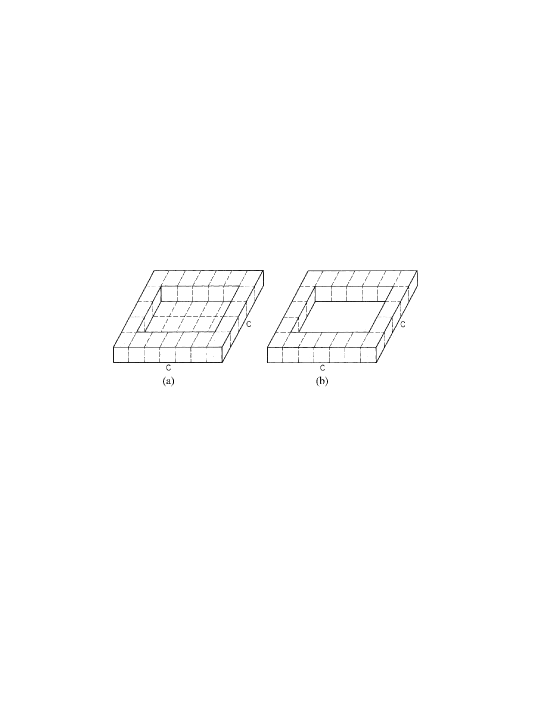
Figure 2: Strong-coupling diagrams that represent $N$-ality dependence: (a) area law and (b) perimeter law.

Main building block of three-dimensional diagram is Bianchi identity that lives on the cube. To reproduce the ”sandwich” type diagram one has to put $\lambda_{x}=0$ for all cubes except those which have a plaquette in common with the minimal surface bounded by the loop. For such cubes one should take $\lambda=j-1/2$. In the next plane we take $\lambda=j-1$ and so on. Combining this with fundamental plaquettes from the action results in the contribution of the form

$$\left[\frac{I_{2}(\beta)}{I_{1}(\beta)}\right]^{jA(C)}e^{-\widetilde{\mu}_{j}P(C)}+...\ .$$ (57)

At the invariant integration connectors are dropped out. It is easy to see the diagrams of this type could be constructed without connectors at all (i.e., with abelianized Bianchi identity) at least in the lowest order. So, in this case the contribution from connectors is trivial.

However, one cannot get the strong coupling diagram that represents $N$-ality dependence of the string tension without connectors. As example, consider the $j=1$ case. First, we construct ”tube” from cubes in the fundamental representation (see Fig.(2)) and cover all outer plaquettes by plaquettes taken from the action. Second, as is seen from formula (8) to get a nontrivial result of the invariant integration we need to cover all plaquettes from the surface by some plaquettes from additional Bianchi identities in the representation $j=1$. Third, if we omit connectors from all Bianchi identities we shall get a zero result due to integration over outer noncompensated plaquettes from these additional cubes. Clearly, it is impossible to build such ”tube” from plaquettes of abelianized Bianchi identity. A result of the invariant integration would give a vanishing contribution in this case. Thus, connectors appear to be a necessary element in constructing correct $N$-ality dependence.

References

• [1] J.ย Greensite, Prog.Part.Nucl.Phys. 51 (2003) 1.
• [2] A.M.ย Polyakov, Nucl.Phys.B 120 (1977), 429.
• [3] T.ย Banks, J.ย Kogut, R.ย Myerson, Nucl.Phys.B 121 (1977) 493.
• [4] M.ย Gรถpfert, G.ย Mack, Commun.Math.Phys. 82 (1982) 545.
• [5] A.ย Di Giacomo, Nucl.Phys.Proc.Suppl. 207-208 (2010) 337.
• [6] F.ย Conrady, Analytic derivation of dual gluons and monopoles from $SU(2)$ lattice Yang-Mills theory. III. Plaquette representation, 2006, arXiv:hep-th/0610238.
• [7] M.B.ย Halpern, Phys.Rev.D 19 (1979) 517; Phys.Lett. B 81 (1979) 245.
• [8] G.ย Batrouni, Nucl.Phys.B 208 (1982) 467.
• [9] O.ย Borisenko, S.ย Voloshin, M.ย Faber, Analytical study of low temperature phase of $3D$ LGT in the plaquette formulation, in Proc. of NATO Workshop โ€Confinement, Topology and Other Non-perturbative Aspects of QCDโ€ , Ed. by J.ย Greensite and ล .ย Olejnรญk, Kluwer Academic Publishers, 2002, 33.
• [10] O.ย Borisenko, S.ย Voloshin, M.ย Faber, Nucl. Phys. B 816 [FS] (2009) 399.
• [11] O.ย Borisenko, V.ย Kushnir, A.ย Velytsky, Phys.Rev. D 62 (2000) 025013.
• [12] A.M.ย Polyakov, Gauge Fields and Strings (Contemporary Concepts of Physics: v.3), Harwood Academic Publishers, Chur and London, 1987.
• [13] J.ย Ambjorn, J.ย Greensite, JHEP 9805 (1998) 004.