Statistical Analysis of an AGN sample with Simultaneous UV and X-ray Observations with Swift

Abstract:

I report on the statistical analysis of a sample of about 100 AGN with simultaneous UV and X-ray observations with Swift. I found clear correlations between the X-ray spectral slope $\alpha_{\rm X}$, the UV slope $\alpha_{\rm UV}$, and the optical-to-x-ray spectral slope $\alpha_{\rm ox}$with the Eddington ratio $L/L_{\rm Edd}$. I also report on the bolometric corrections for $L_{\rm 0.2-2.0keV}$ and $L_{5100\AA}$. A major aspect of the statistical analysis is multi-variate analysis statistical tools such as the Principal Component Analysis (PCA) and cluster analysis. This analysis shows that the main driver of the AGN properties in this sample is the Eddington ratio $L/L_{\rm Edd}$. Although separating Seyfert 1s into NLS1s and BLS1s is a good classification, with the 2000 km s^-1 cutoff line it is still arbitrary. A better classification scheme may be to separate AGN into low and high $L/L_{\rm Edd}$ AGN as suggested from the cluster analysis.

1 Introduction

After the milestone paper by [25] Narrow Line Seyfert 1 galaxies (NLS1s) have become an important part in AGN research. Their extreme properties place them at one end of the AGN population, often known as the eigenvector 1 relation in AGN (e.g. [2, 30, 14, 18]). This eigenvector 1 is typically associated with the Eddington ratio $L/L_{\rm Edd}$ which seem to drive the properties of AGN. $L/L_{\rm Edd}$ is therefore a crucial parameter to describe AGN. However, only for a small fraction of AGN it is possible to directly determine $L/L_{\rm Edd}$. For the majority of AGN we rely on secondary methods like a bolometric correction (e.g. [7, 32]) which calculate the bolometric luminosity based on the luminosity at the specific wavelength.

In these proceedings I discuss the bolometric correction based on simultaneous UV and X-ray observations obtained by Swift. This study was performed on a sample of 92 AGN [23] which will also show how spectral slope can be used as an estimator of $L/L_{\rm Edd}$. When [25] and [11] described NLS1s, they defined their definitions purely phenomenologically. After more than 25 years, is the definition of NLS1s just based on their FWHM(H$\beta$)$<$2000 km s^-1 still valid, or do we have to extend this definition? Here multi-variate analysis techniques come into play. With these techniques we can put the definition on a more solid statistical basis.

2 NLS1s in the Literature

When I gave a talk on NLS1 statistics at the 1999 Bad Honnef NLS1 meeting, I started out showing how NLS1s had become more and more popular over the previous decade and the number of publications with the word(s) ”NLS1” or ”Narrow-Line Seyfert 1” in their title had grown exponentially [15]. Are NLS1s still relevant in the literature today (March 2011) and more importantly, are NLS1s still an active research field? Figure 1 displays the numbers of papers per year have the name ”NLS1” or ”Narrow-Line Seyfert 1” in their title or abstract. The red triangles display the refereed publications and the blue circles show all publications. The number of NLS1 publications peaked at around 2001/2002, but still is at a level of roughly 100 publications per year including 50-60 refereed articles. Still, NLS1s are a very active field in the AGN community.

Another support for this statement is that at the 1999 Bad Honnef NLS1 meeting we had 60 participants. Of these only 6 are at this 2011 meeting in Milan which has more than 80 participants. So, in other words, NLS1s have attracted a lot of new people in the field. As shown in the articles in these proceedings, the field of NLS1s has really developed dramatically over the past ten years and we do have a much better understanding now in 2011 what the place of NLS1s in the Universe is than we had in 1999.

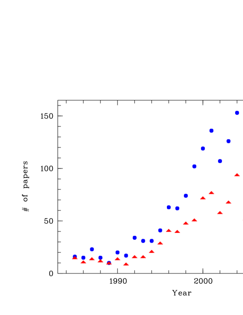
Figure 1: Papers per year which have the name ”NLS1” or ”Narrow-Line Seyfert 1” in their title or abstract. The red triangles display the refereed publications and the blue circles show all publications.

3 Sample Selection

Our AGN sample is selected from the ROSAT bright soft X-ray AGN sample by [16, 17] which contains a total of 110 AGN. There are several advantages of this particular AGN sample. First, all AGN in the sample are not only X-ray bright, but they are also bright in the Optical/UV which allows us to obtain high quality data in a relatively short amount of observing time. All of the AGN are intrinsically unabsorbed in X-rays and do not show high reddening in the UV. By definition, all of these AGN have at least one ROSAT observation which allows studies of their long-term variability. We also obtained optical spectroscopy data for all AGN [17] which enable us to perform multi-variate statistical analysis between emission line and continuum properties.

Of the 110 AGN, 92 had been observed by Swift by January 2010 and the results of these observations were published in [23]. By Mid-2011 this sample has been observed almost entirely. Half of the AGN in the sample are NLS1. Almost all of the AGN have been observed in Swift’s UV/Optical telescope (UVOT; [27]) in all 6 filters, which allows us to determine the Optical/UV slope $\alpha_{\rm UV}$ and the majority of the AGN has been visited by Swift multiple times, which gives us a handle on the variability in these sources. Many of these AGN show very strong variability in X-rays as well as in the UV [23], which makes it necessary to observe the Optical/UV and X-ray bands simultaneously when studying the spectral energy distributions of AGN. The data analysis of the Swift observations of the AGN in the sample is described in [23].

4 Swift

The Swift Gamma-Ray Burst observatory was launched in November 2004 [10]. While its prime objective was to detect and follow up on Gamma-Ray bursts, Swift has turned into a multi-purpose observatory due to its fast slewing and response capacity and its multi-wavelength coverage. As shown in Figure 2, Swift is equipped with three telescopes, the Burst Alert Telescope (BAT; [1]) which covers the 15-150 keV range, the X-ray telescope (XRT; [5]) covering the 0.3-10 keV energy band, and the UV/Optical Telescope (UVOT; [27]) covering the 1800-6000Å wavelength range. The simultaneous X-ray and UV coverage makes Swift and ideal observatory for AGN.

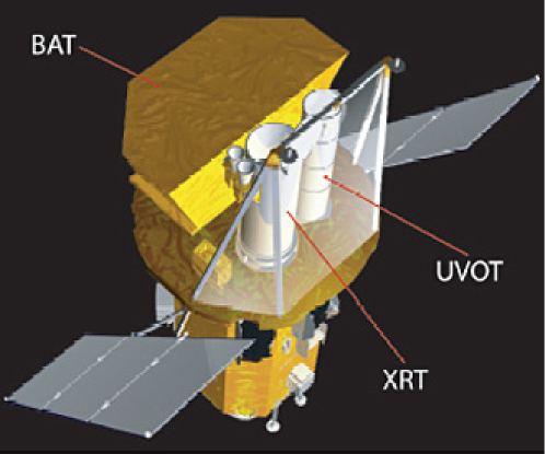
Figure 2: The Swift Gamma-Ray Burst Explorer Mission is equipped with the BAT, XRT and UVOT. (Credit: NASA/GSFC)

5 Simple correlation analysis

The full simple statistical analysis of the Swift AGN sample can be found in [23]. In these proceedings we only show a few of the correlations found among the sample.

As mentioned in the introduction, one way to determine the bolometric luminosity and therefore $L/L_{\rm Edd}$ is through bolometric corrections. From our sample we found the following bolometric corrections for the luminosity at 5100Å and the rest-frame 0.2-2.0 keV band:

$$\log L_{\rm bol}~{}=~{}(1.32\pm 0.06)\times\log L_{\rm 5100}~{}-~{}(10.84\pm 2.21).$$ (1)

$$\log L_{\rm bol}~{}=~{}(1.23\pm 0.06)\times\log L_{\rm X}~{}-~{}(7.36\pm 2.01).$$ (2)

These relations are displayed in Figure 17 in [23].

In particular we were interested in relations between $L/L_{\rm Edd}$ and spectral slopes. Figure 3 displays the relation between the X-ray spectral slope and $L/L_{\rm Edd}$. This is a strong correlation which is actually dominated by the Broad Line Seyfert 1. NLS1s with the $L/L_{\rm Edd}$ at unity do not show a dependence of the X-ray spectral slope with $L/L_{\rm Edd}$. The relation between $L/L_{\rm Edd}$ and $\alpha_{\rm X}$ found among the Swift AGN sample confirms earlier results by [17] using ROSAT results and [29] using the 2-10 keV spectral slopes that high $L/L_{\rm Edd}$ AGN have steeper X-ray continua than low $L/L_{\rm Edd}$ AGN.

Figure 4 shows the anti-correlation between $L/L_{\rm Edd}$ and the Optical/UV spectral slope $\alpha_{\rm UV}$. AGN with higher $L/L_{\rm Edd}$ display bluer optical/UV spectra. Note that there is an offset between NLS1s and BLS1s with NLS1s showing higher Eddington ratio for a given UV spectral slope than BLS1s [23]. We also notices a strong correlation between $L/L_{\rm Edd}$ and the optical to X-ray spectral slope $\alpha_{\rm ox}$ as shown in Figure 5. AGN with higher $L/L_{\rm Edd}$ appear to be X-ray weaker [23].

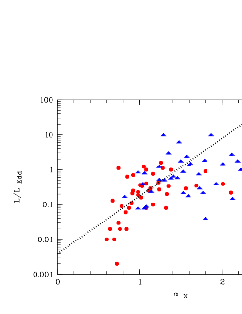
Figure 3: Correlations between the Eddington ratio $L/L_{\rm Edd}$ and the X-ray spectral slope $\alpha_{\rm X}$. NLS1 are displayed as blue triangles and BLS1s as red squares.

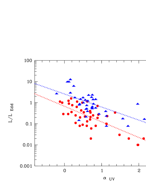
Figure 4: Correlations between the Eddington ratio $L/L_{\rm Edd}$ and the Optical/UV spectral slope $\alpha_{\rm UV}$. NLS1 are displayed as blue triangles and BLS1s as red squares.

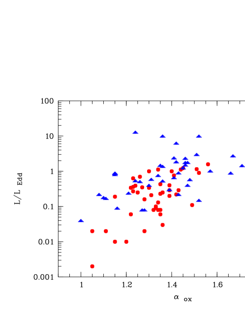
Figure 5: Correlations between the Eddington ratio $L/L_{\rm Edd}$ and optical to X-ray spectral slope $\alpha_{\rm ox}$. NLS1 are displayed as blue triangles and BLS1s as red squares.

6 Multi-variate Analysis

Instead of only looking for linear relations between measured parameters in a sample, multi-variate analysis examines the full data set in multiple dimensions. Multi-variate analysis looks into the n-dimensional parameter space and is searching for underlying properties/components that drives the observed parameters. It also searches for groups/clusters in this parameter space and by inter-weaving the different methods is able to find new relations and classes within the data set.

6.1 Statistical software R

All of the multi-component statistical analysis methods shown here used the statistical package R (e.g. [8, 28]). R is an object-oriented language for statistical data analysis. It is an extremely powerful package and unlike commercial statistical software packages, R is a free package that is continuously maintained and developed . R provides a huge library of statistical analysis packages that can be used for astronomical purposes.

6.2 Principle Component Analysis

The Principal Component Analysis (PCA) is a relatively old statistical tool, already developed more than 100 years ago (Pearson 1901). The idea of the PCA is to reduce the number of parameters in a sample to a small number of significant parameters that capture most of the variance in the data. For example when we look at the parameters that can be measured from stars they can basically be described by their mass and metallicity. In a mathematical sense, the PCA searches for the eigenvalues and eigenvectors in a correlation coefficient matrix:

$$A\times x=\lambda\times x$$ (3)

where $A$ is the correlation coefficient matrix, $\lambda$ an eigenvalue and $x$ an eigenvector. In a geometrical sense, the PCA performs an axis transformation for the cloud of data points in this n-dimensional space (n input parameters/properties). The first principal component is the eigenvector which direction is along the longest elongation of this cloud. The second eigenvector is the vector perpendicular this this one in the direction of the second largest elongation of the data cloud, and so forth. A good description for the application of a PCA in astronomy can be found in [9, 2]. Always keep in mind that a PCA is a purely mathematical method that can but does not necessarily result in physically meaningful parameters.

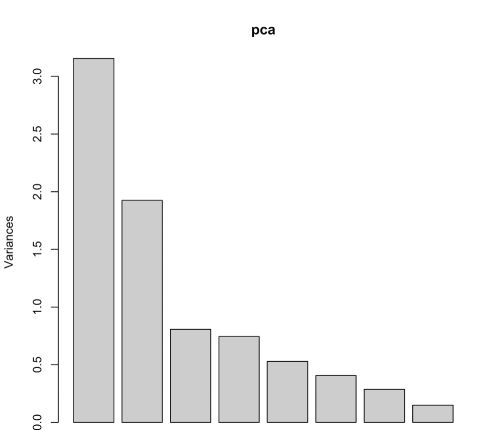
Figure 6: Strength of the eigenvectors from the Principal Component Analysis of our AGN sample. The columns represent each eigenvector starting with eigenvector 1 at the left.

When applying the PCA to the AGN sample by using $\alpha_{\rm X}$, $\alpha_{\rm UV}$, $\alpha_{\rm ox}$, FWHM(H$\beta$), FWHM([OIII]), [OIII]/H$\beta$, FeII/H$\beta$, and $L_{\rm 0.2-2.0keV}$ as input parameters we found that the first two eigenvectors already account for 64% of the variance in the sample. Figure 6 displays the strengths of the eigenvectors. A stronger eigenvector 1 results is steeper X-ray spectra, bluer optical spectra, steeper $\alpha_{\rm ox}$. We also found the well-known eigenvector 1 [OIII] and FeII Boroson & Green [2] relation. These relations suggests that eigenvector 1 is associated with $L/L_{\rm Edd}$. Figure 7 displays the relation between eigenvector 1 and $L/L_{\rm Edd}$ and indeed it shows there is a very strong correlation between these two properties. Looking at eigenvector 2, we interpret this eigenvector with the mass of the central black hole.

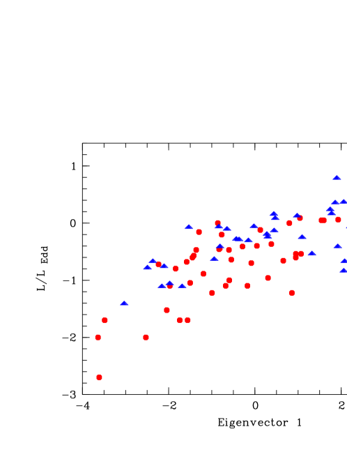
Figure 7: Eigenvector 1 vs. $L/L_{\rm Edd}$, again NLS1s are displayed as blue triangles and BLS1s as red squares.

6.3 Cluster Analysis

Figure 8: Dendrogram of the hierarchical cluster analysis of the AGN sample. Clearly the AGN sample can be divided into two groups.

The other multi-component technique is cluster analysis. Cluster analysis is a purely statistical/mathematical tool that allows an unbiased search for groups in multi-dimensional data sets. In its simplest form, the cluster analysis will search for the nearest neighbor in the parameter space. It will then group these neighbors with other groups of neighbors and so on. This is also called hierarchical clustering (e.g. [6]). At the end we will get a so called dendrogram such as displays for our AGN sample in Figure 8. Clustering is a powerful tool for data mining. It can and will find groups and correlations that are otherwise missed with simple analysis and classifications tools. A consistency-check of the results of the cluster analysis can be done again through the PCA. The groups found in the cluster analysis should also be found as groups in the eigenvector 1 - eigenvector 2 diagram from a PCA.

Figure 8 displays the dendrogram for our AGN sample using the sample input parameters as used for the PCA. Clearly the AGN can be separated into two classes. By itself, cluster analysis is a purely mathematical method and these groups may not mean anything. However, let’s have a look what the properties of the two groups are. Group 1 shows steeper X-ray spectra, bluer optical/UV continua and steeper optical to X-ray spectral slopes $\alpha_{\rm ox}$. It also contains mostly objects with narrower H$\beta$ lines and higher $L/L_{\rm Edd}$ Eddington ratios. The AGN in group 1 are those with the strongest FeII and weakest [OIII] emission. Does this mean that group 1 contains mostly NLS1s and group 2 BLS1s? Let’s have at first a look at the eigenvector 1 and eigenvector 2 diagram as we found it from the PCA. This graph is shown in Figure 9. The members of group 1 in this plot are shown as (blue) triangles. These are the objects with high eigenvector 1s and as we have seen before in the PCA, these are the objects with high $L/L_{\rm Edd}$. While 62% of the members in group 1 are NLS1s, only 20% of the members of group 2 are NLS1s, which is more the typical fraction of NLS1s found among AGN.

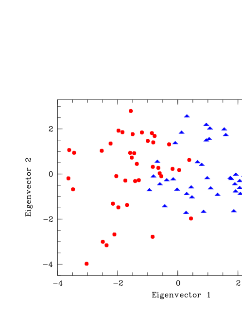
Figure 9: Eigenvector 1 vs. eigenvector 2 from the PCA using the two main groups found by the cluster analysis. Group 1 is displayed as blue triangles and group 2 as red squares.

Finally we can ask if the cutoff line between NLS1s and BLS1s at 2000 km s^-1 is still a valid definition. The answer is yes and no. No, because the 2000 km s^-1 definition is purely arbitrary and there are many sources with NLS1-like properties, but which do have broader FWHM(H$\beta$) than the 2000 km s^-1 definition. Yes, because a majority of NLS1s fall into our group 1. All in all, NLS1 is still a valid class/definition, but we should be more flexible about the cutoff line. We should generally speaking talk more about high $L/L_{\rm Edd}$ AGN because this definition is based on a more statistical and physical definition.

7 Discussion and Conclusions

Although NLS1 research is now more than 25 years old, it is still an active field in AGN research with still creates a lot of interest. It remains to be a powerful research area which generates more than 50 refereed publications each year. To make it clear, NLS1s are not an historical accident! NLS1s are extreme AGN, but they are needed for our interpretation of the AGN phenomenon.

Extending our statistical study into n-dimensional parameter space by using multi-variate tools like the PCA and cluster analysis shows that AGN separate into high and low $L/L_{\rm Edd}$ objects. The high $L/L_{\rm Edd}$ sample is mostly represented by NLS1s. Although the 2000 km s^-1 cutoff line between NSL1s and BLS1s is somewhat arbitrary, NLS1 still remains to be a valid AGN class.

- [1] S.D. Barthelmy, 2005, Space Science Reviews, 120, 143
- [2] T.A. Boroson, & R.F. Green, 1992, ApJS, 80, 109
- [3] T.A. Boroson, 2002, ApJ, 565, 78
- [4] W.N. Brandt, & S.C. Gallagher, 2000, New Astronomy Review, 44, 461
- [5] D.N. Burrows, et al., 2005, Space Science Reviews, 120, 165
- [6] R.O Duda, P.E. Hart, & D.G Stork, 2001, Pattern Classification, Wiley & Sons
- [7] M. Elvis, et al., 1994, ApJS, 95, 1
- [8] M.J Crawley, 2007, The R Book, Wiley & Sons
- [9] P.J. Francis, & B.J. Wills, 1999, ASP Conf. Series, 162, 363
- [10] N. Gehrels, et al., 2004, ApJ, 611, 1005
- [11] R.W. Goodrich, 1989, ApJ, 342, 224
- [12] R.W. Goodrich, 2000, New Astronomy Review, 44, 519
- [13] D. Grupe, et al., 1995, A&A, 300, L21
- [14] D. Grupe, K. Beuermann, K. Mannheim, & H.-V. Thomas, 1999, A&A, 350, 805
- [15] D. Grupe, 2000, New Astronomy Review, 44, 455
- [16] D. Grupe, H.-C. Thomas, & K. Beuermann, K., 2001, A&A, 367, 470
- [17] D. Grupe,B.J. Wills, K.M. Leighly, & H. Meusinger, 2004a, AJ, 127, 156
- [18] D. Grupe, 2004, AJ, 127, 1799
- [19] D. Grupe, et al., 2007a, AJ, 133, 1988
- [20] D. Grupe, S. Komossa, & L.C. Gallo, 2007b, ApJ, 681, 982
- [21] D. Grupe, et al., 2008a, ApJ, 681, 982
- [22] D. Grupe, K.M. Leighly, & S. Komossa, 2008b, AJ, 136, 2343
- [23] D. Grupe, S. Komossa, K.M. Leighly, & K.L. Page, 2010, ApJS, 187, 64
- [24] K.M. Leighly, F. Hamann, D.A. Casebeer, & D. Grupe, 2009, ApJ, 701, 176
- [25] D.E. Osterbrock & R.W. Pogge, 1985, ApJ, 297, 166
- [26] K. Pearson, 1901, Philosophical Magazine 2, 559
- [27] P.W.A. Roming, et al., 2005, Space Science Reviews, 120, 95
- [28] R Development Core Team (2009). R: A language and environment for statistical computing. R Foundation for Statistical Computing, Vienna, Austria. ISBN 3-900051-07-0, URL http://www.R-project.org.
- [29] O. Shemmer, W.N. Brandt, H. Netzer, R. Maiolino, & S. Kaspi, 2008, ApJ, 682, 81
- [30] J.W. Sulentic, T. Zwitter, P Marziani, & D. Dultzin-Hacyan, 2000, ApJ, 536, L5
- [31] H. Tananbaum, et al., 1979, ApJ, 234, L9
- [32] R.V. Vasudevan, & A.C. Fabian, 2009, MNRAS, 392, 1124