Poisson Yang-Baxter maps with binomial Lax matrices

Abstract

A construction of multidimensional parametric Yang-Baxter maps is presented. The corresponding Lax matrices are the symplectic leaves of first degree matrix polynomials equipped with the Sklyanin bracket. These maps are symplectic with respect to the reduced symplectic structure on these leaves and provide examples of integrable mappings. An interesting family of quadrirational symplectic YB maps on $\mathbb{C}^{4}\times\mathbb{C}^{4}$ with $3\times 3$ Lax matrices is also presented.

1 Introduction

Set theoretical solutions of the quantum Yang-Baxter equation have extensively been studied by many authors after the pioneer work of Drinfeld [5]. Even before that, examples of such solutions appeared in [20] by Sklyanin. Weinstein and Xu [24] proposed a construction of such solutions using the dressing action of Poisson Lie groups [18]. This was generalized later in [11], in order to construct solutions on any group that acts on itself and the action satisfies a compatibility condition. The algebraic aspects of the Yang-Baxter equation were developed by Etingof, Schedler and Soloviev [6].

Veselov [22, 23] connected the set theoretical solutions of the quantum Yang-Baxter equations with integrable mappings. More specifically, he proved that for such a solution, that admits a Lax matrix, there is a hierarchy of commuting transfer maps which preserve the spectrum of the corresponding monodromy matrix. Furthermore he proposed the shorter term ‘Yang Baxter maps’ for the set theoretical solutions of the quantum Yang-Baxter equation.

Yang-Baxter maps are closely related with integrable equations on quad-graphs. This is due to the multidimensional consistency property of these equations, introduced in [4, 12], which in a way seems to be equivalent with the Yang-Baxter property. An explicit classification of equations on quad-graphs with fields in $\mathbb{C}$ that satisfy the 3-dimensional consistency property and of the Yang-Baxter maps on $\mathbb{CP}^{1}\times\mathbb{CP}^{1}$ is given in [1] and [2] respectively (see also [14]). Higher dimensional Yang-Baxter maps are obtained from multi-field integrable lattice equations through symmetry reduction [15, 16].

Loop groups equipped with the Sklyanin bracket provide a natural framework in order to derive Yang-Baxter maps with polynomial Lax matrices. In [17] one of the most fundamental examples of a parametric Yang-Baxter map, Adler’s map, is given by Hamiltonian reduction of the loop group $LGL_{2}(\mathbb{R})$. Based on these ideas, a construction of Poisson parametric Yang-Baxter maps with first degree polynomial $2\times 2$ Lax matrices was presented by the authors [9] from a re-factorization procedure guided by the conservation of the Casimir functions under the maps. By considering a complete set of Casimir functions, symplectic multi parametric Yang-Baxter maps were derived with explicit formulae in terms of matrix operations.

The purpose of this work is to generalize the method of [9] in order to derive symplectic Yang-Baxter maps with Lax matrices that are obtained by reduction on symplectic leaves of binomial matrices.

The necessary definitions and notation about YB maps and Lax matrices, are given in section 2. Section 3 contains the main theory of the construction of symplectic Yang-Baxter maps associated to $2\times 2$ Lax matrices. This is generalized in higher dimensions in section 4 using further assumptions. A general re-factorization formula of $n\times n$ binomial matrices is presented. A reduction procedure of $3\times 3$ binomial matrices to four dimensional symplectic leaves, provides a family of quadrirational, symplectic YB maps on $\mathbb{C}^{4}\times\mathbb{C}^{4}$. Finally we conclude in section 5 by giving some comments and perspectives for future work.

2 Yang-Baxter Maps and lax matrices

Let $\mathcal{X}$ be any set. A map $R:\mathcal{X}\times\mathcal{X}\rightarrow\mathcal{X}\times\mathcal{X}$, $R:(x,y)\mapsto(u(x,y),v(x,y))$, that satisfies the Yang-Baxter equation :

$$R_{23}R_{13}R_{12}=R_{12}R_{13}R_{23}$$ (1)

is called Yang-Baxter Map (YB) [22]. Here by $R_{ij}$ for $i,j=1,...,3$, we denote the map that acts as $R$ on the $i$ and $j$ factor of $\mathcal{X}\times\mathcal{X}\times\mathcal{X}$ and identically on the others i.e.

$$R_{12}(x,y,z) = (u(x,y),v(x,y),z),$$

$$R_{13}(x,y,z) = (u(x,z),y,v(x,z)),$$

$$R_{23}(x,y,z) = (x,u(y,z),v(y,z)),$$

for $x,\ y,\ z\in\mathcal{X}$. From our point of view, we consider that the set $\mathcal{X}$ has the structure of an algebraic variety. The YB map $R$ is called non-degenerate if the maps $u(\cdot,y):\mathcal{X}\rightarrow\mathcal{X}$ and $v(x,\cdot):\mathcal{X}\rightarrow\mathcal{X}$ are bijective maps and quadrirational [2] if they are rational bijective maps.

Parametric YB maps appear in the study of integrable equations on quad-graphs. A parametric YB map is a YB map:

$$R:((x,\alpha),(y,\beta))\mapsto((u,\alpha),(v,\beta))=((u(x,\alpha,y,\beta),\alpha),(v(x,\alpha,y,\beta),\beta))$$ (2)

where $x,\ y\in\mathcal{X}$ and the parameters $\alpha,\beta\in\mathbb{C}^{n}$. We usually keep the parameters separately and denote $R(x,\alpha,y,\beta)$ by $R_{\alpha,\beta}(x,y)$. According to [21] a Lax Matrix for the YB map (2) is a matrix $L(x,\alpha,\zeta)$ that depends on the point $x$, the parameter $\alpha$ and a spectral parameter $\zeta$ (we usually denote it just by $L(x;\alpha)$), such that

$$L(u;\alpha)L(v;\beta)=L(y;\beta)L(x;\alpha),$$ (3)

for any $\zeta\in\mathbb{C}$. Furthermore if equation (3) is equivalent to $(u,\ v)=R_{\alpha,\beta}(x,y)$ then we will call $L(x;\alpha)$ strong Lax matrix.

A parametric YB map can be represented as a map assigned to the edges of an elementary quadrilateral like in Fig.1.

0.12 0.01 (7 1) 0.03 t:F (1 7) ( ) (0 0) 0.05 (8 0) (8 8) (0 8) (0 0) ( ) (2.8 -1.9)$(x;\alpha)$ (8.75 3.5)$(y;\beta)$ (2.8 8.5)$(u;\alpha)$ (-3.5 3.5)$(v;\beta)$ (4.3 3.8)$R_{\alpha,\beta}$

Figure 1: A map assigned to the edges of a quadrilateral

We can also represent the maps $R_{23}R_{13}R_{12}$ and $R_{12}R_{13}R_{23}$ as chains of maps at the faces of a cube like in Fig.2. The first map corresponds to the composition of the down, back, left faces, while the second one to the right, front and upper faces. All the parallel edges to the $x$ (resp. $y,z$) axis carry the parameter $\alpha$ (resp. $\beta$, $\gamma$). If we denote by $(x^{\prime\prime},y^{\prime\prime},z^{\prime\prime})$ and by $(\tilde{\tilde{x}},\tilde{\tilde{y}},\tilde{\tilde{z}})$ the corresponding values $R_{23}R_{13}R_{12}(x,y,z)$ and $R_{12}R_{13}R_{23}(x,y,z)$, then Eq.(1) assures that $x^{\prime\prime}=\tilde{\tilde{x}},\ y^{\prime\prime}=\tilde{\tilde{y}}$ and $z^{\prime\prime}=\tilde{\tilde{z}}$.

1.11 0.06

l:0.1 w:0.05

(1. 0) 0.01 (0.5 -0.5) () (0.5 0.5)() (1.0 1.0) () (0.5 0.5) ()(-0.5 0.5)() (0.0 1.0)(0.05 0.05)

(-2.5 0.0) (0.05 0.05) (-3.0 -0.5) () (-2.0 -0.5) () (-1.5 0.0) (0.05 0.05) (-2.5 -0.0) () (-1.5 0.0) (-1.5 1.0)() (-2.5 1.0) (0.05 0.05) (-2.5 0.0) () (-3.0 -0.5) (-3.0 0.5) ()

(-2.5 1.0) () (0 1) (1 1) ()(1 0)() (-0.5 0.5) (-0.5 -0.5) () (0.5 -0.5)()

(-2.6 0.1) (-2.9 0.5)() (-1.7 0.2) (-2.3 0.8)() (-2.1 -0.4) (-2.45 -0.1)() t:F (0.9 0.1) (0.6 0.5)() (0.3 -0.3) (-0.3 0.3)() (0.4 0.6) (0.05 0.9)()

(-0.05 -0.65) $x$ (0.8 -0.35) $y$ (1.05 0.45) $z$ (0.35 -0.05) $\tilde{z}$ (0.75 0.6) $\tilde{y}$ (-0.05 0.35) $\tilde{x}$ (-0.6 -0.05) $\tilde{\tilde{z}}$ (-0.4 0.7) $\tilde{\tilde{y}}$ (0.4 1.05) $\tilde{\tilde{x}}$

(-2.5 -0.65) $x$ (-1.7 -0.35) $y$ (-1.45 0.45) $z$ (-2.0 0.05) $x^{\prime}$ (-2.81 -0.22) $y^{\prime}$ (-2.0 1.05) $x^{\prime\prime}$ (-2.45 0.45) $z^{\prime}$ (-2.91 0.75) $y^{\prime\prime}$ (-3.18 -0.05) $z^{\prime\prime}$

(0.6 0.05) $R_{23}$ (-0.2 -0.2) $R_{13}$ (0.0 0.6) $R_{12}$

(-2.5 -0.4) $R_{12}$ (-2.2 0.3) $R_{13}$ (-2.9 0.05) $R_{23}$

(-3.2 -0.95) $(i)\ \ \ R_{23}R_{13}R_{12}$ (-0.7 -0.95) $(ii)\ \ \ R_{12}R_{13}R_{23}$

Figure 2: Cubic representation of the Yang–Baxter property

The following proposition [22, 9] gives a sufficient condition for a solution of the Lax equation (3), in order to satisfy the Yang-Baxter property.

Proposition 2.1.

Let $u=u_{\alpha,\beta}(x,y)$, $v=v_{\alpha,\beta}(x,y)$ and $A(x;\alpha)$ a matrix depending on a point $x$, a parameter $\alpha$ and a spectral parameter $\zeta$, such that $A(u;\alpha)A(v;\beta)=A(y;\beta)A(x;\alpha)$. If the equation

$$A(\hat{x};\alpha)A(\hat{y};\beta)A(\hat{z};\gamma)=A(x;\alpha)A(y;\beta)A(z;\gamma)$$ (4)

implies that $\hat{x}=x,\ \hat{y}=y$ and $\hat{z}=z$, then the map $R_{\alpha,\beta}(x,y)=(u,v)$ is a parametric Yang-Baxter map with Lax matrix $A(x;\alpha)$.

In a more general setting concerning integrable lattices (not necessary YB maps), instead of the notion of a Lax matrix, the notion of a Lax pair is more suitable. A Lax pair for a map $\Phi_{\alpha,\beta}:((x,\alpha),(y,\beta))\mapsto((u,\alpha),(v,\beta))=((u(x,\alpha,y,\beta),\alpha),(v(x,\alpha,y,\beta),\beta))$ is a pair of matrices $L,\ M$ depending on a point in $\mathcal{X}$, a parameter and a spectral parameter $\zeta$ such that

$$L(u,\alpha,\zeta)M(v,\beta,\zeta)=M(y,\beta,\zeta)L(x,\alpha,\zeta),$$ (5)

for any $\zeta\in\mathbb{C}$. Combinations of Lax pairs can provide solutions of the entwining Yang-Baxter equation [10].

The dynamical aspects of the Yang-Baxter maps have been extensively investigated in [22] and [23] where commuting transfer maps, that preserve the spectrum of the corresponding monodromy matrices, are introduced for each YB map. These maps are believed to be integrable in the Liouville sense, i.e. symplectic mappings $M^{2n}\rightarrow M^{2n}$ that admit $n$ functionally independent integrals in involution.

3 Symplectic Yang–Baxter maps associated to binomial $2\times 2$ Lax matrices

A general matrix re-factorization procedure provides a way of constructing rational multi-parametric Yang-Baxter maps on $\mathbb{C}^{4}\times\mathbb{C}^{4}$ with $2\times 2$ Lax matrices in the form of first-degree matrix polynomials. These maps are Poisson with respect to the Sklyanin bracket. By reduction on symplectic leaves we derive 4-dimensional symplectic parametric YB maps. The whole procedure generalizes the one presented in [9], where the leading terms of the matrix polynomials were assumed equal.

3.1 Poisson Yang–Baxter maps from matrix re-factorization

We consider the set $\mathcal{L}^{2}$ of $2\times 2$ polynomial matrices of the form $L(\zeta)=X-\zeta A$, $\zeta\in\mathbb{C}$ equipped with the Sklyanin bracket [19]:

$$\{L(\zeta)\ \overset{\otimes}{,}\ L(\eta)\}=[\frac{r}{\zeta-\eta},L(\zeta)\otimes L(\eta)],$$ (6)

where $r$ denotes the permutation matrix: $r(x\otimes y)=y\otimes x$. For

$$X=\begin{pmatrix}x_{1}&x_{2}\\ x_{3}&x_{4}\end{pmatrix}\ {\text{and}}\ \ A=\begin{pmatrix}a_{1}&a_{2}\\ a_{3}&a_{4}\end{pmatrix},$$

the brackets between the coordinate functions are given by the antisymmetric Poisson structure matrix :

$$J_{A}(X)=\begin{pmatrix}0&-x_{2}a_{1}+x_{1}a_{2}&x_{3}a_{1}-x_{1}a_{3}&x_{3}a_{2}-x_{2}a_{3}\\ *&0&x_{4}a_{1}-x_{1}a_{4}&x_{4}a_{2}-x_{2}a_{4}\\ *&*&0&-x_{4}a_{3}+x_{3}a_{4}\\ *&*&*&0\end{pmatrix}$$ (7)

where $J_{A}(X)_{ij}=\{x_{i}-\zeta a_{i},x_{j}-\zeta a_{j}\}$, for $i,j=1,...,4$.

There are six linear independent Casimir functions of $\mathcal{L}^{2}$ which are the elements $a_{i}$, $i=1,...,4$, of the matrix $A$ and the functions:

$$f_{0}(X;A)=\det X,\ \ f_{1}(X;A)=a_{4}x_{1}-a_{3}x_{2}-a_{2}x_{3}+a_{1}x_{4},$$

i.e. the coefficients of the polynomial

$$p_{X}^{A}(\zeta):=\det(X-\zeta A)=f_{2}(X;A)\zeta^{2}-f_{1}(X;A)\zeta+f_{0}(X;A)$$

with $f_{2}(X;A)=\det A$ (of course $f_{2}(X;A)$ is also Casimir). For any constant matrix $A$ we denote by $i_{A}$ the immersion $i_{A}:X\mapsto X-\zeta A$ and by $\mathcal{L}^{2}_{A}$ the level set

$$\mathcal{L}^{2}_{A}=\{X-\zeta A\ |\ X\in Mat(2\times 2)\}.$$

Furthermore for any pair of matrices $A,~{}B\in GL_{2}(\mathbb{C})$, we define the matrix functions $\Pi_{A,B}^{1},\ \Pi_{A,B}^{2},$ with

$$\Pi^{1}_{A,B}(X,Y) = f_{2}(X;A)(YA+BX)-f_{1}(X;A)AB,$$ (8)

$$\Pi^{2}_{A,B}(X,Y) = f_{2}(X;A)YX-f_{0}(X;A)AB.$$ (9)

Proposition 3.1.

(re-factorization) Let $A,\ B$ be invertible $2\times 2$ matrices, such that $AB=BA$ and $X,Y\in Mat(2\times 2)$ with $\det\Pi^{1}_{A,B}(X,Y)\neq 0$ . Then

$$(U-\zeta A)(V-\zeta B)=(Y-\zeta B)(X-\zeta A),$$ (10)

and $p_{U}^{A}(\zeta)=p_{X}^{A}(\zeta)$ (equivalently $p_{V}^{B}(\zeta)=p_{Y}^{B}(\zeta)$), iff

$$U=U_{A,B}(X,Y) := \Pi^{2}_{A,B}(X,Y)\Pi^{1}_{A,B}(X,Y)^{-1}A,$$ (11)

$$V=V_{A,B}(X,Y) := A^{-1}(YA+BX-U(X,Y)B).$$ (12)

The proof of this proposition is given in [10].

Lemma 1.

Let $A_{i},\ i=1,2,3$ be three invertible matrices such that $A_{i}A_{j}=A_{j}A_{i}$, for $i,j=1,2,3$. Then

$$(X^{\prime}_{1}-\zeta A_{1})(X^{\prime}_{2}-\zeta A_{2})(X^{\prime}_{3}-\zeta A_{3})=(X_{1}-\zeta A_{1})(X_{2}-\zeta A_{2})(X_{3}-\zeta A_{3})$$ (13)

and $p_{X^{\prime}_{i}}^{A_{i}}(\zeta)=p_{X_{i}}^{A_{i}}(\zeta)$ for every $X_{i}\in Mat(2\times 2),\ i=1,2,3$ and $\zeta\in\mathbb{C}$, iff $X^{\prime}_{1}=X_{1}$, $X^{\prime}_{2}=X_{2}$ $X^{\prime}_{3}=X_{3}$.

The proof of this lemma can be traced in the appendix of [10].

Proposition 3.2.

Let $K:\mathbb{C}^{d}\rightarrow GL_{2}(\mathbb{C})$, be a d–parametric family of commuting matrices. For every $\alpha,\beta\in\mathbb{C}^{d}$ the map

$$\mathcal{R}_{\alpha,\beta}(X,Y)=(U_{K(\alpha),K(\beta)}(X,Y),V_{K(\alpha),K(\beta)}(X,Y)):=(U,V)$$ (14)

defined by (11), (12), is a parametric Yang-Baxter map with Lax matrix $L(X;\alpha)=i_{K(\alpha)}(X)$ such that $p_{U}^{K(\alpha)}(\zeta)=p_{X}^{K(\alpha)}(\zeta)$ and $p_{V}^{K(\beta)}(\zeta)=p_{Y}^{K(\beta)}(\zeta)$.

Proof:

For $U=U_{K(\alpha),K(\beta)}(X,Y)$, $V=V_{K(\alpha),K(\beta)}(X,Y)$ and $L(X;\alpha)=i_{K(\alpha)}(X)$, from proposition 3.1 we have that

$$L(U;\alpha)L(V;\beta)=L(Y;\beta)L(X;\alpha)$$

and $p_{U}^{K(\alpha)}(\zeta)=p_{X}^{K(\alpha)}(\zeta)$, $p_{V}^{K(\beta)}(\zeta)=p_{Y}^{K(\beta)}(\zeta)$. Now, if we set

$$R_{\alpha,\beta}^{12}(X,Y,Z) = (X^{\prime},Y^{\prime},Z),$$

$$R_{\alpha,\gamma}^{13}\circ R_{\alpha,\beta}^{12}(X,Y,Z) = (X^{\prime\prime},Y^{\prime},Z^{\prime}),$$

$$R_{\beta,\gamma}^{23}\circ R_{\alpha,\gamma}^{13}\circ R_{\alpha,\beta}^{12}(X,Y,Z) = (X^{\prime\prime},Y^{\prime\prime},Z^{\prime\prime}),$$

then $L(Y;\beta)L(X;\alpha)=L(X^{\prime};\alpha)L(Y^{\prime};\beta)$, and $p_{X^{\prime}}^{K(\alpha)}(\zeta)=p_{X}^{K(\alpha)}(\zeta)$, $p_{Y^{\prime}}^{K(\beta)}(\zeta)=p_{Y}^{K(\beta)}(\zeta)$. So

$$L(Z;\gamma)L(Y;\beta)L(X;\alpha)=(L(Z;\gamma)L(X^{\prime};\alpha))L(Y^{\prime};\beta)=L(X^{\prime\prime};\alpha)(L(Z^{\prime};\gamma)L(Y^{\prime};\beta))$$

$$=L(X^{\prime\prime};\alpha)L(Y^{\prime\prime}\beta)L(Z^{\prime\prime};\gamma)\$$

$\text{and}\ p_{X^{\prime\prime}}^{K(\alpha)}(\zeta)=p_{X}^{K(\alpha)}(\zeta),\ p_{Y^{\prime\prime}}^{K(\beta)}(\zeta)=p_{Y}^{K(\beta)}(\zeta),\ p_{Z^{\prime\prime}}^{K(\gamma)}(\zeta)=p_{Z}^{K(\gamma)}(\zeta).$
On the other hand for

$$R_{\beta,\gamma}^{23}(X,Y,Z) = (X,\tilde{Y},\tilde{Z}),$$

$$R_{\alpha,\gamma}^{13}\circ R_{\beta,\gamma}^{23}(X,Y,Z) = (\tilde{X},\tilde{Y},\tilde{\tilde{Z}}),$$

$$R_{\alpha,\beta}^{12}\circ R_{\alpha,\gamma}^{13}\circ R_{\beta,\gamma}^{23}(X,Y,Z) = (\tilde{\tilde{X}},\tilde{\tilde{Y}},\tilde{\tilde{Z}})$$

we get $L(Z;\gamma)L(Y;\beta)L(X;\alpha)=L(\tilde{\tilde{X}};\alpha)L(\tilde{\tilde{Y}};\beta)L(\tilde{\tilde{Z}};\gamma)$ and $p_{\tilde{\tilde{X}}}^{K(\alpha)}(\zeta)=p_{X}^{K(\alpha)}(\zeta)$, $p_{\tilde{\tilde{Y}}}^{K(\beta)}(\zeta)=p_{Y}^{K(\beta)}(\zeta)$, $p_{\tilde{\tilde{Z}}}^{K(\gamma)}(\zeta)=p_{Z}^{K(\gamma)}(\zeta).$ So finally we have that

$$L(X^{\prime\prime};\alpha)L(Y^{\prime\prime}\beta)L(Z^{\prime\prime};\gamma) = L(\tilde{\tilde{X}};\alpha)L(\tilde{\tilde{Y}};\beta)L(\tilde{\tilde{Z}};\gamma),$$

$$p_{X^{\prime\prime}}^{K(\alpha)}(\zeta)~{}=~{}p_{\tilde{\tilde{X}}}^{K(\alpha)}(\zeta),\ p_{Y^{\prime\prime}}^{K(\beta)}(\zeta) = p_{\tilde{\tilde{Y}}}^{K(\beta)}(\zeta),\ p_{Z^{\prime\prime}}^{K(\gamma)}(\zeta)~{}=~{}p_{\tilde{\tilde{Z}}}^{K(\gamma)}(\zeta)$$

and from lemma 1 we derive $X^{\prime\prime}=\tilde{\tilde{X}},\ Y^{\prime\prime}=\tilde{\tilde{Y}},\ Z^{\prime\prime}=\tilde{\tilde{Z}}$, i.e.

$$R_{\beta,\gamma}^{23}\circ R_{\alpha,\gamma}^{13}\circ R_{\alpha,\beta}^{12}=R_{\alpha,\beta}^{12}\circ R_{\alpha,\gamma}^{13}\circ R_{\beta,\gamma}^{23}.$$

We will refer to the Yang-Baxter map of Prop. 3.2 as the general parametric Yang-Baxter map associated with the function $K$. We have to notice that in general the Lax matrix $L(X;\alpha)=i_{K(\alpha)}(X)$ is not a strong Lax matrix. For example by considering $K(\alpha)=B$ for a constant $B\in GL_{2}(\mathbb{C})$, the equation $i_{B}(U)i_{B}(V)=i_{B}(Y)i_{B}(X)$ except of the corresponding solution (11),(12), admits also the trivial solution $U=Y,\ V=X$ (elementary involution).

Now we return to the Poisson structure (7). We can extend the Poisson bracket of $\mathcal{L}^{2}$ to the Cartesian product $\mathcal{L}^{2}\times\mathcal{L}^{2}$ as follows :

$$\{x_{i},x_{j}\}=J_{A}(X)_{ij},\ \{y_{i},y_{j}\}=J_{B}(Y)_{ij},\ \{x_{i},y_{j}\}=0,$$ (15)

for any $(X-\zeta A,\ Y-\zeta B)\in\mathcal{L}^{2}\times\mathcal{L}^{2}$ where $x_{i},\ x_{j},\ y_{i},\ y_{j}$ for $i=1,...,4$ are the elements of the matrices $X,\ Y$ respectively.

Proposition 3.3.

The map $\mathcal{R}:\mathcal{L}^{2}_{K(\alpha)}\times\mathcal{L}^{2}_{K(\beta)}\rightarrow\mathcal{L}^{2}_{K(\alpha)}\times\mathcal{L}^{2}_{K(\beta)}$,

$$\mathcal{R}:(X-\zeta K(\alpha),Y-\zeta K(\beta))\mapsto(U_{K(\alpha),K(\beta)}(X,Y)-\zeta K(\alpha),V_{K(\alpha),K(\beta)}(X,Y)-\zeta K(\beta))$$ (16)

is a Poisson map.

Proof:

A direct computation of the Poisson brackets of the elements of $U=U_{K(\alpha),K(\beta)}(X,Y)$ and $V=V_{K(\alpha),K(\beta)}(X,Y)$ defined by (11), (12) gives:

$$\{u_{i},u_{j}\}=J_{K_{\alpha}}(U)_{ij},\ \{v_{i},v_{j}\}=J_{K_{\beta}}(V)_{ij},\ \{u_{i},v_{j}\}=0,$$

for $i=1,...,4$.

If we consider the permutation map $r:(X,Y)\mapsto(Y,X)$ and the multiplication map $m:(X,Y)\mapsto XY$, then $\mathcal{R}$ is the unique map defined by the commutative diagram:

$$Commutative\ diagram$$

Here $\mathcal{L}^{2}_{2}$ denotes the second degree polynomial $2\times 2$ matrices. From proposition 3.3 and the multiplication property of the Sklyanin bracket we conclude that each map of this diagram is Poisson.

3.2 Reduction on symplectic leaves

In the previous section it was pointed out that the matrix $A$ of a generic element

$$X-\zeta A=\begin{pmatrix}x_{1}&x_{2}\\ x_{3}&x_{4}\end{pmatrix}-\zeta\begin{pmatrix}a_{1}&a_{2}\\ a_{3}&a_{4}\end{pmatrix}\in\mathcal{L}^{2},$$

belongs to the center of the Sklyanin algebra. In the four dimensional Poisson submanifold $\mathcal{L}^{2}_{A}$ there are two Casimir functions

$$f_{0}(X;A)=\det X\ \text{ }\ \ f_{1}(X;A)=a_{4}x_{1}-a_{3}x_{2}-a_{2}x_{3}+a_{1}x_{4}.$$

We restrict on the level set of the Casimir functions by solving the system $f_{0}(X;{A})=\alpha_{0}$, $f_{1}(X;{A})=\alpha_{1}$ with respect to two elements $x_{i},x_{j}$ of $X$. So we consider two functions $h_{A},\ g_{A}$, defined on an open set $D\subset\mathbb{C}^{4}$, such that

$$x_{i}=h_{(}x_{k},x_{l},\alpha_{0},\alpha_{1})\ \text{and}\ x_{j}=g_{A}(x_{k},x_{l},\alpha_{0},\alpha_{1}),\ k,l\notin\{i,j\}.$$ (17)

We denote by $pr_{k,l}$ the projection of a matrix to its $k,l$ elements (by ordering the elements of a matrix from one to four as before) and by $Pr$ the map

$$Pr=pr_{k,l}\times pr_{k,l}:(X,Y)\mapsto(pr_{k,l}(X),pr_{k,l}(Y)).$$

By substituting the $x_{i},x_{j}$ to the matrix $X$ we define the parametric matrix $L^{\prime}_{A}(x_{k},x_{l};\alpha_{0},\alpha_{1})$. For simplicity we renumber $x_{k}\mapsto x_{1}$, $x_{l}\mapsto x_{2}$ and we come up to the matrix $L^{\prime}_{A}(x_{1},x_{2};\alpha_{0},\alpha_{1})$ that satisfies the following equations

$$f_{0}(L^{\prime}_{A}(x_{1},x_{2};\alpha_{0},\alpha_{1});A)=\alpha_{0}\ \text{ }\ f_{1}(L^{\prime}_{A}(x_{1},x_{2};\alpha_{0},\alpha_{1});A)=\alpha_{1}.$$

The connected components of $\Sigma_{A}(\alpha_{0},\alpha_{1})=\{L^{\prime}_{A}(x_{1},x_{2};\alpha_{0},\alpha_{1})-\zeta A\,|\ x_{1},x_{2}\in D\subset\mathbb{C}\}$ are two dimensional symplectic leaves of $\mathcal{L}^{2}_{A}$.

By the next proposition the general YB map $\mathcal{R}_{\alpha,\beta}$ of Prop. 3.2 is reduced on the symplectic leaves $\Sigma_{K(\alpha)}(\alpha_{0},\alpha_{1})\times\Sigma_{K(\beta)}(\beta_{0},\beta_{1})$ of $\mathcal{L}^{2}\times\mathcal{L}^{2}$.

Proposition 3.4.

Let $K:\mathbb{C}^{d}\mapsto GL_{2}(\mathbb{C})$ be a d–parametric family of commuting matrices. For every $\alpha,\beta\in\mathbb{C}^{d}$, the map

$$R_{\bar{\alpha},\bar{\beta}}((x_{1},x_{2}),(y_{1},y_{2}))=Pr\circ\mathcal{R}_{\alpha,\beta}(L^{\prime}_{K(\alpha)}(x_{1},x_{2};\alpha_{0},\alpha_{1}),L^{\prime}_{K(\beta)}(y_{1},y_{2};\beta_{0},\beta_{1})),$$ (18)

is a non-degenerate symplectic Yang-Baxter map with vector parameters $\bar{\alpha}=(\alpha,\alpha_{0},\alpha_{1})$, $\bar{\beta}=(\beta,\beta_{0},\beta_{1})\in V\times\mathbb{C}^{2}$ and strong Lax matrix

$$L(x_{1},x_{2};\bar{\alpha})=i_{K(\alpha)}(L^{\prime}_{K(\alpha)}(x_{1},x_{2};\alpha_{0},\alpha_{1}))=L^{\prime}_{K(\alpha)}(x_{1},x_{2};\alpha_{0},\alpha_{1})-\zeta K(\alpha).$$ (19)

Proof:

For $X=L^{\prime}_{K(\alpha)}(x_{1},x_{2};\alpha_{0},\alpha_{1})$ and $Y=L^{\prime}_{K(\beta)}(y_{1},y_{2};\beta_{0},\beta_{1})$ we define the matrices $U=U_{K(\alpha),K(\beta)}(X,Y),\ V=V_{K(\alpha),K(\beta)}(X,Y))$ by (11), (12)

$$(U,V)=\mathcal{R}_{\alpha,\beta}(X,Y)=\mathcal{R}_{\alpha,\beta}(L^{\prime}_{K(\alpha)}(x_{1},x_{2};\alpha,\alpha_{0},\alpha_{1}),L^{\prime}_{K(\beta)}(y_{1},y_{2};\beta,\beta_{0},\beta_{1})).$$

Since $f_{i}(U;K(\alpha))=f_{i}(X;K(\alpha))=\alpha_{i}$ and $f_{i}(V;K(\beta))=f_{i}(Y;K(\beta))=\beta_{i}$ for $i=0,1$, then $U=L^{\prime}_{K(\alpha)}(u_{1},u_{2};\alpha_{0},\alpha_{1})$ and $V=L^{\prime}_{K(\beta)}(v_{1},v_{2};\beta_{0},\beta_{1})$. The projection $Pr(U,V)$ gives the corresponding elements $u=(u_{1},u_{2})$ and $v=(v_{1},v_{2})$). So the YB property of the map $R_{\bar{\alpha},\bar{\beta}}:((x_{1},x_{2};\bar{\alpha}),(y_{1},y_{2};\bar{\beta}))\mapsto((u_{1},u_{2},\bar{\alpha}),(v_{1},v_{2},\bar{\beta}))$, is immediately derived from the YB property of the Poisson map $\mathcal{R}_{\alpha,\beta}$. Furthermore proposition 3.2 implies that $i_{K(\alpha)}(U)i_{K(\beta)}(V)=i_{K(\beta)}(Y)i_{K(\alpha)}(X)$, so

$$(L^{\prime}_{K(\alpha)}(u_{1},u_{2};\alpha_{0},\alpha_{1})-\zeta K_{\alpha})(L^{\prime}_{K(\beta)}(v_{1},v_{2};\beta_{0},\beta_{1})-\zeta K_{\beta})$$ (20)

$$= (L^{\prime}_{K(\beta)}(y_{1},y_{2};\beta_{0},\beta_{1})-\zeta K_{\beta})(L^{\prime}_{K(\alpha)}(x_{1},x_{2};\alpha_{0},\alpha_{1})-\zeta K_{\alpha})$$

which means that $L(x_{1},x_{2};\bar{\alpha})=L^{\prime}_{K(\alpha)}(x_{1},x_{2};\alpha_{0},\alpha_{1})-\zeta K_{\alpha}$ is a Lax matrix for $R_{\bar{\alpha},\bar{\beta}}$. Also, from proposition 3.1 we conclude that $L(x_{1},x_{2};\bar{\alpha})$ is a strong Lax matrix. Finally we notice that equation (20) is directly solvable with respect to $v=(v_{1},v_{2})$ and $x=(x_{1},x_{2})$, since

$$K_{\beta}^{-1}L^{\prime}_{K_{\beta}}(v;\hat{\beta})=(L^{\prime}_{K_{\alpha}}(u;\hat{\alpha})K_{\beta}-L^{\prime}_{K_{\beta}}(y;\hat{\beta})K_{\alpha})^{-1}L^{\prime}_{K_{\beta}}(y;\hat{\beta})K_{\beta}^{-1}(L^{\prime}_{K_{\alpha}}(u;\hat{\alpha})K_{\beta}-L^{\prime}_{K_{\beta}}(y;\hat{\beta})K_{\alpha}),~{}~{}$$

$$K_{\alpha}^{-1}L^{\prime}_{K_{\alpha}}(x;\hat{\alpha})=(L^{\prime}_{K_{\beta}}(y;\hat{\beta})K_{\alpha}-L^{\prime}_{K_{\alpha}}(u;\hat{\alpha})K_{\beta})^{-1}L^{\prime}_{K_{\alpha}}(u;\hat{\alpha})K_{\alpha}^{-1}(L^{\prime}_{K_{\beta}}(y;\hat{\beta})K_{\alpha}-L^{\prime}_{K_{\alpha}}(u;\hat{\alpha})K_{\beta})~{}~{}~{}$$

for $y=(y_{1},y_{2})$, $u=(u_{1},u_{2})$, $\hat{\alpha}=(\alpha_{0},\alpha_{1})$ and $\hat{\beta}=(\beta_{0},\beta_{1})$. That proves the non-degeneracy of the YB map (18).

Remark 3.5.

From the construction of the Lax matrix $L(x_{1},x_{2};\bar{\alpha})$ and lemma 1 we can prove that the equation:

$$L(x^{\prime}_{1},x^{\prime}_{2};\bar{\alpha})L(y^{\prime}_{1},y^{\prime}_{2};\bar{\beta})L(z^{\prime}_{1},z^{\prime}_{2};\bar{\gamma})=L(x_{1},x_{2};\bar{\alpha})L(y_{1},y_{2};\bar{\beta})L(z_{1},z_{2};\bar{\gamma})$$

implies $x^{\prime}=x,\ y^{\prime}=y$ and $z^{\prime}=z$ (without further assumptions). So the YB property of the map (18) can be derived directly from Prop. 2.1.

Remark 3.6.

If we set $\alpha_{0}=\beta_{0}=k$ on the YB map (18) we obtain the parametric YB map $R_{\bar{\alpha},\bar{\beta}}$ with parameters $\bar{\alpha}=(\alpha,a_{1}),\ \bar{\beta}=(\beta,b_{1})\in V\times\mathbb{C}$ and Lax matrix $L(x_{1},x_{2};\alpha,\alpha_{1}):=L(x_{1},x_{2};\alpha,k,\alpha_{1})$. We have analogous results if we identify any other pair of parameters. If we set $\bar{\alpha}=\bar{\beta}$ then we derive the trivial solution $U=Y$, $V=X$, because this is the only solution of Eq.(10) with $A=B$, $f_{0}(U;A)=f_{0}(Y;A)$ and $f_{1}(U;A)=f_{1}(Y;A)$.

3.3 Classification

In this section we classify the quadrirational YB maps with $2\times 2$ binomial Lax matrices of our construction. In [9] a classification by Jordan normal forms was given for the case $K(\alpha)=K(\beta)=B$, with $B$ a $2\times 2$ constant matrix. Here we give a more general classification in order to include all the cases that we considered. First we begin by determining the functions $K$ of proposition 3.2. Actually we are going to consider the problem of families of commuting matrices up to conjugation. One can bring one member of the family to its Jordan canonical form and find all matrices commuting with it. From this analysis we conclude that, up to conjugation, there are only two (non-disjoint) families of commuting pairs of matrices

$$I)\ A=\begin{pmatrix}a_{1}&0\\ 0&a_{2}\end{pmatrix},\ B=\begin{pmatrix}b_{1}&0\\ 0&b_{2}\end{pmatrix}\ \text{and}\ \ II)\ A=\begin{pmatrix}a_{1}&a_{2}\\ 0&a_{1}\end{pmatrix},\ B=\begin{pmatrix}b_{1}&b_{2}\\ 0&b_{1}\end{pmatrix}.$$

Since the equation (3) and the YB maps are invariant under conjugation we can restrict to these two general cases of the function $K:\mathbb{C}^{2}\rightarrow GL_{2}(\mathbb{C})$.

The last step towards the classification is to examine the relevance of the choice of variables in the construction of the Lax matrix that we presented in the previous section. In the first case, where $K(\alpha)$ is a matrix of the first family for any $\alpha\in\mathbb{C}^{2}$, the equations

$$f_{0}(X;K(\alpha))=\alpha_{0},\ f_{1}(X;K(\alpha))=\alpha_{1}$$ (21)

are solvable with respect to any pair $(x_{i},x_{j})$, for $i,j=1,...,4,\ i\neq j$, except of the pair $(x_{2},x_{3})$, while for a matrix $K(\alpha)$ of the second family the equations are solvable with respect to any pair $(x_{i},x_{j})$,$i,j=1,...,4,\ i\neq j$. Now, let us suppose that, by solving equations (21) in a different way, we have derived two matrices $L^{\prime}_{K(\alpha)}(x_{1},x_{2};\alpha_{0},\alpha_{1})$, $M^{\prime}_{K(\alpha)}(x^{\prime}_{1},x^{\prime}_{2};\alpha_{0},\alpha_{1})$ such that

$$f_{0}(L^{\prime}_{K(\alpha)}(x_{1},x_{2};\alpha_{0},\alpha_{1});K(\alpha)) = \alpha_{0},\ f_{1}(L^{\prime}_{K(\alpha)}(x_{1},x_{2};\alpha_{0},\alpha_{1});K(\alpha))=\alpha_{1}\ \text{and}\$$

$$f_{0}(M^{\prime}_{K(\alpha)}(x^{\prime}_{1},x^{\prime}_{2};\alpha_{0},\alpha_{1});K(\alpha)) = \alpha_{0},\ f_{1}(M^{\prime}_{K(\alpha)}(x^{\prime}_{1},x^{\prime}_{2};\alpha_{0},\alpha_{1}));K(\alpha))=\alpha_{1}.$$

Then there is a local diffeomorphism $\phi_{\bar{\alpha}}:\mathbb{C}^{2}\rightarrow\mathbb{C}^{2}$ ($\bar{\alpha}=(\alpha,\alpha_{0},\alpha_{1})\in\mathbb{C}^{4}$), such that $\phi_{\bar{\alpha}}:(x_{1},x_{2})\mapsto(x^{\prime}_{1},x^{\prime}_{2})$ and

$$M^{\prime}_{K(\alpha)}(\phi_{\bar{\alpha}}(x_{1},x_{1});\alpha_{0},\alpha_{1})=L^{\prime}_{K(\alpha)}(x_{1},x_{2};\alpha_{0},\alpha_{1}).$$

Now if we denote by $R_{\bar{\alpha},\bar{\beta}},\ R^{\prime}_{\bar{\alpha},\bar{\beta}}$ the parametric YB maps with strong Lax matrices $L(x_{1},x_{2};\bar{\alpha})=L^{\prime}_{K(\alpha)}(x_{1},x_{2};\alpha_{0},\alpha_{1})-\zeta K(\alpha)$ and $M(x^{\prime}_{1},x^{\prime}_{2};\bar{\alpha})=M^{\prime}_{K(\alpha)}(x^{\prime}_{1},x^{\prime}_{2};\alpha_{0},\alpha_{1})-\zeta K(\alpha)$ respectively, then

$$(\phi_{\bar{\alpha}}\times\phi_{\bar{\beta}})\circ R^{\prime}_{\bar{\alpha},\bar{\beta}}=R_{\bar{\alpha},\bar{\beta}}\circ(\phi_{\bar{\alpha}}\times\phi_{\bar{\beta}}).$$ (22)

From the above analysis we conclude that every four parametric non-degenerate YB map on $\mathbb{C}^{2}\times\mathbb{C}^{2}$, of proposition 3.4, can be reduced up to equivalence (22) and reparametrization (see also remark 3.6) into one of the following two cases.

Case I

We consider the generic element $X-\zeta K_{1}(\alpha_{1},\alpha_{2})\in\mathcal{L}^{2}_{K_{1}(\alpha_{1},\alpha_{2})}$ with

$$X=\begin{pmatrix}x_{1}&x_{2}\\ x_{3}&x_{4}\end{pmatrix}\ \text{and}\ K_{1}(\alpha_{1},\alpha_{2})=\begin{pmatrix}\alpha_{1}&0\\ 0&\alpha_{2}\end{pmatrix}.$$

The Casimir functions in this case are

$$f_{1}(X;K_{1}(\alpha_{1},\alpha_{2}))=\alpha_{2}x_{1}+\alpha_{1}x_{4},\ f_{0}(X;K_{1}(\alpha_{1},\alpha_{2}))=x_{1}x_{4}-x_{2}x_{3}.$$

By setting $f_{0}(X;\alpha_{1},\alpha_{2})=\alpha_{3},\ f_{1}(X;\alpha_{1},\alpha_{2})=\alpha_{4}$ and solving with respect to $x_{3}$, $x_{4}$, for $\alpha_{1},x_{2}\neq 0$, we derive the matrix

$$L^{\prime}_{K_{1}(\hat{\alpha})}(x_{1},x_{2};\alpha_{3},\alpha_{4})=\left(\begin{array}[]{cc}{x_{1}}&{x_{2}}\\ \frac{{x_{1}}({\alpha_{4}}-{\alpha_{2}}{x_{1}})-{\alpha_{1}}{\alpha_{3}}}{{\alpha_{1}}{x_{2}}}&\frac{{\alpha_{4}}-{\alpha_{2}}{x_{1}}}{{\alpha_{1}}}\end{array}\right)\ \text{with}\ \hat{\alpha}=(\alpha_{1},\alpha_{2})$$ (23)

and the 8-parametric quadrirational YB map of proposition 3.4

$$R^{1}_{\bar{\alpha},\bar{\beta}}((x_{1},x_{2}),(y_{1},y_{2}))=Pr\circ\mathcal{R}^{1}_{\hat{\alpha},\hat{\beta}}(L^{\prime}_{K_{1}(\hat{\alpha})}(x_{1},x_{2};\alpha_{3},\alpha_{4}),L^{\prime}_{K_{1}(\hat{\beta})}(y_{1},y_{2};\beta_{3},\beta_{4})).$$

Here $\mathcal{R}^{1}_{\hat{\alpha},\hat{\beta}}$ is the general parametric YB map (14) associated with the function $K_{1}$, the projection $Pr=pr_{1,2}\times pr_{1,2}$ (projections at the elements of the first arrow of a matrix) and the parameters are $\bar{\alpha}=(\alpha_{1},\alpha_{2},\alpha_{3},\alpha_{4})$, $\bar{\beta}=(\beta_{1},\beta_{2},\beta_{3},\beta_{4})$. According to prop. 3.4, this map admits the strong Lax matrix

$$L_{1}(x_{1},x_{2};\bar{\alpha})=L^{\prime}_{K_{1}(\hat{\alpha})}(x_{1},x_{2};\alpha_{3},\alpha_{4})-\zeta K_{1}(\alpha_{1},\alpha_{2}),$$

and for $\alpha_{1},\beta_{1}\neq 0$ it is a symplectic rational map on $\{(x_{1},x_{2}),(y_{1},y_{2})\in\mathbb{C}^{2}\times\mathbb{C}^{2}\ |\ x_{2},y_{2}\neq 0\}$, with respect to the reduced symplectic form defined by the brackets:

$$\{x_{1},x_{2}\}=-\alpha_{1}x_{2},\ \{y_{1},y_{2}\}=-\beta_{1}y_{2},\ \{x_{i},y_{j}\}=0\ \text{for}\ i=1,2.$$

Case II

For $K_{2}(\alpha_{1},\alpha_{2})=\begin{pmatrix}\alpha_{1}&\alpha_{2}\\ 0&\alpha_{1}\end{pmatrix}$ we set again $f_{0}(X;K_{2}(\alpha_{1},\alpha_{2}))=\alpha_{3},\ f_{1}(X;K_{2}(\alpha_{1},\alpha_{2}))=\alpha_{4}$ and solve with respect to to $x_{3}$, $x_{4}$ to get

$$L^{\prime}_{K_{2}(\hat{\alpha})}(x_{1},x_{2};\alpha_{3},\alpha_{4})=\left(\begin{array}[]{cc}{x_{1}}&{x_{2}}\\ \frac{{\alpha_{4}}{x_{1}}-{\alpha_{1}}\left({x_{1}}^{2}+{\alpha_{3}}\right)}{{\alpha_{1}}{x_{2}}-{\alpha_{2}}{x_{1}}}&\frac{{\alpha_{2}}{\alpha_{3}}-{\alpha_{4}}{x_{2}}+{\alpha_{1}}{x_{1}}{x_{2}}}{{\alpha_{2}}{x_{1}}-{\alpha_{1}}{x_{2}}}\end{array}\right),\ \text{with}\ \hat{\alpha}=(\alpha_{1},\alpha_{2})$$ (24)

and the corresponding YB map

$$R^{2}_{\bar{\alpha},\bar{\beta}}((x_{1},x_{2}),(y_{1},y_{2}))=Pr\circ\mathcal{R}^{2}_{\hat{\alpha},\hat{\beta}}(L^{\prime}_{K_{2}(\hat{\alpha})}(x_{1},x_{2};\alpha_{3},\alpha_{4}),L^{\prime}_{K_{2}(\hat{\beta})}(y_{1},y_{2};\beta_{3},\beta_{4})),$$

with $\bar{\alpha}=(\alpha_{1},\alpha_{2},\alpha_{3},\alpha_{4}),\ \bar{\beta}=(\beta_{1},\beta_{2},\beta_{3},\beta_{4}),\ Pr=pr_{1,2}\times pr_{1,2}$ and $\mathcal{R}^{2}_{\hat{\alpha},\hat{\beta}}$ the general parametric YB map associated with $K_{2}$. This map admits the strong Lax matrix $L_{2}(x_{1},x_{2};\bar{\alpha})=L^{\prime}_{K_{2}(\hat{\alpha})}(x_{1},x_{2};\alpha_{3},\alpha_{4})-\zeta K_{2}(\alpha_{1},\alpha_{2})$. The reduced Sklyanin bracket in this case is given by brackets of the coordinates

$$\{x_{1},x_{2}\}=\alpha_{2}x_{1}-\alpha_{1}x_{2},\ \{y_{1},y_{2}\}=\beta_{2}y_{1}-\beta_{1}y_{2},\ \{x_{i},y_{j}\}=0\ \text{for}\ i,j=1,2.$$

As it was pointed out, YB maps with less parameters can be constructed from these two cases by setting $\alpha_{i}=\beta_{i}=k$ for some $i\in\{1,2\}$. Also, by using appropriate scalings, one can reduce the number of parameters. However, we do not do this here, having in mind degenerate cases in subsection 3.4 below, as well as consideration of continuous limits in the future.

Remark.

If we are interested in real Lax matrices we have to include also the case where $K_{3}(\alpha_{1},\alpha_{2})=\begin{pmatrix}\alpha_{1}&-\alpha_{2}\\ \alpha_{2}&\ \alpha_{1}\end{pmatrix}$ and the corresponding YB map of proposition 3.4.

3.4 Degenerate YB maps

Degenerate YB maps can arise when $K(\alpha)$ is not invertible. A way of constructing degenerate YB maps as limits of the non-degenerate ones was presented in [9] for $K(\alpha)=K(\beta)=Constant$. We will apply this method here as well for $K(\alpha)\neq K(\beta)$.

We consider a function $K:V\rightarrow GL_{2}(\mathbb{C})$, $V\subset\mathbb{C}^{4}$, depending from a parameter $\varepsilon$, such that $K(\alpha,\varepsilon)K(\beta,\varepsilon)=K(\beta,\varepsilon)K(\alpha,\varepsilon)$ and $\underset{\varepsilon\rightarrow 0}{\lim}\det{K(\alpha,\varepsilon)}=0$ for every $\alpha,\beta\in\mathbb{C}^{m}$, $m\leq 4$. We construct the corresponding non-degenerate YB map $R_{\bar{\alpha},\bar{\beta}}(\varepsilon)$ of proposition 3.4. The limit of $R_{\bar{\alpha},\bar{\beta}}(\varepsilon)$, for $\varepsilon\rightarrow 0$, can lead to a rational degenerate YB map on $\mathbb{C}^{2}\times\mathbb{C}^{2}$. The induced Poisson structure is defined by the limit of the Sklyanin bracket. We apply this construction in the next concrete example.

A generalization of the Adler-Yamilov map

We consider the function $K:\mathbb{C}\rightarrow GL_{2}(\mathbb{C})$ with $K(\alpha_{1})=K_{\alpha_{1}}=\begin{pmatrix}\alpha_{1}&0\\ 0&\varepsilon\end{pmatrix}.$ The Casimir functions on $\mathcal{L}^{2}_{K(\alpha_{1})}$ are :

$$f_{0}(X;K(\alpha_{1}))=x_{11}x_{22}-x_{12}x_{21},\ \ f_{1}(X;K(\alpha_{1}))=\varepsilon x_{11}+\alpha_{1}x_{22}.$$

(Here we denote by $x_{ij}$ the elements of the matrix $X$). If we set $f_{0}(X;K(\alpha_{1}))=\alpha_{2}$, $f_{1}(X;K(\alpha_{1}))=\alpha_{3}$ and solve with respect to $x_{11},\ x_{22}$ we have

$$x_{11}=\frac{1}{2\varepsilon}(\alpha_{3}-(\alpha_{3}^{2}-4\alpha_{1}\varepsilon(\alpha_{2}+x_{12}x_{21}))^{1/2}),\ x_{22}=\frac{1}{2\alpha_{1}}(\alpha_{3}+(\alpha_{3}^{2}-4\alpha_{1}\varepsilon(\alpha_{2}+x_{12}x_{21}))^{1/2}).$$

By substituting this values to $X-\zeta K(\alpha_{1})$ and renaming $x_{12}$, $x_{21}$ as $x_{1}$ and $x_{2}$ respectively, we obtain the three-parametric Lax matrix

$$L(x_{1},x_{2};\bar{\alpha})=\begin{pmatrix}\frac{\alpha_{3}-(\alpha_{3}^{2}-4\alpha_{1}\varepsilon(\alpha_{2}+x_{1}x_{2}))^{1/2}}{2\varepsilon}-\alpha_{1}\zeta&x_{1}\\ x_{2}&\frac{\alpha_{3}+(\alpha_{3}^{2}-4\alpha_{1}\varepsilon(\alpha_{2}+x_{1}x_{2}))^{1/2}}{2\alpha_{1}}-\varepsilon\zeta\end{pmatrix}$$ (25)

with $\bar{\alpha}=(\alpha_{1},\alpha_{2},\alpha_{3})$, of the non-degenerate YB map of proposition 3.4

$$R_{\mathcal{\bar{\alpha},\bar{\beta}}}((x_{1},x_{2}),(y_{1},y_{2}))=((u_{1},u_{2}),(v_{1},v_{2})).$$ (26)

Here $u_{1},\ u_{2},\ v_{1},\ v_{2}$ are the corresponding elements $u_{12},\ u_{21},\ v_{12},\ v_{21}$ of the matrices:

$$[u_{ij}]:=~{}U = (\alpha_{1}\varepsilon YX-\alpha_{2}K_{\alpha_{1}}K_{\beta_{1}})((\alpha_{1}\varepsilon(YK_{\alpha_{1}}+K_{\beta_{1}}X)-\alpha_{3}K_{\alpha_{1}}K_{\beta_{1}})^{-1}K_{\alpha_{1}}$$

$$\text{[}v_{ij}]:=~{}V = K_{\alpha_{1}}^{-1}(YK_{\alpha_{1}}+K_{\beta_{1}}X-UK_{\beta_{1}}),$$

for $X=L^{\prime}_{K(\alpha_{1})}(x_{1},x_{2};\bar{\alpha})\equiv L(x_{1},x_{2};\bar{\alpha})+\zeta K_{\alpha}$ and $Y=L^{\prime}_{K(\alpha_{1})}(y_{1},y_{2};\bar{\beta})\equiv L(y_{1},y_{2};\bar{\beta})+\zeta K_{\beta}$.

The limit of (26), for $\varepsilon\rightarrow 0$, gives the degenerate 6-parametric Yang-Baxter map $\tilde{R}_{{\bar{\alpha},\bar{\beta}}}((x_{1},x_{2}),(y_{1},y_{2}))=((\bar{u}_{1},\bar{u}_{2}),(\bar{v}_{1},\bar{v}_{2})),$ where

$$\bar{u}_{1}=\frac{\beta_{1}}{\alpha_{1}\beta_{3}}(\alpha_{3}y_{1}-Qx_{1}),\ \ \ \bar{u}_{2}=\frac{\alpha_{1}}{\beta_{1}}~{}y_{2},\ \ \ \bar{v}_{1}=\frac{\beta_{1}}{\alpha_{1}}~{}x_{1},\ \ \ \bar{v}_{2}=\frac{\alpha_{1}}{\beta_{1}\alpha_{3}}(\beta_{3}x_{2}-Qy_{2}),\ \ \$$

$$\text{and}\ Q=\frac{\alpha_{1}\beta_{1}(\alpha_{2}\beta_{3}-\alpha_{3}\beta_{2})}{\alpha_{3}\beta_{3}+\alpha_{1}\beta_{1}x_{1}y_{2}}\ .\ \ \ \ \ \ \ \ \ \ \ \ \ \ \ \ \ \ \ \ \ \ \ \ \ \ \ \ \ \ \ \ \ \ \ \ \ \ \ \ \ \ \ \ \ \ \ \ \ \ \ \ \ \ \ \ \ \ \ \ \ \ \ \ \ \ \ \ \ \ \ \ \ \ \ \ \$$

This map is symplectic with respect to the symplectic form obtained by taking the limit, for $\varepsilon\rightarrow 0$, of $J_{K_{\alpha}}(L^{\prime}(x_{1},x_{2};\bar{\alpha}))$ and $J_{K_{\alpha}}(L^{\prime}(y_{1},y_{2};\bar{\beta}))$,

$$\{x_{1},x_{2}\}=\alpha_{3},\ \{y_{1},y_{2}\}=\beta_{3},\ \{x_{i},y_{j}\}=0,$$ (27)

and admits the strong Lax matrix

$$M(x_{1},x_{2};\bar{\alpha})=\lim_{\varepsilon\rightarrow 0}L(x_{1},x_{2};\bar{\alpha})=\begin{pmatrix}\frac{\alpha_{1}}{\alpha_{3}}(\alpha_{2}+x_{1}x_{2})-\alpha_{1}\zeta&x_{1}\\ x_{2}&\frac{\alpha_{3}}{\alpha_{1}}\end{pmatrix}.$$

If we set $\alpha_{3}=\beta_{3}=1$ on the map $\tilde{R}_{{\bar{\alpha},\bar{\beta}}}$ we derive the 4-parametric YB map $\tilde{R}_{(\alpha_{1},\alpha_{2}),(\beta_{1},\beta_{2})}$ with strong Lax matrix $M(x_{1},x_{2};\alpha_{1},\alpha_{2},1)$. The induced symplectic form in this case is the canonical one. Moreover by setting $\alpha_{1}=\beta_{1}=\alpha_{3}=\beta_{3}=1$, $\bar{R}_{{\bar{\alpha},\bar{\beta}}}$ is reduced to the Adler-Yamilov map [3, 9].

According to [13, 10] the monodromy matrix of the 1-periodic ‘staircase’ initial value problem on a quadrilateral lattice is $M_{1}(x_{1},x_{2},y_{1},y_{2})\equiv M(y_{1},y_{2};\bar{\beta})M(x_{1},x_{2};\bar{\alpha})$. The trace of the monodromy matrix gives the two functionally independent integrals :

$$J_{1}(x_{1},x_{2},y_{1},y_{2}) = \frac{{\alpha_{1}}{\beta_{1}}}{\alpha_{3}}{x_{1}}{x_{2}}+\frac{{\alpha_{1}}{\beta_{1}}}{\beta_{3}}{y_{1}}{y_{2}}$$

$$J_{2}(x_{1},x_{2},y_{1},y_{2}) = {x_{2}}{y_{1}}+{x_{1}}{y_{2}}+\frac{{\alpha_{1}}{\beta_{1}}}{{\alpha_{3}}{\beta_{3}}}({\alpha_{2}}+{x_{1}}{x_{2}})({\beta_{2}}+{y_{1}}{y_{2}}).$$

We can verify that these integrals are in involution with respect to (27). So we conclude that the map $\tilde{R}_{{\bar{\alpha},\bar{\beta}}}((x_{1},x_{2}),(y_{1},y_{2}))\mapsto((\bar{u}_{1},\bar{u}_{2}),(\bar{v}_{1},\bar{v}_{2}))$ is integrable in the Liouville sense. For the Adler-Yamilov map the corresponding integrals are given by setting $\alpha_{1}=\beta_{1}=\alpha_{3}=\beta_{3}=1$ in $J_{1}$ and $J_{2}$.

4 Higher dimensional Yang-Baxter maps

In order to generate higher dimensional Yang-Baxter maps we consider the set $\mathcal{L}^{n}$ of $n$ order polynomial matrices of the form $X-\zeta A$. There are $n(n+1)$ functionally independent Casimir functions on $\mathcal{L}^{n}$ with respect to the Sklyanin bracket (6), which are again the $n^{2}$ elements of $A$ and the $n$ functions $f_{i},~{}i=0,...,n-1$, defined as the coefficients of the polynomial $p_{X}^{A}(\zeta)=det(X-\zeta A)$,

$$p_{X}^{A}(\zeta)=(-1)^{n}f_{n}(X;A)\zeta^{n}+(-1)^{n-1}f_{n-1}(X;A)\zeta^{n-1}+...+(-1)f_{1}(X;A)\zeta+f_{0}(X;A)$$

where $f_{n}(X;A)=detA$ and $f_{0}(X;A)=detX$.

As in the $2\times 2$ case, we consider $K:\mathbb{C}^{d}\rightarrow GL_{n}(\mathbb{C})$ a $d$–parametric family of commuting matrices. Next, for $\alpha\in\mathbb{C}^{d}$, we denote the value $K(\alpha)$ by $K_{\alpha}$ and the values of the Casimirs $f_{i}(X;K(\alpha))$ by $f_{i}(X;\alpha)$, $i=0,...,n$.

Proposition 4.1.

Let $U$ and $V$ be $n\times n$ matrices that satisfy the following two conditions

• $f_{i}(U;\alpha)=f_{i}(X;\alpha)$ and $f_{i}(V;\beta)=f_{i}(Y;\beta)$ for $i=0,...,n-1$,

• $(U-\zeta K_{\alpha})(V-\zeta K_{\beta})=(Y-\zeta K_{\beta})(X-\zeta K_{\alpha})$, identically in $\zeta\in\mathbb{C}$

for $X,\ Y\in Mat(n\times n)$ such that $\det\sum_{i=1}^{n}(-1)^{i}f_{i}(X;\alpha)M_{i-1}\neq 0\}$ . Then

$$U = \left(-f_{0}(X;\alpha)I-\sum_{i=1}^{n}(-1)^{i}f_{i}(X;\alpha)N_{i-1}\right)\left(\sum_{i=1}^{n}(-1)^{i}f_{i}(X;\alpha)M_{i-1}\right)^{-1}K_{\alpha}$$ (28)

$$V = K_{\alpha}^{-1}(YK_{\alpha}+K_{\beta}X-UK_{\beta}),$$ (29)

where $M_{i}$, $N_{i}$ are given by:

$$M_{0} = I,\ N_{0}=0,\ M_{1}=(YK_{\alpha}+K_{\beta}X)K_{\beta}^{-1}K_{\alpha}^{-1},\ \ N_{1}=-YXK_{\beta}^{-1}K_{\alpha}^{-1},$$

$$M_{i} = M_{1}M_{i-1}+N_{i-1},\ \ N_{i}=N_{1}M_{i-1},\ for\ i=2,...,n.$$

Proof:

Since $f_{i}(U;\alpha)=f_{i}(X;\alpha)$, for $i=1,...,n$, then $p_{U}^{K_{\alpha}}(\zeta)=p_{X}^{K_{\alpha}}(\zeta)$. Cayley-Hamilton theorem states that $p_{U}^{K_{\alpha}}(UK_{\alpha}^{-1})=p_{X}^{K_{\alpha}}(UK_{\alpha}^{-1})=0$. So

$$\sum_{i=1}^{n}(-1)^{i}f_{i}(X;\alpha)(UK_{\alpha}^{-1})^{i}=-f_{0}(X;\alpha)I,\ \ \ \ \ \ \ i=1,...,n.$$ (30)

Furthermore from $(ii)$ we derive the system:

$$UV=YX,\ \ UK_{\beta}+K_{\alpha}V=YK_{\alpha}+K_{\beta}X$$ (31)

which implies

$$(UK_{\alpha}^{-1})^{2}=UK_{\alpha}^{-1}(YK_{\alpha}+K_{\beta}X)K_{\beta}^{-1}K_{\alpha}^{-1}-YXK_{\beta}^{-1}K_{\alpha}^{-1}.$$ (32)

For simplicity we set $\tilde{U}=UK_{\alpha}^{-1},\ M_{1}=(YK_{\alpha}+K_{\beta}X)K_{\beta}^{-1}K_{\alpha}^{-1}$ and $N_{1}=-YXK_{\beta}^{-1}K_{\alpha}^{-1}$. So equation (32) can be written as $\tilde{U}^{2}=\tilde{U}M_{1}+N_{1}$. Also if we set $M_{0}=I,N_{0}=0$ and define $M_{i},N_{i}$ from the recurrence relations:

$$M_{i}=M_{1}M_{i-1}+N_{i-1},\ \ N_{i}=N_{1}M_{i-1}\ \ \ for\ \ i=1,...,n,$$ (33)

then we can evaluate the powers of $\tilde{U}^{k}$ as $\tilde{U}^{k}=\tilde{U}M_{k-1}+N_{k-1}$ for $k=1,...,n$. So equation (30) becomes:

$$\sum_{i=1}^{n}(-1)^{i}f_{i}(X;\alpha)(\tilde{U}M_{i-1}+N_{i-1})=-f_{0}(X;\alpha)I,$$

and finally we have

$$\tilde{U}=\left(-f_{0}(X;\alpha)I-\sum_{i=1}^{n}(-1)^{i}f_{i}(X;\alpha)N_{i-1}\right)\left(\sum_{i=1}^{n}(-1)^{i}f_{i}(X;\alpha)M_{i-1}\right)^{-1}$$

So $U=\tilde{U}K_{\alpha}$ and from(31) $V=K_{\alpha}^{-1}(YK_{\alpha}+K_{\beta}X-UK_{\beta}).$

Remark 4.2.

If we write the first equation of (31) as $UK_{\alpha}^{-1}K_{\alpha}V=YX$ and replace $K_{\alpha}V$ from the second one, we get that

$$UK_{\alpha}^{-1}(YK_{\alpha}-UK_{\beta})=(YK_{\alpha}-UK_{\beta})K_{\alpha}^{-1}X.$$

In a similar way we can show that $(UK_{\beta}-YK_{\alpha})K_{\beta}^{-1}V=YK_{\beta}^{-1}(UK_{\beta}-YK_{\alpha})$. So if $\det(UK_{\beta}-YK_{\alpha})\neq 0$ (equivalently $\det(K_{\alpha}V-K_{\beta}X)\neq 0$ since $UK_{\beta}-YK_{\alpha}=K_{\alpha}V-K_{\beta}X$) then the matrices $UK_{\alpha}^{-1},\ K_{\beta}^{-1}V$ are similar with the matrices $K_{\alpha}^{-1}X$ and $YK_{\beta}^{-1}$ respectively, and subsequently $p_{U}^{K_{\alpha}}(\zeta)=p_{X}^{K_{\alpha}}(\zeta),\ p_{V}^{K_{\beta}}(\zeta)=p_{Y}^{K_{\beta}}(\zeta)$. Therefore the condition $(i)$ of proposition 4.1 can be replaced by the assumption $\det(UK_{\beta}-YK_{\alpha})\neq 0$ (equivalently $\det(K_{\alpha}V-K_{\beta}X)\neq 0$).

Remark 4.3.

Proposition 4.1 holds also if we replace $K_{\alpha},\ K_{\beta}$ by two invertible matrices $A$ and $B$ respectively such that $AB=BA$. The reason for restricting to the function $K$ is that we are interested to consider $L(X;\alpha)=X-\zeta K_{\alpha}$ as a Lax matrix of a YB map, otherwise we would have a Lax pair $L(X;A)=X-\zeta A,\ M(Y;B)=Y-\zeta B$ with $L\neq M$ as in [10].

The Yang-Baxter property of this re-factorization solution, i.e. of the map

$$\mathcal{R}_{\alpha,\beta}(X,Y)\mapsto(U,V),$$

with $U,\ V$ defined by (28) and (29), is still an open problem. In low dimensions, for certain choices of the function $K$, this can be checked by direct computation or by proposition 2.1. We conjecture that this is true for any dimension. Anyway, since $f_{i}(U;\alpha)=f_{i}(X;\alpha)$ and $f_{i}(V;\beta)=f_{i}(Y;\beta)$, the map $\mathcal{R}_{\alpha,\beta}$ can be reduced, as in $2\times 2$ case, to a map on $\mathbb{C}^{n(n-1)}\times\mathbb{C}^{n(n-1)}$ by the restriction to the corresponding level sets of the $n$ Casimir functions $f_{i},\ i=0,...,n-1$. Further reduction on lower dimensional symplectic leaves is also possible.

4.1 8-dimensional quadrirational symplectic YB maps with $3\times 3$ Lax matrices

In the case of $\mathcal{L}^{3}$ there exist three Casimir functions, so the map of Prop.4.1 can be reduced to a quadrirational map on $\mathbb{C}^{6}\times\mathbb{C}^{6}$. Further reduction to four dimensional symplectic submanifolds of $\mathcal{L}^{3}$ provide maps on $\mathbb{C}^{4}\times\mathbb{C}^{4}$. Next, we demonstrate this procedure for $K_{\alpha}=K_{\beta}=I$. Let $L(\zeta)=X-\zeta I$, with $X=[x_{ij}]$, be a generic element of $\mathcal{L}^{3}_{I}$. In this case the Sklyanin bracket is

$$\{L(\zeta)\ \overset{\otimes}{,}\ L(\eta)\}=[\frac{r}{\zeta-\eta},L(\zeta)\otimes L(\eta)]\ \ \ \ \ \ \ \ \ \ \ \ \ \ \ \ \ \ \ \ \ \ \ \ \ \ \ \$$

$$={\left(\begin{array}[]{ccccccccc}0&-x_{12}&-x_{13}&x_{12}&0&0&x_{13}&0&0\\ x_{21}&0&0&x_{22}-x_{11}&-x_{12}&-x_{13}&x_{23}&0&0\\ x_{31}&0&0&x_{32}&0&0&x_{33}-x_{11}&-x_{12}&-x_{13}\\ -x_{21}&x_{11}-x_{22}&-x_{23}&0&x_{12}&0&0&x_{13}&0\\ 0&x_{21}&0&-x_{21}&0&-x_{23}&0&x_{23}&0\\ 0&x_{31}&0&0&x_{32}&0&-x_{21}&x_{33}-x_{22}&-x_{23}\\ -x_{31}&-x_{32}&x_{11}-x_{33}&0&0&x_{12}&0&0&x_{13}\\ 0&0&x_{21}&-x_{31}&-x_{32}&x_{22}-x_{33}&0&0&x_{23}\\ 0&0&x_{31}&0&0&x_{32}&-x_{31}&-x_{32}&0\end{array}\right)}$$ (43)

(44)

Generically the rank of the structure matrix (44) is six. We are interested in finding 4-dimensional symplectic submanifolds of $\mathcal{L}^{3}_{I}$. For this reason we would like to find conditions such that the rank of the matrix (44) drops down to four.

Let $i_{1}<...<i_{6},\ j_{1}<...<j_{6}$, with $i_{k},\ j_{k}\in\{1,...,9\}$ for $k=1,...,6$. We denote by $m((i_{1},...,i_{6}),(j_{1},...j_{6}))$ the sixth order minor of the matrix (44), consisting of the $i_{1},...,i_{6}$ rows and the $j_{1},...,j_{6}$ columns. Using this notation we prove the next lemma.

Lemma 2.

Consider the system of equations obtained by setting all sixth order minors $m((i_{1},...,i_{6}),(j_{1},...j_{6}))$ equal to zero. There is a unique solution of this system with respect to $x_{11},\ x_{31},\ x_{32}$, for nonzero $x_{13},\ x_{23}$, namely:

$$x_{11} = \frac{{x_{13}}{x_{21}}}{{x_{23}}}+{x_{22}}-\frac{{x_{12}}{x_{23}}}{{x_{13}}}\ ,\ x_{31}=\frac{{x_{21}}({x_{12}}{x_{23}}+{x_{13}}({x_{33}}-{x_{22}}))}{{x_{13}}{x_{23}}}\ ,$$

$$x_{32} = \frac{{x_{12}}({x_{12}}{x_{23}}+{x_{13}}({x_{33}}-{x_{22}}))}{{x_{13}}^{2}}\ .$$ (45)

Substituting these values to $X-\zeta I$ the rank of the Poisson matrix in (44) reduces to four and the Casimirs $f_{0}(X;I):=\alpha_{0},\ f_{1}(X;I):=\alpha_{1}$, $f_{2}(X;I):=\alpha_{2}$ satisfy

$$4{\alpha_{0}}{\alpha_{2}}^{3}-{\alpha_{1}}^{2}{\alpha_{2}}^{2}+4{\alpha_{1}}^{3}-18{\alpha_{0}}{\alpha_{1}}{\alpha_{2}}+27{\alpha_{0}}^{2}=0$$ (46)

Proof:

Consider the minors

$$m_{1}=m((1,2,3,4,5,6),(3,4,6,7,8,9)) = -\left(x_{21}x_{13}^{2}-x_{11}x_{23}x_{13}+x_{22}x_{23}x_{13}-x_{12}x_{23}^{2}\right)^{2},$$

$$m_{2}=m((1,2,3,4,6,7),(3,4,5,6,8,9)) = -\left(x_{23}x_{12}^{2}-x_{13}x_{22}x_{12}+x_{13}x_{33}x_{12}-x_{13}^{2}x_{32}\right)^{2},$$

$$m_{3}=m((1,2,3,5,6,9),(1,2,3,5,6,9)) = -(x_{12}x_{23}x_{31}-x_{13}x_{21}x_{32})^{2}.$$

The system $m_{1}=m_{2}=m_{3}=0$ is linear with respect to $x_{11},\ x_{31},\ x_{32}$ and for $x_{13},\ x_{23}\neq 0$ admits the unique solution (2). Substituting these values to (44) the rank reduces to four and the Casimir functions become:

$$f_{0}(X;I) = \frac{(x_{13}x_{22}-x_{12}x_{23})^{2}\left(x_{21}x_{13}^{2}+x_{23}x_{33}x_{13}+x_{12}x_{23}^{2}\right)}{x_{13}^{3}x_{23}}$$

$$f_{1}(X;I) = \frac{(x_{13}x_{22}-x_{12}x_{23})\left(2x_{21}x_{13}^{2}+x_{23}(x_{22}+2x_{33})x_{13}+x_{12}x_{23}^{2}\right)}{x_{13}^{2}x_{23}}$$ (47)

$$f_{2}(X;I) = \frac{x_{13}x_{21}}{x_{23}}+2x_{22}-\frac{x_{12}x_{23}}{x_{13}}+x_{33}.$$

which satisfy (46).

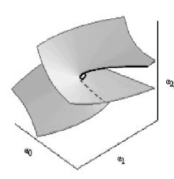
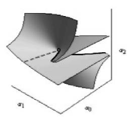
Figure 3: Two views of surface (46) in $\mathbb{R}^{3}$, black curve: $(\alpha^{3},3\alpha^{2},3\alpha)$, dashed curve: $(-\alpha^{3},-\alpha^{2},\alpha)$

It is remarkable that two curves on the surface (46) give rise to maps related to the Boussinesq and the matrix KdV equation.

4.1.1 A 4-parametric symplectic Y-B map

If we set the values (2) to $X$, in order to restrict on the level sets of the Casimir functions of $\mathcal{L}^{3}_{I}$ we set $f_{2}(X;I)=\alpha_{2},\ f_{1}(X;I)=\alpha_{1}$ (of course $f_{0}(X;I)$ will be also constant since (46) must be satisfied) and solve (4.1) with respect to $x_{22}$ and $x_{33}$ to get

$$x_{22}=\frac{\alpha_{2}}{3}+\frac{x_{12}x_{23}}{x_{13}}\pm\frac{1}{3}\sqrt{\alpha_{2}^{2}-3\alpha_{1}}\ ,\ x_{33}=\frac{\alpha_{2}}{3}-\frac{x_{13}x_{21}}{x_{23}}-\frac{x_{12}x_{23}}{x_{13}}\mp\frac{2}{3}\sqrt{\alpha_{2}^{2}-3\alpha_{1}}\ .$$

For simplicity we can change the parameters into $c_{1}=\frac{\alpha_{2}}{3}$ and $c_{2}=\pm\frac{1}{3}\sqrt{\alpha_{2}^{2}-3\alpha_{1}}$, so $x_{22}=c_{1}+c_{2}+\frac{x_{12}x_{23}}{x_{13}},\ x_{33}=c_{1}-2c_{2}-\frac{x_{13}x_{21}}{x_{23}}-\frac{x_{12}x_{23}}{x_{13}}$. Substituting these values to (2) and the new $x_{ij}$ to $X-\zeta I$, we obtain the two parametric family of matrices

$M(x_{12},x_{13},x_{21},x_{23};c_{1},c_{2})$

$$=\begin{pmatrix}\frac{x_{13}x_{21}}{x_{23}}+c_{1}+c_{2}-\zeta&x_{12}&x_{13}\\ x_{21}&\frac{x_{12}x_{23}}{x_{13}}+c_{1}+c_{2}-\zeta&x_{23}\\ -\frac{x_{13}x_{21}^{2}}{x_{23}^{2}}-\frac{3c_{2}x_{21}}{x_{23}}-\frac{x_{12}x_{21}}{x_{13}}&-\frac{x_{23}x_{12}^{2}}{x_{13}^{2}}-\frac{3c_{2}x_{12}}{x_{13}}-\frac{x_{21}x_{12}}{x_{23}}&c_{1}-2c_{2}-\frac{x_{13}x_{21}}{x_{23}}-\frac{x_{12}x_{23}}{x_{13}}-\zeta\end{pmatrix}$$ (48)

The reduced Poisson structure is

$$\{x_{12},x_{21}\}=\frac{x_{12}x_{23}}{x_{13}}-\frac{x_{13}x_{21}}{x_{23}},\ \{x_{12},x_{23}\}=-x_{13},\ \{x_{13},x_{21}\}=x_{23}$$

and $\{x_{12},x_{13}\}=\{x_{13},x_{23}\}=\{x_{21},x_{23}\}=0$, which defines the symplectic form :

$$\omega=\frac{1}{x_{23}}dx_{13}\wedge dx_{21}-\frac{1}{x_{13}}dx_{12}\wedge dx_{23}+(\frac{x_{12}}{x_{13}^{2}}-\frac{x_{21}}{x_{23}^{2}})dx_{13}\wedge dx_{23}\ .$$

We can change to canonical variables by setting

$$x_{13}=X_{1},\ x_{23}=X_{2},\ x_{21}=-x_{1}X_{2},\ x_{12}=-x_{2}X_{1}.$$ (49)

Then we denote matrix $M(x_{12},x_{13},x_{21},x_{23};c_{1},c_{2})$ by
$L(x_{1},x_{2},X_{1},X_{2};c_{1},c_{2})\equiv L^{\prime}_{I}(x_{1},x_{2},X_{1},X_{2};\alpha_{1},\alpha_{2})-\zeta I$

$$\equiv\begin{pmatrix}c_{1}+c_{2}-x_{1}X_{1}-\zeta&-X_{1}x_{2}&X_{1}\\ -x_{1}X_{2}&c_{1}+c_{2}-x_{2}X_{2}-\zeta&X_{2}\\ -x_{1}(x_{1}X_{1}+x_{2}X_{2}-3c_{2})&-x_{2}(x_{1}X_{1}+x_{2}X_{2}-3c_{2})&c_{1}-2c_{2}+x_{1}X_{1}+x_{2}X_{2}-\zeta\end{pmatrix}$$ (50)

and the symplectic form $\omega$ by the canonical symplectic form $\omega_{0}=dx_{1}\wedge dX_{1}+dx_{2}\wedge dX_{2}.$

From the re-factorization formula (28), (29), for $K_{\alpha}=K_{\beta}=I$, $X=L^{\prime}_{I}(x_{1},x_{2},X_{1},X_{2};\alpha_{1},\alpha_{2})$ and $Y=L^{\prime}_{I}(y_{1},y_{2},Y_{1},Y_{2};\beta_{1},\beta_{2})$, since the Casimir functions on

$$\Sigma_{I}(\alpha_{1},\alpha_{2})=\{L(x_{1},x_{2},X_{1},X_{2};\alpha_{1},\alpha_{2})\ |\ x_{1},x_{2},X_{1},X_{2}\in\mathbb{C}\}$$

are

$$f_{0}(X;I)=(\alpha_{1}-2\alpha_{2})(a_{1}+a_{2})^{2},\ f_{1}(X;I)=3(\alpha_{1}^{2}-\alpha_{2}^{2}),\ f_{2}(X;I)=3\alpha_{1},$$

we obtain the matrices

$$U=(YX(3\alpha_{1}I-Y-X)-(\alpha_{1}-2\alpha_{2})(a_{1}+a_{2})^{2}I)((3\alpha_{1}I-Y-X)(Y+X)+YX-3(\alpha_{1}^{2}-\alpha_{2}^{2})I)^{-1},$$

$V=Y+X-U$.
If we denote by $U_{ij},V_{ij}$ the elements of the matrices $U$ and $V$, we come up to the next proposition.

Proposition 4.4.

The map

$R_{((\alpha_{1},\alpha_{2}),(\beta_{1},\beta_{2}))}:((x_{1},x_{2},X_{1},X_{2}),(y_{1},y_{2},Y_{1},Y_{2}))\mapsto((u_{1},u_{2},U_{1},U_{2}),(v_{1},v_{2},V_{1},V_{2}))$ where

$$U_{1} = U_{13},\ U_{2}=U_{23},\ u_{1}=-\frac{U_{21}}{U_{23}},\ u_{2}=-\frac{U_{12}}{U_{13}},$$

$$V_{1} = V_{13},\ V_{2}=V_{23},\ \ v_{1}=-\frac{V_{21}}{V_{23}},\ v_{2}=-\frac{V_{12}}{V_{13}}$$

is a symplectic parametric Yang-Baxter map, with respect to the canonical symplectic form $dx_{1}\wedge dX_{1}+dx_{2}\wedge dX_{2}+dy_{1}\wedge dY_{1}+dy_{2}\wedge dY_{2}$, and admits the strong Lax matrix $L(x_{1},x_{2},X_{1},X_{2};\alpha_{1},\alpha_{2})$.

Proof:

The YB property of this map can be checked by direct computation. Moreover $u_{i},\ U_{i},\ v_{i},\ V_{i},\ i=1,2$ is the unique solution (proposition 4.1) of the Lax equation:

$$L(u_{1},u_{2},U_{1},U_{2};\alpha_{1},\alpha_{2})L(v_{1},v_{2},V_{1},V_{2};\beta_{1},\beta_{2})=L(y_{1},y_{2},Y_{1},Y_{2};\beta_{1},\beta_{2})L(x_{1},x_{2},X_{1},X_{2};\alpha_{1},\alpha_{2})$$

The explicit formula of the YB map $R_{((\alpha_{1},\alpha_{2}),(\beta_{1},\beta_{2}))}$ of proposition 4.4 is

$$(u_{1},u_{2}) = (y_{1},y_{2})-\frac{\alpha_{1}-\beta_{1}-2(\alpha_{2}-\beta_{2})}{D}\ (x_{1}-y_{1},x_{2}-y_{2}),$$

$$(v_{1},v_{2}) = (x_{1},x_{2})+\frac{\alpha_{1}-\beta_{1}+\alpha_{2}-\beta_{2}}{D}\ \ (x_{1}-y_{1},x_{2}-y_{2}),$$

with $D=2\alpha_{2}-\alpha_{1}+\beta_{1}+\beta_{2}+y_{1}X_{1}+y_{2}X_{2}-x_{1}X_{1}-x_{2}X_{2}$, and

$$U_{1}=\frac{(x_{1}-v_{1})X_{1}+(y_{1}-v_{1})Y_{1}}{u_{1}-v_{1}},\ \ U_{2}=\frac{(x_{2}-v_{2})X_{2}+(y_{2}-v_{2})Y_{2}}{u_{2}-v_{2}},$$

$$V_{1}=\frac{(x_{1}-u_{1})X_{1}+(y_{1}-u_{1})Y_{1}}{v_{1}-u_{1}},\ \ V_{2}=\frac{(x_{2}-u_{2})X_{2}+(y_{2}-u_{2})Y_{2}}{v_{2}-u_{2}}.$$

We will point out two special cases of this YB map that give rise to Boussinesq and Goncharenko–Veselov maps.

4.1.2 The Boussinesq Y-B map ($\alpha_{0}=\alpha^{3},\ \alpha_{1}=3\alpha^{2},\ \alpha_{2}=3\alpha$)

By setting $c_{2}=0,\ c_{1}=\alpha$ to (50) we derive the Lax matrix

$$L_{B}(x_{1},x_{2},X_{1},X_{2};\alpha)=\begin{pmatrix}\alpha-\zeta-x_{1}X_{1}&-X_{1}x_{2}&X_{1}\\ -x_{1}X_{2}&\alpha-\zeta-x_{2}X_{2}&X_{2}\\ -x_{1}(x_{1}X_{1}+x_{2}X_{2})&-x_{2}(x_{1}X_{1}+x_{2}X_{2})&\alpha-\zeta+x_{1}X_{1}+x_{2}X_{2}\end{pmatrix}$$

In this case the Casimir functions on $\Sigma_{I}(\alpha)=\{L^{B}(x_{1},x_{2},X_{1},X_{2};\alpha)\ /\ x_{1},x_{2},X_{1},X_{2}\in\mathbb{C}\}$ are

$$f_{0}(X;I)=\alpha^{3},\ f_{1}(X;I)=3\alpha^{2},\ f_{2}(X;I)=3\alpha,$$

for $X=L_{I}^{B}(x_{1},x_{2},X_{1},X_{2};\alpha)\equiv L_{B}(x_{1},x_{2},X_{1},X_{2};\alpha)+\zeta I$. The curve $(\alpha^{3},3\alpha^{2},3\alpha)$ is depicted in fig. 3 with black color.

The corresponding 2-parametric YB map $R^{B}_{\alpha,\beta}$ with strong Lax matrix $L_{B}(x_{1},x_{2},X_{1},X_{2};c)$ is induced from the YB map $R_{((\alpha_{1},\alpha_{2}),(\beta_{1},\beta_{2}))}$ of proposition 4.1 i.e. $R^{B}_{\alpha,\beta}=R_{((\alpha,0),(\beta,0))}$ .

4.1.3 The Goncharenko–Veselov map ($\alpha_{0}=-\alpha^{3},\ \alpha_{1}=-\alpha^{2},\alpha_{2}=\alpha$)

In a similar way if we set $c_{1}=\frac{\alpha}{3}$ and $c_{2}=\frac{2\alpha}{3}$ we obtain the Yang-Baxter map

$$R^{GV}_{\alpha,\beta}=R_{((\frac{\alpha}{3},\frac{2\alpha}{3}),(\frac{\beta}{3},\frac{2\beta}{3}))}$$

with strong Lax matrix

$$L_{GV}(\mathbf{x};\alpha)=\begin{pmatrix}\alpha-\zeta-x_{1}X_{1}&-X_{1}x_{2}&X_{1}\\ -x_{1}X_{2}&\alpha-\zeta-x_{2}X_{2}&X_{2}\\ -x_{1}(x_{1}X_{1}+x_{2}X_{2}-2\alpha)&-x_{2}(x_{1}X_{1}+x_{2}X_{2}-2\alpha)&x_{1}X_{1}+x_{2}X_{2}-\alpha-\zeta\end{pmatrix}$$

for $\mathbf{x}=(x_{1},x_{2},X_{1},X_{2})$. Here for $X=L_{GV}(\mathbf{x};\alpha)+\zeta I$, $(f_{0}(X;I),f_{1}(X;I),f_{2}(X;I))=(-\alpha^{3},-\alpha^{2},\alpha)$, which is the dashed curve of fig. 3.

Both maps $R^{B}_{\alpha,\beta}$ and $R^{GV}_{\alpha,\beta}$ are symplectic with respect to the canonical symplectic form $dx_{1}\wedge dX_{1}+dx_{2}\wedge dX_{2}+dy_{1}\wedge dY_{1}+dy_{2}\wedge dY_{2}$.

In [8], Goncharenko and Veselov presented a YB map as interaction of two soliton solutions of the matrix KdV equation and claimed that it admits the Lax matrix of the form:

$$A(\xi,\eta;\lambda)=I+\frac{2\lambda}{\zeta-\lambda}\frac{\xi\otimes\eta}{(\xi,\eta)}\ ,$$ (51)

for the n-dimensional vectors $\xi$ and $\eta$. Here $\lambda$ is the YB parameter. Essentially $\xi,\eta\in\mathbb{C}P^{n-1}$ since $\xi\mapsto\mu\xi$, $\eta\mapsto\nu\eta$ leaves (51) invariant. Even if the case for $n=2$ is rather trivial, it is quite interesting for higher dimensions.

First we observe that we can multiply the Lax matrix (51) with ${\zeta-\lambda}$ and change $\zeta$ with $-\zeta$ in order to derive an equivalent Lax matrix

$$B(\xi,\eta;\lambda)=\lambda(2\ \frac{\xi\otimes\eta}{(\xi,\eta)}-I)-\zeta I$$

for the same YB map. Now, let $n=3$, $\xi=(\xi_{1},\xi_{2},\xi_{3})$ and $\eta=(\eta_{1},\eta_{2},\eta_{3})$. Considering the affine part of $\mathbb{C}P^{2}$, we have $\xi=(\xi_{1},\xi_{2},1)$, $\eta=(\eta_{1},\eta_{2},1)$ and by performing the invertible transformation $(\eta_{1},\eta_{2},\xi_{1},\xi_{2},)\mapsto(x_{1},x_{2},X_{1},X_{2})$:

$$x_{1}=-\eta_{1}\ ,\ x_{2}=-\eta_{2}\ ,\ X_{1}=\frac{2\alpha\xi_{1}}{\xi_{1}\eta_{1}+\xi_{2}\eta_{2}+1}\ ,\ X_{2}=\frac{2\alpha\xi_{2}}{\xi_{1}\eta_{1}+\xi_{2}\eta_{2}+1}\ ,$$

the matrix $B(\xi,\eta;\lambda)$ is transformed to the Lax matrix $L_{GV}(\mathbf{x};-\lambda)$.

5 Conclusion

By generalizing the re-factorization procedure reported in [9], we presented a construction of multidimensional parametric Yang-Baxter maps. The symplectic quadrirational YB maps on $\mathbb{C}^{2}\times\mathbb{C}^{2}$, that was derived in this way, where classified in two cases (three cases for real maps). The re-factorization of $3\times 3$ binomial matrices provided us a family of symplectic YB maps on $\mathbb{C}^{4}\times\mathbb{C}^{4}$ with Lax matrices the four dimensional symplectic leaves of $\mathcal{L}^{3}_{I}$.

A similar classification procedure with the one presented here for quadrirational YB maps with $n\times n$ binomial Lax matrices, for $n>2$, is a far more difficult task. The determination of the commuting pairs of invertible $n\times n$ matrices, in addition with the determination of the corresponding symplectic leaves on $\mathcal{L}^{n}$, is needed. It would be interesting to investigate this problem for small values of $n$. Furthermore other re-factorization formulas of higher degree polynomial matrices, guided by the invariance of the Casimir functions of the Sklyanin bracket, could lead to symplectic multidimensional YB maps. The derived maps contain, in general, more than one YB parameters. One can ask if (some of) these parameters are associated to spectral ones, in view of the 3D consistency of the YB maps. This is an interesting question especially with respect to finding invariants of the corresponding transfer maps and is going to be investigated in the future. Other issues deserving further research are initial value problems on lattices connected to the maps reported here, as well as the study of their continuum limits.

acknowledgments

TEK acknowledges partial support from the State Scholarships Foundation of Greece. Both authors thank the anonymous referee for useful comments.

References

- [1] V.E. Adler, A.I. Bobenko, Yu.B. Suris, Classification of integrable equations on quad-graphs. The consistency approach, Comm. Math. Phys. 233, 2003, 513–543.
- [2] V.E. Adler, A.I. Bobenko, Yu.B. Suris, Geometry of Yang-Baxter maps: pencils of conics and quadrirational mappings, Comm. Anal. Geom. 12, 2004, 967–1007.
- [3] V.E. Adler, R.I. Yamilov, Explicit auto-transformations of integrable chains, J. Phys. A: Math. Gen. 27, 1994, 477–492.
- [4] A.I. Bobenko, Yu.B. Suris, Integrable systems on quad-graphs, Int. Math. Res. Notices, No. 11, 2002, 573–611.
- [5] V.G. Drinfeld, On some Unsolved Problems in Quantum Group Theory, Lecture Notes in Math. 1510, 1992, 1–8.
- [6] P. Etingof, T. Schedler, A. Soloviev, Set-theoretical solutions to the quantum Yang-Baxter equation, Duke Math. J. 100 no. 2, 1999, 169–209.
- [7] P. Etingof, Geometric crystals and set-theoretical solutions to the quantum Yang-Baxter equation, Comm. Algebra, 31 no. 4, 2003, 1961–1973
- [8] V.M. Goncharenko, A.P. Veselov, Yang-Baxter maps and matrix solitons, NATO Sci. Ser. II Math. Phys. Chem., 132. New trends in integrability and partial solvability, 2004, 191–197.
- [9] T.E. Kouloukas, V.G. Papageorgiou, Yang-Baxter maps with first-degree-polynomial Lax matrices, J. Phys. A: Math. Theor. 42, 2009, 404012
- [10] T.E. Kouloukas, V.G. Papageorgiou, Entwining Yang-Baxter maps and integrable lattices, arXiv:1006.2145v1.
- [11] J.-H. Lu , M. Yan, Y.-C.Zhu, On the set–theoretical Yang–Baxter equation, Duke Math. J. 104, 2000, 1–18.
- [12] F.W. Nijhoff, Lax pair for the Adler (lattice Krichever-Novikov) system, Phys. Lett. A, 297, 2002, 49–58.
- [13] V.G. Papageorgiou, F.W. Nijhoff, H.W. Capel, Integrable mappings and nonlinear integrable lattice equations, Phys. Lett. A, 147, 1990, 106–114.
- [14] V.G. Papageorgiou, Yu.B. Suris, A.G. Tongas, A.P. Veselov, On Quadrirational Yang-Baxter Maps, SIGMA 6, 033, 2010, 9p.
- [15] V.G. Papageorgiou, A.G. Tongas, A.P. Veselov, Yang-Baxter maps and symmetries of integrable equations on quad-graphs, J. Math. Phys. 47, 2006, 083502 1–16.
- [16] V.G. Papageorgiou, A.G. Tongas, Yang-Baxter maps and multi-field integrable lattice equations, J. Phys. A 40, no. 42, 2007, 12677–12690.
- [17] N. Reshetikhin, A.P. Veselov, Poisson Lie groups and Hamiltonian theory of the Yang–Baxter maps, math.QA/0512328, 2005.
- [18] M. Semenov-Tian-Shansky, Dressing transformations and Poisson group actions, Publ. RIMS, Kyoto University, 21, 1985, 1237–1260.
- [19] E.K Sklyanin, Some algebraic structures connected with the Yang-Baxter equation, Funct. Anal. Appl. 16, No 4, 1983, 263–270.
- [20] E.K Sklyanin, Classical limits of SU(2)–invariant solutions of the Yang-Baxter equation, J. Soviet Math. 40, No 1, 1988, 93–107.
- [21] Yu.B. Suris, A.P. Veselov, Lax matrices for Yang–Baxter maps, J. Nonlin. Math. Phys. 10, suppl.2, 2003, 223–230.
- [22] A.P. Veselov, Yang-Baxter maps and integrable dynamics, Phys. Lett. A, 314, 2003, 214–221.
- [23] A.P. Veselov, Yang-Baxter maps: dynamical point of view, Combinatorial Aspects of Integrable Systems (Kyoto, 2004), MSJ Mem. vol 17, 2007, pp 145–67.
- [24] A. Weinstein, P. Xu, 1992 Classical solutions to the Quantum Yang–Baxter equation, Commun. Math. Phys. 148, 1992, 309–343.