Bias-Controlled Selective Excitation of Vibrational Modes in Molecular Junctions: A Route Towards Mode-Selective Chemistry

Abstract

We show that individual vibrational modes in single-molecule junctions with asymmetric molecule-lead coupling can be selectively excited by applying an external bias voltage. Thereby, a non-statistical distribution of vibrational energy can be generated, that is, a mode with a high frequency can be stronger excited than a mode with a lower frequency. This is of particular interest in the context of mode-selective chemistry, where one aims to break specific (not necessarily the weakest) chemical bond in a molecule. Such Mode-Selective Vibrational Excitation is demonstrated for two generic model systems representing asymmetric molecular junctions and/or Scanning Tunneling Microscopy experiments. To this end, we employ two complementary theoretical approaches, a nonequilibrium Green’s function approach and a master equation approach. The comparison of both methods reveals good agreement in describing resonant electron transport through a single-molecule contact, but also highlights the role of non-resonant transport processes, in particular co-tunneling and off-resonant electron-hole pair creation processes.

I Introduction

Mode-selective chemistry, that is the control of specific conformational changes or chemical reactions by directing energy into specific vibrational modes of a molecule, has been a major goal and challenge of modern chemical physics Jortner et al. (1991); Liu et al. (2006); Crim (2008). A variety of different routes to achieve mode-selective chemistry have been considered. For example, ultrafast excitation of molecules by laser pulses provided a route for directing energy transiently into specific mode-excitation or bond-cleavage in the presence of Intramolecular Vibrational Energy Redistribution (IVR) processes Potter et al. (1992); Zare (1998); Brumer and Shapiro (2003). Nevertheless, on long time scales the statistical distribution of energy usually prevails and the control of specific conformational changes or chemical reactions by directing energy into specific vibrational modes still represents a challenge Bryan et al. (2011).

In recent years, much interest has been devoted to the study of molecular systems out of equilibrium, in particular single-molecule junctions Joachim and Roth (1997); Park et al. (2000); Reichert et al. (2002); Smit et al. (2002); Nitzan and Ratner (2003); Pascual et al. (2003); Wu et al. (2004); Ogawa et al. (2007); Hihath et al. (2008); Schulze et al. (2008); Pump et al. (2008); Ballmann et al. (2010); Osorio et al. (2010); Hihath et al. (2010); Cuevas and Scheer (2010); Secker et al. (2011). These junctions consist of a single molecule that is clamped between two metal or semi-conductor electrodes. If these electrodes are set to different electrochemical potentials by applying an external bias voltage, electrons tunnel from one lead to the other trough the molecule. The geometrical structure of the molecular bridge, due to its small size and mass, is very sensitive to charge fluctuations induced by these tunneling processes. The tunneling electrons thus strongly interact with the vibrational degrees of freedom of the junction Wu et al. (2004); Yu et al. (2004); Huang et al. (2006); Ward et al. (2008); Repp et al. (2010); Ballmann et al. (2010); Hihath et al. (2010); Osorio et al. (2010); Secker et al. (2011). The distribution of vibrational energy on the molecular bridge, which results from these interactions, is highly correlated with the applied bias voltage and often deviates from a Boltzmann distribution Mitra et al. (2004); Koch et al. (2006); Koch and von Oppen (2005); Ward et al. (2008); Ioffe et al. (2008); Härtle et al. (2008, 2009, 2010); Härtle and Thoss (2011a); Entin-Wohlman et al. (2010); Härtle and Thoss (2011b); Härtle et al. (2011). In a single-molecule junction, it is thus possible to control a ”non-statistical” non-equilibrium distribution of vibrational energy by an external potential bias. This offers an alternative route to mode-selective excitation (or mode-selective chemistry). Moreover, in the steady-state transport regime of a molecular junction, this could be achieved even without the cumbersome preparation of a specific initial-state.

Employing generic model systems, we have recently shown Härtle et al. (2010) that in a single-molecule junction the excitation of vibrational modes can be, indeed, selectively controlled by the external bias voltage. Considering molecules with an asymmetric orbital structure and vibronic coupling to specific normal modes, it was demonstrated that, by adjusting the external bias voltage, such a system can be driven into different non-equilibrium states with different levels of excitation for specific nuclear modes. Particularly, the excitation of a high frequency mode can be tuned much higher than that of a low frequency mode, thus overcoming the statistical distribution of vibrational energy that favors the excitation of low frequency modes. In this article, we extend our previous studies Härtle et al. (2010), where the principle of Mode-Selective Vibrational Excitation (MSVE) in a single-molecule junction was demonstrated for the first time. To this end, we outline in detail how the excitation of a single vibrational mode can be controlled by an external bias voltage. This bias-controlled excitation is then generalized to more than one vibrational mode, reviewing the basic MSVE phenomenon and emphasizing the role of intra-molecular interactions. In particular, we demonstrate MSVE in the presence of electronically mediated mode-mode coupling Härtle et al. (2008), which results from coupling of the vibrational modes to the same electronic state. These interactions induce energy transfer between the vibrational modes and tend to distribute current-induced vibrational excitation between the different modes. Similarly, electronic correlations, e.g. due to Coulomb repulsion, may influence MSVE by reorganizing the electronic population between specific electronic states at the molecule, which, to some extent and in different ways, is related to the phenomenon of MSVE. Extending our previous work, we investigate complementary models for asymmetric molecular junctions exhibiting MSVE. These models are related, for example, to experiments on single-molecule junctions performed with a Scanning Tunneling Microscope (STM) Gaudioso et al. (2000); Pascual et al. (2003); Choi et al. (2006); Ogawa et al. (2007); Pump et al. (2008); Lafferentz et al. (2009); Schulze et al. (2008); Repp et al. (2010).

To describe this nonequilibrium transport problem, we employ two complementary approaches. The first one is a Master Equation approach (ME) that is based on the time-evolution of the reduced density matrix of the molecular bridge May (2002); Mitra et al. (2004); Lehmann et al. (2004); Ovchinnikov and Neuhauser (2005); Pedersen and Wacker (2005); Welack et al. (2006); Harbola et al. (2006); Zazunov et al. (2006); Siddiqui et al. (2007); Timm (2008); May and Kühn (2008a, b); Leijnse and Wegewijs (2008); Esposito and Galperin (2009, ); Peskin (2010); Härtle et al. (2010); Härtle and Thoss (2011a); Pshenichnyuk and Cizek (2011); Volkovich and Peskin (2011); Härtle and Thoss (2011b). The respective equation of motion is evaluated strictly to second-order in the molecule-lead coupling, for which all resonant transport processes are included. Within such a framework, no approximations with respect to the interactions on the molecular bridge need to be invoked, in particular not with respect to electron-electron interactions or electronic-vibrational coupling. However, higher-order processes König et al. (1996); Paaske and Flensberg (2005); Sela et al. (2006); Galperin et al. (2007); Lüffe et al. (2008); Härtle et al. (2008); Leijnse et al. (2009); Han (2010) like co-tunneling processes or the broadening of molecular levels due to the molecule-lead coupling are missing in this description. Note that master equation approaches that take into account such higher-order effects have already been put forward May (2002); Pedersen and Wacker (2005); Leijnse and Wegewijs (2008); Esposito and Galperin (2009, ). In the present work, however, we selected a Nonequilibrium Green’s Function approach (NEGF) Flensberg (2003); Mitra et al. (2004); Galperin et al. (2006); Ryndyk et al. (2006); Frederiksen et al. (2007); Tahir and MacKinnon (2008); Härtle et al. (2008); Avriller and Levy Yeyati (2009); Schmidt and Komnik (2009); Haupt et al. (2009); Bergfield and Stafford (2009); Härtle et al. (2009); Kubala and Marquardt (2010); Härtle et al. (2010, 2011) to account for the higher-order effects. Especially for the description of multiple vibrational modes Härtle et al. (2008, 2010); Secker et al. (2011), the NEGF methodology is typically more efficient. We employ a nonequilibrium Green’s function approach, which was originally proposed by Galperin et al. Galperin et al. (2006) and recently extended to account for multiple vibrational and multiple electronic degrees of freedom of the molecular bridge Härtle et al. (2008, 2009, 2010, 2011). Other theoretical approaches used to describe electron transport through a single-molecule junction are based e.g. on scattering theory Cizek et al. (2004, 2005); C-C. Kaun and Seideman (2005); Caspary Toroker and Peskin (2007); Benesch et al. (2008); Zimbovskaya and Kuklja (2009); Jorn and Seidemann (2009), path integrals Mühlbacher and Rabani (2008); Weiss et al. (2008); Segal et al. (2010), multiconfigurational wave-function methods Wang and Thoss (2009); Velizhanin et al. (2010); Wang and Thoss (2011), flux-correlation approaches Caspary Toroker and Peskin (2010) or exact diagonalization Hackl et al. (2009).

The paper is organized as follows. The Hamiltonian that we use to describe electron transport through a single-molecule junction is outlined in Sec. II.1. The ME and NEGF methodologies that we employ to calculate steady-state observables of a biased single-molecule junction are briefly described in Secs. II.2 and II.3, respectively. The basic physical mechanisms for vibrational heating and cooling in an asymmetric molecular junction, which lead to MSVE, are reviewed and analyzed for a single-level conductor in Sec. III.1. Thereby, the role of electron-hole pair creation processes, which constitutes an important cooling mechanism in a molecular junction Härtle et al. (2010); Härtle and Thoss (2011a, b), is discussed in detail. Moreover, the comparison of results obtained from our NEGF and ME schemes enables us to distinguish resonant and non-resonant contributions. In Sec. III.2, we discuss MSVE in two model systems, representing generic asymmetric molecular junctions: A single-molecule junction with an intrinsically asymmetric molecular bridge (model A) Härtle et al. (2010), and a junction, where the bridging molecule is asymmetrically coupled to the leads (model B). The latter scenario is typical for STM experiments. We demonstrate that the magnitude and the polarity of the external bias voltage can be used to direct vibrational energy into specific vibrational modes, even in the presence of intra-molecular interactions that tend to suppress the effect. Thus, we predict that in the steady-state transport regime of a molecular junction, a bias-controlled ”non-statistical” distribution of vibrational energy can be realized, where modes with higher frequency (stronger bonds) can be much higher excited than modes with a lower frequency (weaker bonds).

II Theoretical Methodology

II.1 Model Hamiltonian

We consider electron transport through a single molecule that is covalently bound to two metal leads. To this end, we employ a generic model Hamiltonian

$$\hat{H} = \hat{H}_{\text{el}}+\hat{H}_{\text{vib}},$$ (1)

describing the electronic, $\hat{H}_{\text{el}}$, and the vibrational degrees of freedom, $\hat{H}_{\text{vib}}$, of this transport problem.

The electronic part of $\hat{H}$ can be represented by a discrete set of electronic states, located at the molecular bridge (M), and by a continuum of electronic states describing the electron reservoirs of the left (L) and the right (R) electrode. Tunneling of electrons from one lead to the other is described by the following model Hamiltonian ($\hbar=1$):

$$\hat{H}_{\text{el}} = \sum_{m\in\text{M}}{\epsilon_{m}a_{m}^{\dagger}a_{m}}+\sum_{m<n\in\text{M}}{U_{m,n}a_{m}^{\dagger}a_{m}a_{n}^{\dagger}a_{n}}$$

$$+\sum_{k\in\text{L,R}}{\epsilon_{k}b_{k}^{\dagger}b_{k}}+\sum_{K\in\text{L,R};k\in K;m\in\text{M}}{(\upsilon_{K,m}\xi_{K,k}b_{k}^{\dagger}a_{m}+h.c.)}.$$

The energies of the electronic states in the leads, which are addressed by creation and annihilation operators $b_{k}^{\dagger}$ and $b_{k}$, are denoted by $\epsilon_{k}$. The energy of the $m$th electronic state located at the molecular bridge is given by $\epsilon_{m}$. These states are populated with creation operators $a_{m}^{\dagger}$ and depopulated with annihilation operators $a_{m}$. The molecular bridge is bilinearly coupled to the electrodes, $\sim b_{k}^{\dagger}a_{m}$, with coupling strengths $\upsilon_{K,m}\xi_{K,k}$. For simplicity, these coupling strengths are factorized into an electrode term, $\xi_{K,k}$, which determines the electrode’s ($K$=L,R) spectral density, $J_{K}(\epsilon)=\sum_{k\in K}|\xi_{K,k}|^{2}\delta(\epsilon-\epsilon_{k})$, and a molecular term, which represents the coupling of the $m$th molecular state to the $K$th electrode, $\upsilon_{K,n}$. To model the leads we use a semi-elliptic conduction-band with a band-width of $4\gamma$ such that the corresponding level-width functions read:

$$\Gamma_{K,mn}(\epsilon)=2\pi\upsilon_{K,m}\upsilon_{K,n}J_{K}(\epsilon)=\upsilon_{K,m}\upsilon_{K,n}\frac{\xi^{2}}{{\gamma}^{2}}\sqrt{4\gamma^{2}-{(\epsilon-\mu_{K})}^{2}}.$$ (3)

Charging energies, e.g. due to Coulomb interactions, are accounted for by Hubbard-like electron-electron interaction terms, $U_{m,n}a_{m}^{\dagger}a_{m}a_{n}^{\dagger}a_{n}$. The Fermi-energy of the overall system is given by $\epsilon_{\text{F}}=0$  eV.

Vibrational degrees of freedom of the molecule are described as harmonic oscillators,

$$\hat{H}_{\text{vib}} = \sum_{\nu}\Omega_{\nu}c_{\nu}^{\dagger}c_{\nu}+\sum_{m\in\text{M};\nu}\lambda_{\nu,m}q_{\nu}a_{m}^{\dagger}a_{m}$$ (4)

$$+\sum_{\nu,\beta_{\nu}}\omega_{\beta_{\nu}}d_{\beta_{\nu}}^{\dagger}d_{\beta_{\nu}}+\sum_{\nu,\beta_{\nu}}\eta_{\nu,\beta_{\nu}}(d_{\beta_{\nu}}^{\dagger}+d_{\beta_{\nu}})(c_{\nu}^{\dagger}+c_{\nu}),$$

where the ladder operators $c^{\dagger}_{\nu}$/$c_{\nu}$ address the $\nu$th vibrational (normal) mode of the molecular bridge with frequency $\Omega_{\nu}$. Changes in the nuclear potential energy surface due to electronic transitions between the single particle states are assumed to be linear in both the vibrational displacements, $q_{\nu}=\frac{1}{\sqrt{2}}(c_{\nu}+c_{\nu}^{\dagger})$, and the electronic densities, $a_{m}^{\dagger}a_{m}$. The respective coupling strengths are given by $\lambda_{\nu,m}$. To incorporate vibrational relaxation effects in a phenomenological way Weiss (1993); Thoss and Domcke (1998), each intramolecular vibrational mode is coupled to a thermal bath. The creation and annihilation operator for a bath mode with frequency $\omega_{\beta_{\nu}}$ are denoted by $d^{\dagger}_{\beta_{\nu}}$ and $d_{\beta_{\nu}}$, respectively. The corresponding mode-bath coupling strengths are given by $\eta_{\nu,\beta_{\nu}}$. All properties of the bath that influence the dynamics of the system are determined by the spectral densities $J_{\nu}(\omega)=\sum_{\beta_{\nu}}\eta_{\nu,\beta_{\nu}}^{2}\delta(\omega-\omega_{\beta_{\nu}})$. In the calculations presented below, we use an Ohmic bath model with a cutoff frequency, $\omega_{c,{\nu}}$, and

$$J_{\nu}(\omega)=\frac{\zeta_{\nu}^{2}}{\omega_{c,\nu}^{2}}\omega e^{-\omega/\omega_{c,\nu}}.$$ (5)

II.2 Reduced Density Matrix Approach

Weak coupling of the molecule to the electron reservoirs (the leads), as well as to the energy reservoirs (the nuclear bath modes), is essential in order to relate the junction’s steady-state observables to intrinsic properties of the molecular bridge Caspary Toroker and Peskin (2009). For this purpose it is instructive to regroup the different terms in the Hamiltonian into the molecular ”system”, which include the molecular electronic states and vibrational modes, and ”bath” terms, which include the electron reservoirs and the nuclear baths. The full Hamiltonian is therefore rewritten as:

$$\hat{H} = \hat{H}_{\text{S}}+\hat{H}_{\text{B}}+\hat{H}_{\text{SB}},$$ (6)

with

$$\hat{H}_{\text{S}}= \sum_{m\in\text{M}}{\epsilon_{m}a_{m}^{\dagger}a_{m}}+\sum_{m<n\in\text{M}}{U_{m,n}a_{m}^{\dagger}a_{m}a_{n}^{\dagger}a_{n}}+\sum_{\nu}{\Omega_{\nu}c_{\nu}^{\dagger}c_{\nu}}+\sum_{m\in\text{M};\nu}{\lambda_{\nu,m}q_{\nu}a_{m}^{\dagger}a_{m}},$$ (7)

$$\hat{H}_{\text{B}}= \sum_{k\in\text{L,R}}{\epsilon_{k}b_{k}^{\dagger}b_{k}}+\sum_{\nu,\beta_{\nu}}{\omega_{\beta_{\nu}}d_{\beta_{\nu}}^{\dagger}d_{\beta_{\nu}}},$$ (8)

$$\hat{H}_{\text{SB}}= \sum_{\nu,\beta_{\nu}}{\eta_{\nu,\beta_{\nu}}(d_{\beta_{\nu}}^{\dagger}+d_{\beta_{\nu}})(c_{\nu}^{\dagger}+c_{\nu})}+\sum_{K\in\text{L,R};k\in K;m\in\text{M}}{(\upsilon_{K,m}\xi_{K,k}.b_{k}^{\dagger}a_{m}+h.c.)}$$ (9)

The steady-state of the system under bias can be calculated by following the time-evolution of the system to its stationary state, starting from an arbitrary initial state. We consider an initial density matrix in a product form,

$$\hat{\rho}(0) = \hat{\rho}_{\text{S}}(0)\otimes\hat{\rho}_{\text{B}}(0),$$ (10)

$$\hat{\rho}_{\text{B}}(0) = \prod_{K\in\text{L,R}}{\hat{\rho}_{\text{B},K}}\otimes\prod_{\nu}{\hat{\rho}_{\text{B},\nu}},$$ (11)

where $\hat{\rho}_{\text{S}}(0)$ is any normalized system density matrix with $\text{tr}_{\text{S}}[\hat{\rho}_{\text{S}}(0)]=1$, and $\text{tr}_{\text{S}}[...]$ denotes the trace over the subspace of the molecular conductor. The electronic reservoirs are described by a product of equilibrium density operators,

$$\hat{\rho}_{\text{B},K}=\frac{e^{-\frac{1}{k_{\text{B}}T}\sum_{k\in K}{(\epsilon_{k}-\mu_{K})b^{\dagger}_{k}b_{k}}}}{\text{tr}[e^{-\frac{1}{k_{\text{B}}T}\sum_{k\in K}{(\epsilon_{k}-\mu_{K})b^{\dagger}_{k}b_{k}}}]},$$ (12)

with $K\in{\text{L,R}}$. Thus, we assume the leads to be in a thermal equilibrium state, which is characterized by the temperature $k_{\text{B}}T$ and the electrochemical potentials $\mu_{K}$. Similarly, the nuclear baths are represented by a product of equilibrium density operators,

$$\hat{\rho}_{\text{B},\nu}=\frac{e^{-\frac{1}{k_{\text{B}}T}\sum_{\beta_{\nu}}{\omega_{\beta_{\nu}}d^{\dagger}_{\beta_{\nu}}d_{\beta_{\nu}}}}}{\text{tr}[e^{-\frac{1}{k_{\text{B}}T}\sum_{\beta_{\nu}}{\omega_{\beta_{\nu}}d^{\dagger}_{\beta_{\nu}}d_{\beta_{\nu}}}}]},$$ (13)

where $\nu$ denotes the molecular mode to which the particular bath is coupled. The exact time-evolution of the full density operator is given by the Liouville-von Neumann equation,

$$\frac{\partial}{\partial t}\hat{\rho}(t)=-i[\hat{H},\hat{\rho}(t)].$$ (14)

Transforming the respective operators to the interaction representation,

$$\hat{O}^{\text{I}}(t)=e^{i[\hat{H}_{\text{S}}+\hat{H}_{\text{B}}]t}\hat{O}(t)e^{-i[\hat{H}_{\text{S}}+\hat{H}_{\text{B}}]t},$$ (15)

the Liouville-von Neumann equation can be rearranged to give Peskin (2010)

$$\frac{\partial}{\partial t}\hat{\rho}^{\text{I}}(t)=-i[\hat{H}^{\text{I}}_{\text{SB}}(t),\hat{\rho}^{\text{I}}(t)]-\int_{0}^{t}{\text{d}t^{\prime}[\hat{H}^{\text{I}}_{\text{SB}}(t),[\hat{H}^{\text{I}}_{\text{SB}}(t^{\prime}),\hat{\rho}^{\text{I}}(t)]]}$$

$$-i\int_{0}^{t}{\text{d}t^{\prime}\int_{t^{\prime}}^{t}{\text{d}t^{\prime\prime}[\hat{H}^{\text{I}}_{\text{SB}}(t),[\hat{H}^{\text{I}}_{\text{SB}}(t^{\prime}),[\hat{H}^{\text{I}}_{\text{SB}}(t^{\prime\prime}),\hat{\rho}^{\text{I}}(t^{\prime\prime})]]]}}.$$ (16)

Assuming weak system-bath coupling, the third term in Eq. (II.2) can be neglected, which yields

$$\frac{\partial}{\partial t}\hat{\rho}^{\text{I}}(t) \cong -i[\hat{H}^{\text{I}}_{\text{SB}}(t),\hat{\rho}^{\text{I}}(t)]-\int_{0}^{\infty}{\text{d}t^{\prime}[\hat{H}^{\text{I}}_{\text{SB}}(t),[\hat{H}^{\text{I}}_{\text{SB}}(t^{\prime}),\hat{\rho}^{\text{I}}(t)]]}.$$ (17)

Defining the reduced density operator $\hat{\rho}^{\text{I}}_{\text{S}}(t)\equiv\text{tr}_{\text{B}}[\hat{\rho}^{\text{I}}(t)]$, one obtains the well-established (Markovian) Master equation for $\hat{\rho_{\text{S}}}(t)$ Redfield (1965); Blum (1981); Egorova et al. (2003); May and Kühn (2004); Harbola et al. (2006); Volkovich et al. (2008); Härtle and Thoss (2011a); Volkovich and Peskin (2011); Härtle and Thoss (2011b) by replacing $\hat{\rho}^{\text{I}}(t)$ by $\hat{\rho}_{\text{B}}(0)\otimes\hat{\rho}^{\text{I}}_{\text{S}}(t)$ in Eq. (17), and taking the integration limit to infinity, $\int_{0}^{t}\to\int_{0}^{\infty}$,

$$\frac{\partial}{\partial t}\hat{\rho}_{\text{S}}(t)=-i[\hat{H}_{\text{S}},\hat{\rho}_{\text{S}}(t)]-\int_{0}^{\infty}{\text{d}t^{\prime}\text{tr}_{\text{B}}[\hat{H}_{\text{SB}},[\hat{H}_{\text{SB}}(t-t^{\prime}),\hat{\rho}_{\text{B}}(0)\hat{\rho}_{\text{S}}(t)]]},$$ (18)

with $\hat{H}_{\text{SB}}(\tau)=e^{-i(\hat{H}_{\text{S}}+\hat{H}_{\text{B}})\tau}\hat{H}_{\text{SB}}e^{i(\hat{H}_{\text{S}}+\hat{H}_{\text{B}})\tau}$. Thereby, we used that $[\hat{\rho}_{\text{B}}(0),\hat{H}_{\text{B}}]=0$ and $\text{tr}_{\text{B}}[\hat{\rho}_{\text{B}}(0)\hat{H}_{\text{SB}}]=0$ Peskin (2010). To evaluate this equation of motion, it is convenient to use the eigenstates of the molecular system Hamiltonian,

$$\hat{H}_{\text{S}}|l\rangle=E_{l}|l\rangle.$$ (19)

Taken in this basis, Eq. (18) corresponds to the Redfield equation Redfield (1965); Blum (1981); May and Kühn (2004). The molecular system observables at steady-state can be calculated from the infinite time limit of $\hat{\rho}_{\text{S}}(t)$. Moreover, the effects of coherences between the system eigenstates can be neglected in this limit as long as the molecular levels are non-degenerate Härtle and Thoss (2011a) (Coherences between quasi-degenerate molecular levels can play an important role, as in the case for molecular motors Pshenichnyuk and Cizek (2011)). For the model systems that we study in Sec. III coherences are not important in the steady state limit and consequently, the equation of motion for the diagonal matrix elements of the reduced density matrix, that is the populations $P_{l}(t)=\hat{\rho}_{\text{S},l,l}(t)$, is given by

$$\frac{\partial}{\partial t}P_{l}(t)=\sum_{l^{\prime}}[\kappa^{\text{R}}+\kappa^{\text{L}}+\sum_{\nu}{\kappa^{(\nu)}}]_{l,l^{\prime}}P_{l^{\prime}}(t).$$ (20)

The respective rate matrices for electron tunneling take the form,

$$[\kappa^{\text{L/R}}]_{l,l^{\prime}} = (1-\delta_{l,l^{\prime}})(\Gamma_{l,l^{\prime}}^{\text{L/R};h}+\Gamma_{l^{\prime},l}^{\text{L/R};e})-\delta_{l,l^{\prime}}\sum_{l^{\prime}\neq l}{(\Gamma_{l^{\prime},l}^{\text{L/R};h}+\Gamma_{l,l^{\prime}}^{\text{L/R};e})},$$ (21)

and are determined by the spectral densities and the Fermi occupation numbers at each electrode,

$$\Gamma_{l,l^{\prime}}^{\text{L/R};\text{e/h}}\equiv 2\pi|\sum_{m}{\upsilon_{\text{L/R},m}[a_{m}^{\dagger}]_{l^{\prime},l}}|^{2}J_{\text{L/R}}(E_{l^{\prime}}-E_{l})f_{\text{e/h}}^{\text{L/R}}(E_{l^{\prime}}-E_{l}),$$ (22)

with

$$f_{\text{e}}^{\text{L/R}}(\epsilon) = \frac{1}{1+e^{(\epsilon-\mu_{\text{L/R}})/k_{\text{B}}T}},$$ (23)

$$f_{\text{h}}^{\text{L/R}}(\epsilon) = 1-f_{\text{e}}^{\text{L/R}}(\epsilon).$$ (24)

Similarly, the rate matrices describing the coupling of the vibrational modes to their thermal bath take the form,

$$[\kappa^{\nu}]_{l,l^{\prime}} = (1-\delta_{l,l^{\prime}})(\Gamma_{l,l^{\prime}}^{\nu;\text{d}}+\Gamma_{l^{\prime},l}^{\nu;\text{u}})-\delta_{l,l^{\prime}}\sum_{l^{\prime}\neq l}{(\Gamma_{l^{\prime},l}^{\nu;\text{d}}+\Gamma_{l,l^{\prime}}^{\nu;\text{u}})},$$ (25)

and are accordingly determined by the spectral densities and the phonon occupation numbers for each system mode,

$$\Gamma_{l,l^{\prime}}^{\nu;\text{u/d}}=2\pi|[c_{\nu}^{\dagger}+c_{\nu}]_{l^{\prime},l}|^{2}J_{(\nu)}(E_{l^{\prime}}-E_{l})n_{\text{u/d}}(E_{l^{\prime}}-E_{l}),$$ (26)

with

$$n_{\text{u}}(\epsilon)=\frac{1}{e^{\epsilon/k_{\text{B}}T}-1},$$ (27)

$$n_{\text{d}}=(\epsilon)=n_{\text{u}}(\epsilon)+1.$$ (28)

Observables of interest, such as the steady-state current from left to right,

$$I_{\text{L}\rightarrow\text{R}}=\lim_{t\rightarrow\infty}\sum_{l}{\sum_{l^{\prime}}{2e[\kappa_{l,l^{\prime}}^{\text{L}}]P_{l^{\prime}}(t)n_{l}}},$$ (29)

the average level of excitation of mode $\nu$,

$$\langle c_{\nu}^{\dagger}c_{\nu}\rangle=\lim_{t\rightarrow\infty}\sum_{l}{P_{l}(t)\langle l|c_{\nu}^{\dagger}c_{\nu}|l\rangle},$$ (30)

and the populations of the electronic states,

$$\langle a_{m}^{\dagger}a_{m}\rangle=\lim_{t\rightarrow\infty}\sum_{l}{P_{l}(t)\langle l|a_{m}^{\dagger}a_{m}|l\rangle},$$ (31)

are calculated from the infinite time limit of the $P_{l}(t)$. Thereby, $n_{l}$ is given by $n_{l}=\sum_{m}\langle l|a_{m}^{\dagger}a_{m}|l\rangle$.

II.3 Nonequilibrium Green’s Function Approach

Alternatively, vibrationally coupled electron transport through a single-molecule junction can be described employing a nonequilibrium Green’s function approach. Using such an approach facilitates the description of higher-order effects by the associated Dyson-Keldysh equations. The comparison of results obtained from the reduced density matrix approach and the nonequilibrium Green’s function approach allows to elucidate the role of these effects in vibrationally coupled electron transport through a single-molecule junction. Here, we apply the method originally proposed by Galperin et al. Galperin et al. (2006), which we have recently extended to account for multiple vibrational modes and multiple electronic states Härtle et al. (2008, 2009, 2010, 2011). The approach is based on the small polaron transformation of the Hamiltonian $\hat{H}$ Mahan (1981); Mitra et al. (2004); Härtle et al. (2008)

$$\bar{H} = \text{e}^{S}\hat{H}\text{e}^{-S}$$ (32)

$$= \sum_{m}\bar{\epsilon}_{m}a_{m}^{\dagger}a_{m}+\sum_{\nu}\Omega_{\nu}c^{\dagger}_{\nu}c_{\nu}+\sum_{n<m}\bar{U}_{m,n}a_{m}^{\dagger}a_{m}a^{\dagger}_{n}a_{n}$$

$$+\sum_{k}\epsilon_{k}b_{k}^{\dagger}b_{k}+\sum_{\nu,\beta_{\nu}}\omega_{\beta_{\nu}}d_{\beta_{\nu}}^{\dagger}d_{\beta_{\nu}}$$

$$+\sum_{k\in\text{L,R};m\in\text{M}}(\upsilon_{K,m}\xi_{K,k}X_{m}b_{k}^{\dagger}a_{m}+\text{h.c.})+\sum_{\nu,\beta_{\nu}}\eta_{\nu,\beta_{\nu}}(d_{\beta_{\nu}}^{\dagger}+d_{\beta_{\nu}})(c_{\nu}^{\dagger}+c_{\nu}),$$

with

$$S = -i\sum_{m\nu}\frac{\lambda_{\nu,m}}{\Omega_{\nu}}a^{\dagger}_{m}a_{m}p_{\nu},$$ (34)

$$X_{m} = \text{exp}[i\sum_{\nu}\frac{\lambda_{\nu,m}}{\Omega_{\nu}}p_{\nu}],$$ (35)

$$p_{\nu} = \frac{-i}{\sqrt{2}}\left(c_{\nu}-c_{\nu}^{\dagger}\right).$$ (36)

The transformed Hamiltonian, $\bar{H}$, thus contains no direct electronic-vibrational coupling term, but polaron shifted state-energies ${\bar{\epsilon}_{m}=\epsilon_{m}-\sum_{\nu}(\lambda_{\nu,m}^{2}/\Omega_{\nu})}$, vibrationally induced electron-electron interactions, ${\bar{U}_{m,n}=U_{m,n}-2\sum_{\nu}(\lambda_{\nu,m}\lambda_{\nu,n}/\Omega_{\nu})}$, and shift operators $X_{m}$ that renormalize the molecule-lead coupling term. Note that in Eq. (32) we have neglected the renormalization of the molecule-lead coupling term due to coupling of the vibrational modes to the thermal baths Galperin et al. (2006). Furthermore, the renormalization of the electron-electron interaction terms, $\bar{U}_{m,n}a^{\dagger}_{m}a_{m}a^{\dagger}_{n}a_{n}$, due to these interactions are also discarded. Such bath-induced renormalizations are beyond the scope of this paper. Also note that the small polaron transformation does not allow for an arbitrarily strong coupling between the vibrational and the bath modes Galperin et al. (2006), which means for the given spectral densities that $\zeta_{\nu}^{2}<\Omega_{\nu}\omega_{c,\nu}/4$.

The single-particle Green’s function $G_{m,m^{\prime}}(\tau,\tau^{\prime})$ is the central quantity of (nonequilibrium) Green’s function theory. With this Green’s function all single-particle observables, e.g. the population of levels or the current through a single-molecule junction, can be readily calculated. For the computation of the single-particle Green’s function $G_{m,m^{\prime}}(\tau,\tau^{\prime})$ we employ the following ansatz Galperin et al. (2006); Härtle et al. (2008, 2009, 2010, 2011):

$$G_{m,m^{\prime}}(\tau,\tau^{\prime}) = -i\langle\text{T}_{c}a_{m}(\tau)a_{m^{\prime}}^{\dagger}(\tau^{\prime})\rangle_{\hat{H}}$$ (37)

$$= -i\langle\text{T}_{c}a_{m}(\tau)X_{m}(\tau)a_{m^{\prime}}^{\dagger}(\tau^{\prime})X^{\dagger}_{m^{\prime}}(\tau^{\prime})\rangle_{\bar{H}}$$ (38)

$$\approx \bar{G}_{m,m^{\prime}}(\tau,\tau^{\prime})\langle\text{T}_{c}X_{m}(\tau)X_{m^{\prime}}^{\dagger}(\tau^{\prime})\rangle_{\bar{H}},\qquad$$ (39)

with the electronic Green’s function $\bar{G}_{m,m^{\prime}}(\tau,\tau^{\prime})=-i\langle\text{T}_{c}a_{m}(\tau)a_{m^{\prime}}^{\dagger}(\tau^{\prime})\rangle_{\bar{H}}$ and $\text{T}_{c}$ the time-ordering operator on the Keldysh contour. The indices $\hat{H}/\bar{H}$ indicate the Hamiltonian, which is used to evaluate the respective expectation values. The factorization of the Green’s function $G_{m,m^{\prime}}$ into a product of an electronic correlation function, $\bar{G}_{m,m^{\prime}}$, and a correlation function of shift operators, $\langle\text{T}_{c}X_{m}(\tau)X_{m^{\prime}}^{\dagger}(\tau^{\prime})\rangle_{\bar{H}}$, is justified, if the dynamics of the electronic and the vibrational degrees of freedom are decoupled. This is conceptually similar to the Born-Oppenheimer approximation Born and Oppenheimer (1927); Domcke et al. (2004). Accordingly, for transport through a single-molecule junction, an (anti-)adiabatic regime is defined by $\Gamma_{K,mm}\gg\Omega$ ($\Gamma_{K,mm}\ll\Omega$).

The self-energy matrices for the electronic part of the Green’s function can be determined from the equation of motion

$$(i\partial_{\tau}-\bar{\epsilon}_{m})\bar{G}_{m,m^{\prime}}(\tau,\tau^{\prime})(-i\partial_{\tau^{\prime}}-\bar{\epsilon}_{m}) = \delta(\tau,\tau^{\prime})(-i\partial_{\tau^{\prime}}-\bar{\epsilon}_{m})$$

$$+\Sigma_{\text{L},m,m^{\prime}}(\tau,\tau^{\prime})+\Sigma_{\text{R},m,m^{\prime}}(\tau,\tau^{\prime})+\Sigma_{\text{Coul},m,m^{\prime}}(\tau,\tau^{\prime}).$$

Here, self-energy contributions due to the coupling of the molecule to the left and the right leads are denoted by $\Sigma_{\text{L},m,m^{\prime}}(\tau,\tau^{\prime})$ and $\Sigma_{\text{R},m,m^{\prime}}(\tau,\tau^{\prime})$, while correlations that result from the electron-electron interaction term, $\bar{U}_{m,n}a^{\dagger}_{m}a_{m}a^{\dagger}_{n}a_{n}$, are summarized in $\Sigma_{\text{Coul},m,m^{\prime}}(\tau,\tau^{\prime})$. We treat this latter part of the self-energy in terms of the elastic co-tunneling approximation Groshev et al. (1991); Bergfield and Stafford (2009); Härtle et al. (2009, 2011). We therefore approximate $\Sigma_{\text{Coul},m,m^{\prime}}(\tau,\tau^{\prime})$ by the self-energy $\Sigma^{0}_{\text{Coul},m,m^{\prime}}(\tau,\tau^{\prime})$, which describes electron-electron interactions in the isolated molecule exactly. The self-energies that describe the coupling of the molecular bridge to the leads,

$$\Sigma_{\text{L/R},m,m^{\prime}}(\tau,\tau^{\prime})=\sum_{k\in\text{L/R}}\upsilon_{\text{L/R},m}\upsilon_{\text{L/R},m^{\prime}}|\xi_{\text{L/R},k}|^{2}g_{k}(\tau,\tau^{\prime})\langle\text{T}_{c}X_{m^{\prime}}(\tau^{\prime})X_{m}^{\dagger}(\tau)\rangle_{\bar{H}},$$ (41)

are evaluated up to second order in the molecule-lead coupling, where $g_{k}(\tau,\tau^{\prime})$ denotes the free Green’s function associated with lead state $k$. The real-time projections of these self-energies determine the electronic part of the single-particle Green’s function. In the energy-domain the corresponding Dyson-Keldysh equations read

$$G^{\text{r/a}}_{m,m^{\prime}}(\epsilon) = G^{0,\text{r/a}}_{m,m^{\prime}}(\epsilon)+\sum_{n,n^{\prime}}G^{0,\text{r/a}}_{m,n}(\epsilon)\left(\Sigma^{\text{r/a}}_{\text{L},n,n^{\prime}}(\epsilon)+\Sigma^{\text{r/a}}_{\text{R},n,n^{\prime}}(\epsilon)\right)G^{\text{r/a}}_{n^{\prime},m^{\prime}}(\epsilon),$$ (42)

$$G^{</>}_{m,m^{\prime}}(\epsilon) = \sum_{n,n^{\prime}}G^{\text{r}}_{m,n}(\epsilon)\left(\Sigma^{</>}_{\text{L},n,n^{\prime}}(\epsilon)+\Sigma^{</>}_{\text{R},n,n^{\prime}}(\epsilon)\right)G^{\text{a}}_{n^{\prime},m^{\prime}}(\epsilon),$$ (43)

with

$$G^{0,\text{r/a}}_{m,m^{\prime}}(\epsilon) = g^{0,\text{r/a}}_{m,m^{\prime}}(\epsilon)+\sum_{n,n^{\prime}}g^{0,\text{r/a}}_{m,n}(\epsilon)\Sigma^{0,\text{r/a}}_{\text{Coul},n,n^{\prime}}(\epsilon)G^{0,\text{r/a}}_{n^{\prime},m^{\prime}}(\epsilon),$$ (45)

$$g^{0,\text{r/a}}_{m,m^{\prime}}(\epsilon) = \delta_{m,m^{\prime}}\frac{1}{\epsilon-\epsilon_{m}+i0^{+}}.$$ (46)

For the computation of

$$G^{0,\text{r/a}}_{m,m^{\prime}}(\epsilon) = \delta_{m,m^{\prime}}\sum_{\alpha=1..2^{\text{dim}(\text{M})}}\left(\prod_{m\in\text{M}}(1-n_{m})^{1-(\textbf{p}_{\alpha})_{m}}\ n_{m}^{(\textbf{p}_{\alpha})_{m}}\right)\frac{1}{\epsilon-\epsilon_{m}-\sum_{n}U_{mn}(\textbf{p}_{\alpha})_{n}}$$ (47)

we use the populations of the electronic levels

$$n_{m} = \text{Im}\left[\bar{G}^{<}_{m,m}(\tau=0)\right],$$ (48)

that we determine self-consistently, and vectors $\textbf{p}_{\alpha}$ that point to the edges of a $\text{dim}(\text{M})$-dimensional unit cube.

Eqs. (42) and (43) give the exact result in the non-interacting limit, where $\lambda_{\nu,m}\rightarrow 0$ and $\bar{U}_{m,n}\rightarrow 0$. One should bear in mind, however, that the elastic co-tunneling approximation treats the eigenstates of $\bar{H}$ effectively as independent transport channels. This description therefore needs to be applied with care, if these channels cannot be treated independently from each other, e.g. in the presence of quantum interference effects Solomon et al. (2006); Hod et al. (2006); Solomon et al. (2008); Brisker et al. (2008); Darau et al. (2009); Markussen et al. (2010); Härtle et al. (2011). Moreover, Kondo physics König et al. (1996); Paaske and Flensberg (2005); Sela et al. (2006); Galperin et al. (2007); Han (2010) is also not included in this description, as it employs a (self-consistent) second-order expansion in the molecule-lead couplings.

The correlation function of the shift operators is obtained using a second-order cumulant expansion in the dimensionless coupling parameters $\frac{\lambda_{\nu,m}}{\sqrt{2}\Omega_{\nu}}$ Galperin et al. (2006); Härtle et al. (2008, 2010)

$$\langle\text{T}_{c}X_{m}(\tau)X_{m^{\prime}}^{\dagger}(\tau^{\prime})\rangle_{\bar{H}}=\text{exp}\left(\sum_{\nu,\nu^{\prime}}i\frac{\lambda_{\nu,m}\lambda_{\nu^{\prime},m^{\prime}}}{\Omega_{\nu}\Omega_{\nu^{\prime}}}D_{\nu,\nu^{\prime}}(\tau,\tau^{\prime})-i\frac{\lambda_{\nu,m}^{2}+\lambda_{\nu^{\prime},m^{\prime}}^{2}}{2\Omega_{\nu}\Omega_{\nu^{\prime}}}D_{\nu,\nu^{\prime}}(\tau,\tau)\right),$$ (49)

where we use the momentum correlation functions

$$D_{\nu,\nu^{\prime}}=-i\langle\text{T}_{c}p_{\nu}(\tau)p_{\nu^{\prime}}(\tau^{\prime})\rangle_{\bar{H}}.$$ (50)

Employing the equation of motion for $D_{\nu\nu^{\prime}}$

$$\frac{1}{4\Omega_{\nu}\Omega_{\nu^{\prime}}}(-\partial^{2}_{\tau}-\Omega_{\nu}^{2})D_{\nu,\nu^{\prime}}(\tau,\tau^{\prime})(-\partial^{2}_{\tau^{\prime}}-\Omega_{\nu^{\prime}}^{2}) = \delta(\tau,\tau^{\prime})(-\partial^{2}_{\tau^{\prime}}-\Omega_{\nu^{\prime}}^{2})\frac{1}{2\Omega_{\nu^{\prime}}}$$

$$+\Pi_{\text{bath},\nu,\nu^{\prime}}(\tau,\tau^{\prime})+\Pi_{\text{el},\nu,\nu^{\prime}}(\tau,\tau^{\prime}),$$

we determine the corresponding self-energy matrices $\Pi_{\text{bath},\nu,\nu^{\prime}}$ and $\Pi_{\text{el},\nu,\nu^{\prime}}$. The self-energy matrix

$$\Pi_{\text{bath},\nu,\nu^{\prime}} = \delta_{\nu,\nu^{\prime}}\sum_{\beta_{c}}|\eta_{\nu,\beta_{\nu}}|^{2}D^{0}_{\beta_{\nu}}(\tau,\tau^{\prime})$$ (52)

includes the coupling of the vibrational modes to the thermal baths, where $D^{0}_{\beta_{\nu}}$ denotes the free Green’s function of bath-mode $\beta_{\nu}$. The electronic self-energy part, $\Pi_{\text{el},\nu,\nu^{\prime}}$, describing the interactions between the vibrational modes and the electronic degrees of freedom of the molecular bridge, is evaluated to second order in the molecule-lead coupling Galperin et al. (2006); Härtle et al. (2008, 2010)

$$\Pi_{\text{el},\nu,\nu^{\prime}}(\tau,\tau^{\prime})=-i\sum_{m,m^{\prime}}\frac{\lambda_{\nu,m}\lambda_{\nu^{\prime},m^{\prime}}}{\Omega_{\nu}\Omega_{\nu^{\prime}}}(\Sigma_{m,m^{\prime}}(\tau,\tau^{\prime})\bar{G}_{m^{\prime},m}(\tau^{\prime},\tau)+\Sigma_{m^{\prime},m}(\tau^{\prime},\tau)\bar{G}_{m,m^{\prime}}(\tau,\tau^{\prime})).$$ (53)

Thereby, we use the noncrossing approximation, where contributions mixing mode-bath and molecule-lead couplings are disregarded. Since $\Pi_{\text{el},\nu,\nu^{\prime}}$ depends on the electronic self-energies $\Sigma_{m,m^{\prime}}=\Sigma_{\text{L},m,m^{\prime}}+\Sigma_{\text{R},m,m^{\prime}}$ and Green’s functions $\bar{G}_{m,m^{\prime}}$, the respective Dyson-Keldysh equations need to be solved iteratively in a self-consistent scheme Galperin et al. (2006); Härtle et al. (2008).

With these Green’s function, $D_{\nu,\nu^{\prime}}$ and $G_{m,m^{\prime}}$, the vibrational excitation of each vibrational mode is obtained according to Härtle et al. (2008, 2010):

$$\langle c^{\dagger}_{\nu}c_{\nu}\rangle_{\hat{H}} \approx -\left(A_{\nu}+\frac{1}{2}\right)\text{Im}\left[D^{<}_{\nu,\nu}(t=0)\right]-\left(B_{\nu}+\frac{1}{2}\right)$$

$$+\sum_{m}\frac{\lambda_{\nu,m}^{2}}{\Omega_{\nu}^{2}}\text{Im}[\bar{G}^{<}_{m,m}(t=0)]$$

$$+2\sum_{m<m^{\prime}}\frac{\lambda_{\nu,m}\lambda_{\nu,m^{\prime}}}{\Omega_{\nu}^{2}}\text{Im}[\bar{G}^{<}_{m,m}(t=0)]\text{Im}[\bar{G}^{<}_{m^{\prime},m^{\prime}}(t=0)]$$

$$-2\sum_{m<m^{\prime}}\frac{\lambda_{\nu,m}\lambda_{\nu,m^{\prime}}}{\Omega_{\nu}^{2}}\text{Im}[\bar{G}^{<}_{m^{\prime},m}(t=0)]\text{Im}[\bar{G}^{<}_{m^{\prime},m}(t=0)],$$

$$A_{\nu} = \sum_{\beta_{\nu}}\mathcal{P}\frac{|\eta_{\nu,\beta_{\nu}}|^{2}\omega_{\beta_{\nu}}}{\Omega_{\nu}(\omega_{\beta_{\nu}}^{2}-\Omega_{\nu}^{2})},\quad$$ (55)

$$B_{\nu} = \sum_{\beta_{\nu}}\mathcal{P}\frac{|\eta_{\nu,\beta_{\nu}}|^{2}}{\omega_{\beta_{\nu}}^{2}-\Omega_{\nu}^{2}}\left(1+2n_{\text{u}}(\omega_{\beta_{\nu}})\right),$$ (56)

which is consistent with the second order expansion used for the evaluation of the associated Green’s functions. In Eq. (II.3), we also use the Hartree-Fock factorization: $\langle a_{m}^{\dagger}a_{m}a_{m^{\prime}}^{\dagger}a_{m^{\prime}}\rangle\approx\langle a_{m}^{\dagger}a_{m}\rangle\langle a_{m^{\prime}}^{\dagger}a_{m^{\prime}}\rangle-\langle a_{m}^{\dagger}a_{m^{\prime}}\rangle\langle a_{m^{\prime}}^{\dagger}a_{m}\rangle$. The current is calculated employing the Meir-Wingreen formula Meir and Wingreen (1992)

$$I = 2e\int\frac{\text{d}\epsilon}{2\pi}\,\sum_{m,m^{\prime}}\left(\Sigma_{\text{L},m,m^{\prime}}^{<}(\epsilon)\bar{G}^{>}_{m^{\prime},m}(\epsilon)-\Sigma_{\text{L},m,m^{\prime}}^{>}(\epsilon)\bar{G}^{<}_{m^{\prime},m}(\epsilon)\right).$$ (57)

Note that this scheme, including the elastic co-tunneling approximation, is current-conserving.

III Results

In this section, we employ the ME and the NEGF methodology, outlined in Secs. II.2 and II.3, respectively, to analyze transport characteristics of asymmetric single-molecule junctions. In particular, we consider a single vibrational mode coupled to a single electronic state in Sec. III.1, and demonstrate that an external bias voltage can be used to control its level of excitation. In Sec. III.2, we extend these studies to two vibrational modes and show that their level of excitation, despite their different frequencies, can be selectively controlled by switching the polarity of the applied bias voltage. To demonstrate the generality of the phenomenon and to corroborate our findings, we consider a variety of parameter regimes, including the effect of intra-molecular interactions.

III.1 Bias-Controlled Excitation of a Single Vibrational Mode in an Asymmetric Molecular Junction

We first consider a model with a single vibrational mode coupled to a single electronic state in Sec. III.1 and study how the excitation of the vibrational mode can be controlled by an external bias voltage $\Phi$. To this end, we consider a vibrational mode with frequency $\Omega=0.15$ eV that is coupled to a single electronic state with coupling strength $\lambda_{1,1}=0.6\Omega_{1}$. The electronic state is located $\epsilon_{1}=0.6$ eV above the Fermi-level, and is asymmetrically coupled to the left, $\upsilon_{\text{L},1}=0.1$, and to the right lead, $\upsilon_{\text{R},1}=0.03$, respectively. The specific model parameters are detailed in Table 1. These parameters (including those given in Tab. 2) reflect typical values for molecular junctions, as they are determined for example in ab-initio calculations Pecchia and Di Carlo (2004); Frederiksen et al. (2004); Benesch et al. (2006); Troisi and Ratner (2006); Benesch et al. (2006, 2008, 2009); Monturet et al. (2010) or experiments Wu et al. (2004); Yu et al. (2004); Huang et al. (2006); Ward et al. (2008); Repp et al. (2010); Ballmann et al. (2010); Hihath et al. (2010); Osorio et al. (2010); Secker et al. (2011).

Table 1: Model Parameters (Energy values are given in eV, $K\in\{\text{L,R}\}$)

	$\epsilon_{1}$	$\upsilon_{\text{L},1}$	$\upsilon_{\text{R},1}$	$\xi$	$\gamma$	$\Gamma_{K}(\mu_{K})$	$\omega_{c,1}$	$k_{\text{B}}T$	$\Omega_{1}$	$\lambda_{1,1}$	$\zeta_{1}$
Figs. 1 and 3	0.6	0.1	0.03	1	2	0.01	1	0.001	0.15	0.09	0
Fig. 5	0 – 1	0.1	0.03	1	2	0.01	1	0.001	0.15	0.09	0
Fig. 6	0.6	0.1	0.01 – 0.1	1	2	0.01	1	0.001	0.15	0.09	0
Fig. 7	0.6	0.1	0.03	1	2	0.01	1	0.001	0.15	0.09	0 – 0.04

Current-voltage characteristics for this model molecular junction and the respective population of the electronic state are shown in Fig. 1. Thereby, the solid black lines represent results obtained with the reduced density matrix approach, while the dashed black lines show results, for which we employed the nonequilibrium Green’s function approach. The results of both approaches agree very well. Minor deviations between the approaches occur due to the broadening of the molecular levels, which is not included in the ME scheme. For positive bias voltages, the current and the population of the electronic state display a single step. This step indicates the onset of transport at $e\Phi=2\bar{\epsilon}_{1}$ ($\bar{\epsilon}_{1}={\epsilon}_{1}-{\lambda}_{1,1}^{2}/{\Omega_{1}}$ denotes the polaron-shifted energy of state 1 (cf. Sec. II.3)), where electrons from the left lead can resonantly tunnel onto the molecular bridge. Notice that the molecular energy level is located well above the Fermi-level of the junction, that is by several units of the vibrational frequency: $\bar{\epsilon}_{1}-\epsilon_{\text{F}}>3\Omega_{1}$. Therefore, at the onset of transport by electron tunneling from the left electrode, several inelastic channels corresponding to processes described in Figs. 2a, 2c and 2d open up simultaneously. As the bias increases further, additional heating channels become available, involving tunneling of high energy electrons from the strongly coupled (left) electrode onto the molecule (see Fig. 2b). However, these additional channels do not significantly increase the current, since the bottleneck for transport in this asymmetric junction is tunneling processes from the molecular bridge to the weakly coupled (right) electrode that are already active. Accordingly, the electronic state is populated (from the left) much faster than it is depopulated by tunneling processes to the right, and is therefore almost fully occupied for $e\Phi>2\bar{\epsilon}_{1}$. For negative bias voltages, however, both the current and the electronic population exhibit a number of pronounced steps at $\Phi=-2(\bar{\epsilon}_{1}+n\Omega_{1})$ ($n\in\mathbb{N}_{0}$). Again, different inelastic transport channels open up simultaneously at the onset of the current. However, in this case, as the bias decreases further, $\Phi<-2\bar{\epsilon}_{1}$, additional heating channels open up one by one at the bottleneck for transport, that is additional tunneling processes with respect to the right lead. Since these processes are inactive for higher negative bias voltages, $-2\bar{\epsilon}_{1}<\Phi<0$, one observes significant steps in the current-voltage as well as in the respective population characteristics. Notice that in this bias direction the electronic state is depopulated (to the left) much faster than it is populated (from the right), so that it is almost unoccupied for $e\Phi<-2\bar{\epsilon}_{1}$. The relative step heights that occur in these characteristics qualitatively reflect the transition probabilities $\frac{1}{n!}\left(\frac{\lambda_{1,1}}{\Omega_{1}}\right)^{2n}\text{e}^{-(\lambda_{1,1}/\Omega_{1})^{2}}$ for a transition from the vibrational ground- to its $n$th excited state. For a quantitative analysis of the step heights, however, the nonequilibrium state of the vibrational mode, which is typically highly excited, needs to be considered (cf. Fig. 3). As a result of electronic-vibrational coupling and the asymmetry in the coupling to the leads, the current-voltage characteristics thus exhibits a pronounced asymmetry with respect to the polarity of the applied bias voltage $\Phi$, which is also referred to as vibrational rectification. This has been theoretically analyzed Flensberg (2003); Härtle and Thoss (2011a) and experimentally verified Wu et al. (2004); Schulze et al. (2008); Ballmann et al. (2010) before.

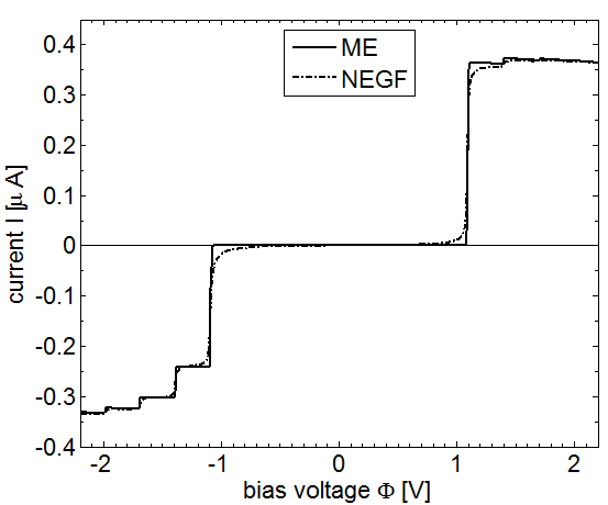
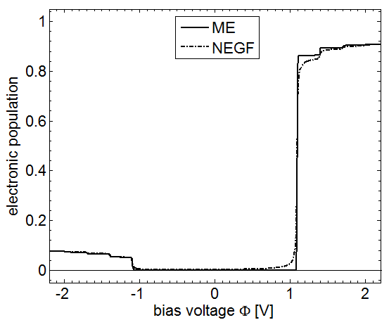
Figure 1: Upper Panel: Current-voltage characteristics for a model molecular junction comprising a single electronic state that is coupled to a single vibrational mode and asymmetrically to a left and a right lead. The solid black line is obtained with the ME approach, while for the dashed black line NEGF is used. Lower Panel: The corresponding population of the electronic state as a function of the applied bias voltage $\Phi$. The asymmetry of the population characteristics with respect to the polarity of the bias voltage is a result of the asymmetric molecule-lead coupling. Electronic-vibrational coupling translates this asymmetry also to the respective current-voltage characteristics, which otherwise (i.e. without electronic-vibrational coupling) would be almost anti-symmetric with respect to $\Phi$.

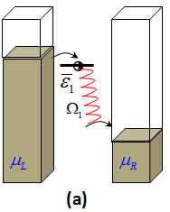
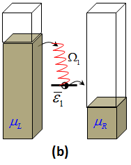
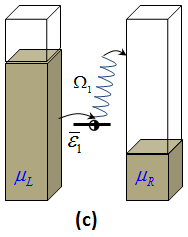
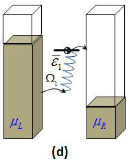
Figure 2: (Color online) Basic schemes of vibrationally coupled electron transport through a single electronic state. Panels a) and b) depict examples for emission processes, where an electron sequentially tunnels from the left lead onto the molecule and further to the right lead, thereby singly exciting the vibrational mode of the molecular bridge (red wiggly lines). Such emission processes are effectively ’heating’ the junction (local heating). Examples for respective absorption processes are shown in Panel c) and d), where electrons tunnel from the left to the right lead by absorbing a quantum of vibrational energy (blue wiggly line).

In contrast to these electronic observables, the corresponding vibrational excitation number, $\langle c^{\dagger}_{\nu}c_{\nu}\rangle_{\hat{H}}$, increases in a series of distinct steps for both polarities of the bias voltage (see Fig. 3). This finding cannot be solely understood in terms of electron transport processes. Although vibrational excitation is a result of inelastic electron transport processes (cf. Figs. 2a-d), another class of processes, which does not contribute to the current, needs to be considered. Resonant electron-hole pair creation processes Härtle et al. (2010); Härtle and Thoss (2011a, b), such as those depicted by Figs. 4a and 4b, are effectively cooling the vibrational mode and diminish the current-induced vibrational excitation. Since these processes involve two sequential tunneling events, they occur with the same probability as respective transport processes. Due to the asymmetry in the molecule-lead coupling, electron-hole pair creation processes with respect to the left lead are the most important ones. They are typically more effective the less vibrational quanta are involved. For this particular model system, cooling by electron-hole pair creation is therefore more pronounced for positive bias voltages, $\Phi>2\bar{\epsilon}_{1}$, where e.g. an electron-hole pair in the left lead can be produced by absorption of just a single quantum of vibrational energy. For negative bias voltages, $\Phi<-2\bar{\epsilon}_{1}$, the creation of an electron-hole pair in the left lead requires the absorption of more than ten vibrational quanta. As a result, vibrational excitation is much smaller for positive bias voltages than for negative ones. Increasing the bias voltage, these pair creation processes are blocked one by one, as the energy gap between the molecular level and the electrode chemical potential increases. The steps in the vibrational excitation characteristics thus become larger with increasing bias voltage due to less efficient cooling by electron-hole pair creation processes Härtle and Thoss (2011a, b). This blocking of pair creation processes appears for both polarities of the bias voltage.

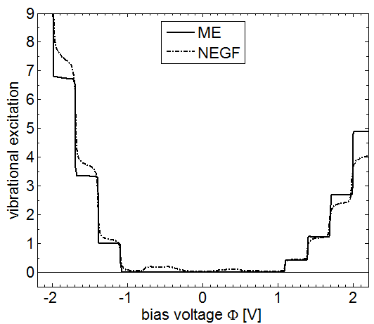
Figure 3: (Color online) Vibrational excitation characteristics corresponding to the current-voltage and population characteristics shown in Fig. 1. Due to the asymmetry in the molecule-lead coupling of this model molecular junction, electron-hole pair creation processes are cooling the vibrational mode more efficiently for positive bias voltages than for negative ones, leading to a strongly asymmetric excitation characteristics. The external bias voltage thus can be used to control the level of vibrational excitation in this asymmetric molecular junction.

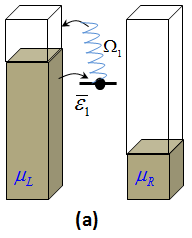
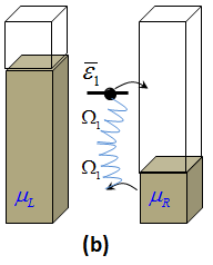
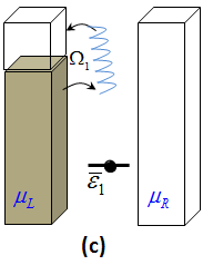
Figure 4: (Color online) Example electron-hole pair creation processes in a molecular junction. Panel a) depicts an electron-hole pair creation process with respect to the left lead by absorption of a single vibrational quantum. Panel b) represents an electron-hole pair creation process with respect to the right lead by absorption of two vibrational quanta. The absorption of two vibrational quanta typically occurs with lower probability. Panel c) shows an off-resonant electron-hole pair creation process.

Apart from the broadening of steps, the ME and the NEGF approach give almost the same vibrational excitation characteristics. However, NEGF can be expected to give slightly larger values for the vibrational excitation, because inelastic co-tunneling processes Lüffe et al. (2008); Härtle et al. (2008, 2009); Leijnse and Wegewijs (2008), which are not included in the ME scheme, additionally contribute to the level of excitation for the vibrational mode. This is particularly important in the off-resonant transport regime, i.e. for $|\Phi|<\bar{\epsilon}_{1}$, where NEGF gives a small vibrational excitation while ME does not. Significant deviations between both approaches occur only for large bias voltages. Especially for large positive bias voltages, e.g. at $\Phi>2$ V, the vibrational excitation obtained from NEGF is significantly smaller than the one obtained by the ME scheme. We attribute this behavior to the contribution of cooling by off-resonant electron-hole pair creation processes, which are missing in the ME approach (an example of an off-resonant pair creation process is depicted in Fig. 4c). These processes become the dominant cooling mechanism at large bias voltages, where resonant electron-hole pair creation processes are suppressed, as they require increasingly higher vibrational energy. In contrast, off-resonant pair creation processes can occur by the absorption of just a single quantum of vibrational energy for all bias voltages. The ME approach thus gives a somewhat larger vibrational excitation than the NEGF method for bias voltages, where resonant electron-hole pair creation processes are strongly suppressed.

The importance of cooling by electron-hole pair creation processes can be corroborated by studying the behavior of the vibrational excitation characteristics with respect to the energy of the electronic state, which for a given bias voltage influences the efficiency of resonant electron-hole pair creation processes. Fig. 5a shows results for the vibrational excitation as a function of the energy $\epsilon_{1}$ at a fixed bias voltage. Thereby, the blue lines refer to a fixed bias voltage of $\Phi=-2$ V, and the red lines to $\Phi=2$ V. As before, solid (dashed) lines refer to calculations performed with the ME (NEGF) scheme. If the energy of the electronic state is closer to the Fermi-level of the system, $\bar{\epsilon}_{1}\to 0$, resonant electron-hole pair creation processes are more strongly suppressed, as they require the absorption of an increasing number of vibrational quanta. The less efficient cooling by resonant electron-hole pair creation leads to the general observed trend of an increasing vibrational excitation with a decreasing energy of the electronic state (for example from $\epsilon_{1}=1$ eV to $\epsilon_{1}=0.4$ eV). For $\epsilon_{1}<0.4$ eV, the NEGF scheme gives a significantly smaller vibrational excitation than the ME method. Here, cooling by off-resonant electron-hole pair creation processes (missing in the ME treatment) results in a significantly lower level of vibrational excitation. Notice that for an asymmetric junction, the value of $\bar{\epsilon}_{1}$ for which the vibrational excitation obtains its maximal value differs from zero and depends on the bias polarity. Considering, e.g. the negative bias voltage (blue lines), a maximum of vibrational excitation is obtained at $\bar{\epsilon_{1}}\sim 0.3$ eV ($\epsilon_{1}\sim 0.35$ eV). For this bias, shifting the electronic level to lower values enhances cooling at the left electrode and suppresses cooling at the right electrode. Due to the asymmetry in the molecule-lead coupling, pair creation processes with respect to the left lead are more important than with respect to the right lead. A minimum of cooling efficiency by electron-hole pair creation processes, which corresponds to a maximum in vibrational excitation, is thus reached for positive values of $\bar{\epsilon}_{1}$. Similarly, for positive bias, a maximum in vibrational excitation appears for negative values of $\bar{\epsilon}_{1}$. Fig. 5b represents the ratio $\langle c_{1}^{\dagger}c_{1}\rangle_{\Phi=-2\text{\,V}}/\langle c_{1}^{\dagger}c_{1}\rangle_{\Phi=+2\text{\,V}}$. It shows that the asymmetry in the vibrational excitation characteristics, as well as in the current-voltage characteristics and the electronic population (data not shown), disappears, once the electronic level is located close to the Fermi-level of the system. This demonstrates that for an electronic state close to the Fermi-level, which can be controlled for example by a gate electrode Sapmaz et al. (2005); Song et al. (2009); Osorio et al. (2010); Martin et al. (2010), the efficiency of both current-induced heating and cooling by electron-hole pair creation processes is the same for both polarities of the bias voltage $\Phi$.

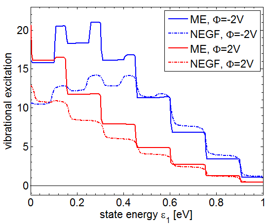
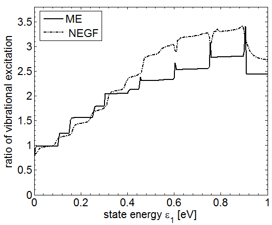
Figure 5: (Color online) Upper Panel: Vibrational excitation as a function of the energy, $\epsilon_{1}$, for a molecular junction with an electronic state coupled to a single vibrational mode and asymmetrically to the leads. Red and blue lines refer to results that are obtained for a fixed bias voltage, $\Phi=\pm 2$ V, respectively. Lower Panel: Ratio of the average vibrational excitation numbers $\langle c_{1}^{\dagger}c_{1}\rangle_{\Phi=-2\text{\,V}}/\langle c_{1}^{\dagger}c_{1}\rangle_{\Phi=+2\text{\,V}}$ shown in the upper panel. The further the electronic level is located from the Fermi-level of the system, which can be controlled for example by a gate electrode, the more pronounced is the asymmetry in vibrational excitation for the different polarities of the bias voltage $\Phi$.

At this point, it is interesting to study the extent of vibrational excitation for different ratios of the molecule-lead couplings $\upsilon_{\text{R},1}/\upsilon_{\text{L},1}$. In Fig. 6, we show the level of excitation of the vibrational mode as a function of the ratio $\upsilon_{\text{R},1}/\upsilon_{\text{L},1}$, where $\upsilon_{\text{L},1}=0.1$ eV is fixed. Again, red and blue lines refer to calculations performed at a fixed bias voltage of $\Phi=\pm 2$ V, respectively. Trivially, for a symmetric junction with $\upsilon_{\text{R},1}=\upsilon_{\text{L},1}$, we obtain the same level of vibrational excitation for both polarities of the bias voltage. Decreasing the coupling to the right lead, the asymmetry in vibrational excitation increases almost linearly. Interestingly, for negative bias voltages, the vibrational excitation obtained by the NEGF scheme (dashed blue line) and by the ME method (solid blue line) approach one another upon decreasing $\upsilon_{\text{R},1}$. This points to the fact that off-resonant electron-hole pair creation processes with respect to the right lead become strongly suppressed. For even smaller coupling strengths to the right lead, $\upsilon_{\text{R},1}<0.03$ eV, the turnover in the dashed blue line (NEGF scheme) indicates that in the limit $\upsilon_{\text{R},1}\rightarrow 0$ current-induced vibrational excitation vanishes, as does the corresponding current. The solid blue line (ME scheme) exhibits the same turn-over but for even smaller coupling strengths to the right lead. On the other hand, for $\Phi=2$ V, the dashed and solid red lines remain well separated upon decreasing the coupling to the right lead, as the ratio between resonant and off-resonant pair creation processes with respect to the left lead remains constant.

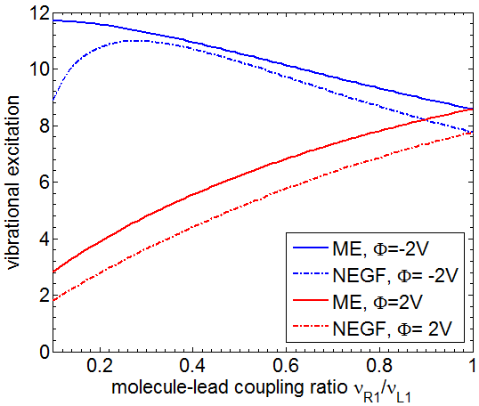
Figure 6: (Color online) Vibrational excitation of a molecular junction with a single electronic state coupled to a single vibrational mode for different coupling strengths to the right lead, $\upsilon_{\text{R},1}$. Thereby, the coupling to the left lead is fixed, $\upsilon_{\text{L},1}=0.1$ eV, as is the bias voltage, $\Phi=\pm 2$ V, for the red and the blue lines, respectively. Asymmetric coupling to the leads facilitates the control of vibrational excitation by the polarity of an external bias voltage.

So far, we have discussed cooling mechanisms for the vibrational mode, which are solely induced by electronic-vibrational coupling. Other vibrational energy relaxation processes, which can be of relevance in molecular junctions, include Intramolecular Vibrational Energy Redistribution processes (IVR) or energy transfer to the environment (e.g. phononic excitation of the electrodes) Segal et al. (2000); Lehmann et al. (2004); May and Kühn (2006); Tao (2006); Jorn and Seidemann (2009). Such relaxation mechanisms are commonly described by coupling of the primary vibrational mode(s) to a thermal heat bath. Fig. 7 shows the level of vibrational excitation as a function of the mode-bath coupling strength $\zeta_{1}$ for a fixed bias voltage (blue lines correspond to $\Phi=-2$ V, and red lines to $\Phi=+2$ V). Naturally, the molecular junction responds to an increased coupling to a ”cold” thermal bath by decreased levels of current-induced vibrational excitation. However, as can be seen by inspection of Eqs. (II.3), vibrational excitation is not only a result of inelastic transport processes, but also stems from the population of the electronic states, that is the formation of a polaronic state Wang and Thoss (2011). Such polaron-formation leads to a finite vibrational excitation even in the limit of strong mode-bath coupling $\zeta_{1}$. Since the electronic level is almost fully populated for positive, but almost unoccupied for negative bias voltages, one observes a higher vibrational excitation for positive bias voltages than for negative bias voltages, if the mode-bath coupling strength $\zeta_{1}$ exceeds a value of $0.02$ eV.

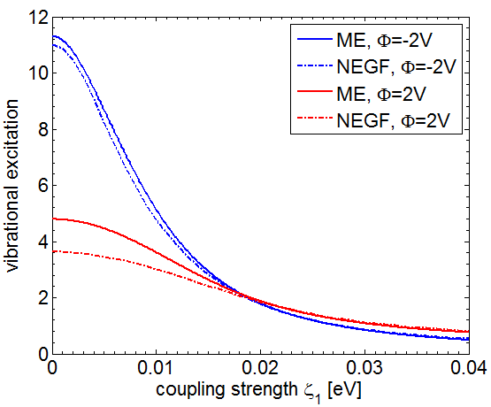
Figure 7: (Color online) Vibrational excitation as a function of the mode-bath coupling strength, $\zeta_{1}$, for a molecular junction with an electronic state coupled to a single vibrational mode and asymmetrically to the leads. Red and blue lines refer to results that are obtained for a fixed bias voltage, $\Phi=\pm 2$ V, respectively. For a strong coupling between the vibrational mode and the thermal bath, vibrational excitation is governed by the formation of a polaronic state.

We finally conclude that in an asymmetric molecular junction the level of vibrational excitation can be controlled by the magnitude and the polarity of the applied bias voltage. It is noted that a gate voltage, which allows to align the energy of electronic states, $\epsilon_{i}$, with respect to the Fermi-level, may facilitate a control mechanism for the ratio between the different levels of vibrational excitation at different bias polarities.

III.2 Mode-Selective Vibrational Excitation

In Sec. III.1 we have outlined how the level of excitation of a single vibrational mode can be controlled by an external bias voltage $\Phi$. In this section, we extend this concept to selective excitation of specific vibrational modes in a junction with multiple vibrational degrees of freedom. In particular, we show that modes with higher frequencies can be stronger excited than low-frequency modes, which corresponds to a ”non-statistical” distribution of vibrational energy. A minimal model for two vibrational modes (model A), which demonstrates such mode-selective vibrational excitation, was recently introduced Härtle et al. (2010). It involves two electronic states, where each state is coupled to one of the vibrational modes and asymmetrically to the leads. Thereby, the asymmetry in the coupling to the leads reflects an inherent asymmetry of the contacted molecule. In this section, we review and extend our earlier study of model A, taking into account intra-molecular correlations, in particular off-diagonal electronic-vibrational coupling, $\lambda_{\nu,m}\neq\delta_{\nu m}$, and electron-electron interactions, $U_{m,n}\neq 0$. Moreover, we consider a different generic realization of an asymmetric molecular junction exhibiting MSVE, model B. Model B also comprises two vibrational modes and two electronic states, asymmetrically coupled to leads, but in contrast to model A, the asymmetry in the molecule-lead coupling is not a result of an intrinsic asymmetry of the molecule, but rather stems from an asymmetry in the electrodes. This corresponds for example to an STM setup, where the molecule bridging the gap between the two electrodes is typically much stronger coupled to the substrate than to the STM tip. These two scenarios, where MSVE can be controlled by an external bias voltage, are schematically depicted in Fig. 8. Respective model parameters are detailed in Table 2. Note that an asymmetric molecule-lead as well as electronic-vibrational coupling is necessary to observe MSVE in both model systems (cf. the discussion of Fig. 6).

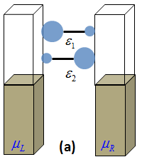
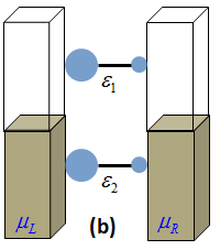
Figure 8: (Color online) Two generic model systems for a molecular junction exhibiting MSVE. Panel (a) depicts a molecular junction, where two electronic states are located above the Fermi-level of the junction, while panel (b) shows a molecular junction that involves an electronic state above and another state below the Fermi-level. Strong (weak) coupling of the electronic states to the leads is represented by large (small) blue dots.

Table 2: Model Parameters (Energy values are given in eV, $K\in\{\text{L,R}\}$, $\alpha\in\{\text{1,2}\}$)

	$\epsilon_{1},\epsilon_{2}$	$\upsilon_{\text{L},1},\upsilon_{\text{L},2}$	$\upsilon_{\text{R},1},\upsilon_{\text{R},2}$	$\xi$	$\gamma$	$\Gamma_{K}(\mu_{K})$	$\omega_{c,\alpha}$	$k_{\text{B}}T$	$\Omega_{1},\Omega_{2}$	$\lambda_{1,1},\lambda_{2,2}$	$\alpha$	$U_{1,2}$	$\zeta_{\alpha}$
Fig. 9	0.65,0.575	0.1,0.03	0.03,0.1	1	2	0.01	1	0.001	0.15,0.2	0.09,0.12	0	0	0
Fig. 10	0.65,0.575	0.1,0.03	0.03,0.1	1	2	0.01	1	0.001	0.15,0.2	0.09,0.12	0	0	0
Fig. 11	0.65,-0.5	0.1,0.1	0.03,0.03	1	2	0.01	1	0.001	0.15,0.2	0.09,0.12	0	0	0
Fig. 12	0.65,-0.5	0.1,0.1	0.03,0.03	1	2	0.01	1	0.001	0.15,0.2	0.09,0.12	0	0	0
Fig. 13	0.65,0.575	0.1,0.03	0.03,0.1	1	2	0.01	1	0.001	0.15,0.2	0.09,0.12	0 – 1	0	0
Fig. 14	0.65,-0.5	0.1,0.1	0.03,0.03	1	2	0.01	1	0.001	0.15,0.2	0.09,0.12	0 – 1	0	0
Fig. 16	0.65,0.575	0.1,0.03	0.03,0.1	1	2	0.01	1	0.001	0.15,0.2	0.09,0.12	0	0 – 1.5	0
Fig. 17	0.65,-0.5	0.1,0.1	0.03,0.03	1	2	0.01	1	0.001	0.15,0.2	0.09,0.12	0	0 – 1.5	0

III.2.1 The Basic Phenomenon

First, we discuss results, where we do not account for a coupling between the vibrational modes and a thermal bath ($\zeta_{1}=\zeta_{2}=0$), nor for off-diagonal electronic-vibrational coupling ($\lambda_{\nu,m}\sim\delta_{\nu,m}$) or electron-electron interactions ($U_{1,2}=0$). Current-voltage characteristics and the corresponding population of the electronic states are shown in Figs. 9 and 11 for model A and B, respectively. The corresponding levels of vibrational excitation are depicted in Figs. 10 and 12. In both models, the excitation of the two normal modes is calculated with respect to the neutral molecule, in which the two electronic states (LUMO and LUMO+1) are unoccupied. Notice, however, that while in model A these states become occupied only for non-zero bias, in model B the molecule (LUMO) is charged (and therefore to some extent vibrationally excited) already at zero bias. Since $\lambda_{\nu,m}\propto\delta_{\nu,m}$ and $U_{1,2}=0$, the two subsystems, the one comprising state 1 and mode 1, and the other consisting of state 2 and mode 2, are interrelated only by the coupling of the two electronic states to the leads. This coupling, however, does not induce strong correlations between the two subsystems, because the electronic states are non-degenerate, i.e., $|\epsilon_{2}-\epsilon_{1}|>\Gamma$. The transport characteristics of model A and B can therefore, in principle, be understood by the arguments given in Sec. III.1 for a single electronic state and a single vibrational mode. In particular, the agreement of the results obtained with NEGF and ME, which we already found in Sec. III.1, is maintained.

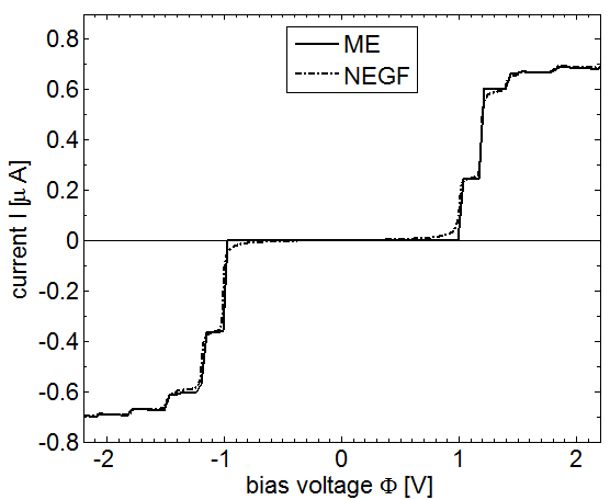
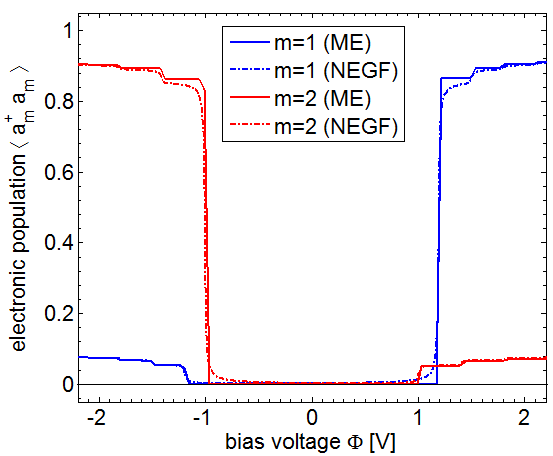
Figure 9: (Color online) Current-voltage characteristics and the respective population of the electronic states for the model system depicted by Fig. 8a (model A). Solid (dashed dotted) lines are obtained employing the ME (NEGF) methodology. The population characteristics of state 1 and 2 are depicted by the blue and the red line, respectively. While the current is almost anti-symmetric with respect to the bias voltage $\Phi$, the population of the electronic levels reflects the asymmetry in the coupling of the two states to the left and the right lead.

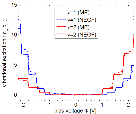
Figure 10: (Color online) Average levels of vibrational excitation for the two modes in model A as a function of the applied bias voltage $\Phi$. The blue and the red line depict the excitation characteristics of mode 1 and mode 2, respectively. Despite the different frequencies of the modes, mode 1 is much higher excited than mode 2 for negative bias voltages, while it is less excited than mode 2 for positive bias voltages. The excitation of the two modes can thus be selectively controlled by the external bias voltage $\Phi$ (MSVE).

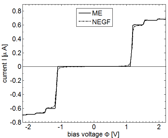
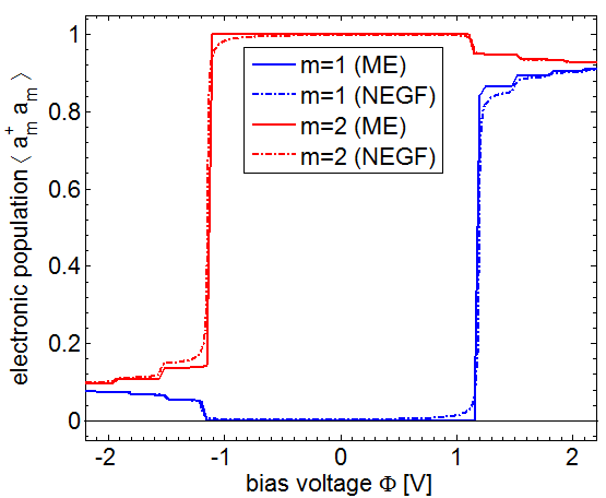
Figure 11: (Color online) Current-voltage characteristics and the respective population the electronic states for the model system depicted by Fig. 8b (model B). Solid (dashed dotted) lines are obtained employing the ME (NEGF) methodology. The population characteristics of state 1 and 2 are depicted by the blue and the red line, respectively. While the current is almost anti-symmetric with respect to the bias voltage $\Phi$, the population of the electronic levels reflects the asymmetry in the coupling of the molecule to the left and the right lead.

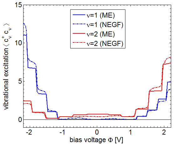
Figure 12: (Color online) Average levels of vibrational excitation for the two modes in model B as a function of the applied bias voltage $\Phi$. The blue and the red line depict the excitation characteristics of mode 1 and mode 2, respectively. Despite the different frequencies of the two modes, mode 1 is much higher excited than mode 2 for negative bias voltages, while it is less excited than mode 2 for positive bias voltages. The excitation of the two modes can thus be selectively controlled by the external bias voltage $\Phi$ (MSVE).

While for both models the current-voltage characteristics is almost anti-symmetric with respect to the applied bias voltage $\Phi$, the electronic population and average levels of vibrational excitation exhibit strong asymmetric behavior. In particular, for negative bias voltages mode 1 shows a much higher level of vibrational excitation than mode 2. For positive bias voltages, however, the distribution of vibrational energy is reversed and mode 2 is higher excited than mode 1, despite the fact that $\Omega_{2}>\Omega_{1}$.

These results, where no intra-molecular interactions are considered, are in line with the interpretation and the analysis for cooling of vibrational modes by electron-hole pair creation processes (cf. Sec. III.1). In particular, it is sufficient to consider the asymmetry in the coupling of each electronic state to the two leads, and the energy gap between each electronic state and the chemical potential of the two electrodes in order to assess which of the two vibrations is more effectively excited. In a realistic model of a molecular junction, however, correlations need to be taken into account. To this end, we analyze MSVE in the next three sections in terms of off-diagonal electronic-vibrational coupling, $\lambda_{\nu,m}\neq\delta_{\nu,m}$, electron-electron interactions, $U_{1,2}\neq 0$, and in the presence of efficient cooling by coupling to a cold nuclear bath, $\zeta_{1}\neq 0$ and $\zeta_{2}\neq 0$.

III.2.2 MSVE in the Presence of Off-Diagonal Electronic-Vibrational Coupling

As shown above, the MSVE phenomenon depends predominantly on the efficiency of cooling by electron-hole pair creation processes. This efficiency can be selectively controlled by the external bias voltage due to the asymmetry not only in the molecule-lead coupling, but also in the electronic-vibrational coupling. The latter is most pronounced when each mode is coupled exclusively to a different electronic state, i.e., $\lambda_{\nu,m}\sim\delta_{\nu,m}$. In Figs. 13 and 14, for model A and B, respectively, the vibrational excitation of the two modes is shown for increasing off-diagonal electronic-vibrational coupling: $\lambda_{1,2}=\alpha\lambda_{1,1}$ and $\lambda_{2,1}=\alpha\lambda_{2,2}$, where $\alpha=0$ describes the absence of off-diagonal vibronic coupling, while for $\alpha=1$ off-diagonal coupling is as strong as the diagonal one. Thereby, we use a fixed bias voltage $\Phi=+2$ V for Figs. 13a and 14a, and $\Phi=-2$ V for Figs. 13b and 14b. The results demonstrate that off-diagonal electronic-vibrational coupling tends to decrease MSVE for these model molecular junctions, as might have been anticipated. MSVE, however, remains significant for a broad range of coupling strengths $\alpha$. A more detailed analysis rationalizes the trends in each case.

In model A, at positive bias (Fig. 13a) and for $\alpha=0$, cooling by electron-hole pair creation is more effective via the state that is coupled more strongly to the left electrode (state 1). Therefore, the mode coupled to this state, that is mode 1, is more effectively cooled. As $\alpha$ increases, mode 2 becomes coupled to state 1, and cooling by electron-hole pair creation becomes effective also for this mode. While the level of excitation of mode 1 is thus almost the same for all values of $\alpha$, the one of mode 2 decreases. Similar arguments hold for negative bias voltages (Fig. 13b), where electron-hole pair creation via state 2 at the right electrode is the dominant cooling mechanism.
Notice that off-diagonal coupling also involves a change in the nuclear reorganization energy of each electronic state. This is particularly pronounced for transport and pair creation processes involving the di-anionic states (or a doubly occupied molecular bridge, cf. Fig. 15), which reorganization energies also involve vibrationally induced electron-electron interactions ($\bar{U}_{1,2}\approx 0.25$ eV for $\alpha=1$, see Sec. II.3). Since state 1 (2) is almost fully occupied for $\Phi=2$ V ($\Phi=-2$ V), processes involving state 2 (1) are dominated by the di-anionic resonance at $\bar{\epsilon}_{2(1)}+\bar{U}_{1,2}$. Increasing $\alpha$ shifts this resonance to significantly lower energies. This shift manifests itself in the kink observed in the vibrational excitation of mode 2 (1) at $\alpha=0.4$ for $\Phi=2$ V (at $\alpha=0.2$ for $\Phi=-2$ V), indicating the suppression of electron-hole pair creation processes (cf. Fig. 15a) as the respective resonance is shifted further away from the chemical potential in the left (right) electrode. Note that such kinks are less pronounced for larger values of $\alpha$, where cooling by electron-hole pair creation processes occurs for each mode via both electronic states such that the closure of one of these cooling channels is less significant.

Similar trends are observed for model B (cf. Fig. 14). For negative bias and $\alpha=0$, mode 2 is more effectively cooled due to the strong coupling between state 2 and the left electrode. Increasing $\alpha$, mode 1 becomes coupled to that state as well, leading to a suppression of vibrational excitation also for this mode. Notice that di-anionic resonances are less important in this case as the two states are almost unoccupied. Therefore, kinks associated with the reorganization energy of the electronic levels are also less pronounced. For positive bias, however, the two electronic states are almost fully occupied, and therefore, transport and pair creation processes do occur predominantly by the di-anionic resonances. Since these resonances are shifted to lower energies with increasing $\alpha$, state 1 is effectively located further away from the chemical potential in the left electrode and state 2 closer to the one in the right electrode. This results in less (more) efficient cooling by electron-hole pair creation processes, and respectively, in an increased (decreased) level of vibrational excitation. The latter trends bring the excitation levels of the two modes to similar values already for $\alpha\approx 0.2-0.5$, which suppresses MSVE for this model. We note however, that the ’Coulomb-like’ attraction term ($\bar{U}$), which dominates the suppression of MSVE, is typically compensated by repulsive electron-electron interactions, which, however, are not accounted for in the present model.

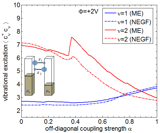
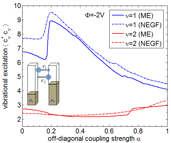
Figure 13: (Color online) Average vibrational excitation of the two vibrational modes in model A as a function of the off-diagonal electronic-vibrational coupling strength $\alpha$. The top and the bottom plots correspond to a fixed bias voltage of $\Phi=\pm 2$ V, respectively, as illustrated in the insets. Although off-diagonal electronic-vibrational coupling distributes current-induced excitation among the vibrational modes, MSVE occurs for a broad range of coupling strengths $\alpha$.

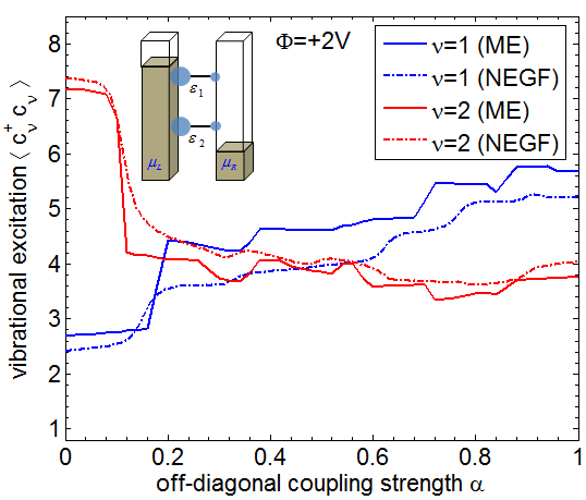
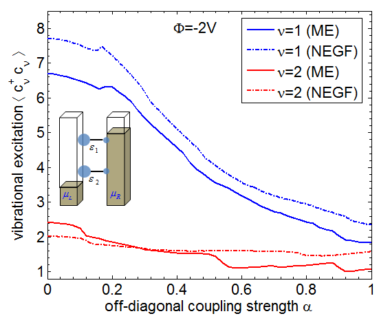
Figure 14: (Color online) Average vibrational excitation of the two vibrational modes in model B as a function of the off-diagonal electronic-vibrational coupling strength $\alpha$. The top and the bottom plots correspond to a fixed bias voltage of $\Phi=\pm 2$ V, respectively, as illustrated in the insets. Although off-diagonal electronic-vibrational coupling distributes current-induced excitation among the vibrational modes, MSVE occurs for a broad range of coupling strengths $\alpha$.

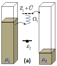
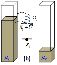
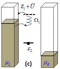
Figure 15: (Color online) Schematic representation of Coulomb-assisted transport processes (Panel (a)) and Coulomb-assisted electron-hole pair creation processes (Panels (b) and (c)). The dashed line represents the position of the di-anionic (doubly occupied) resonance, where state 2 is considered occupied. Similar processes are available at energies $\bar{\epsilon}_{2}+\bar{U}$. The position of the two electronic states with respect to the chemical potentials in the left and the right lead, $\bar{\epsilon}_{1/2}-\mu_{\text{L/R}}$, and the positions of the di-anionic resonances, $\bar{\epsilon}_{1/2}+\bar{U}-\mu_{\text{L/R}}$, determine the efficiency of heating and cooling processes.

III.2.3 MSVE in the Presence of Electron-Electron Interactions

A comparison of the electronic populations, shown in Figs. 9b and 11b, and the associated levels of vibrational excitation, given in Figs. 10 and 12, shows that these quantities are strongly correlated. Electron-electron interactions, $U_{m,n}\neq 0$, can strongly influence the electronic population of the different states Hettler et al. (2002, 2003); Muralidharan and Datta (2007); Härtle and Thoss (2011a); Leijnse et al. (2011) and thus the degree of MSVE in an asymmetric molecular junction. We study the effect of such inter-state correlations on MSVE in Figs. 16 and 17, where the levels of excitation for the two vibrational modes in model A and B are plotted as functions of the electron-electron interaction strength $U_{1,2}=U$, using fixed bias voltages $\Phi=\pm 2$ V.

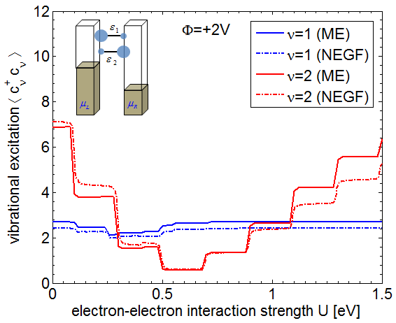
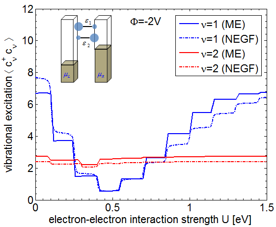
Figure 16: (Color online) Vibrational excitation as a function of the electronic interaction strength $U$ in model A. Blue (red) lines refer to the average excitation number of mode 1 (2). The top and the bottom plots correspond to a fixed bias voltage of $\Phi=\pm 2$ V, respectively. The efficiency of cooling mode 2 (1) by electron-hole pair creation processes with respect to the di-anionic (doubly occupied) state varies with the electron-electron interaction strengths $U$ for positive (negative) bias voltages. This leads to a inversion of MSVE for intermediate values of $U$, where the energy of the corresponding di-anionic state, $\bar{\epsilon}_{2}+U$ ($\bar{\epsilon}_{1}+U$), is close to the chemical potential in the left (right) lead.

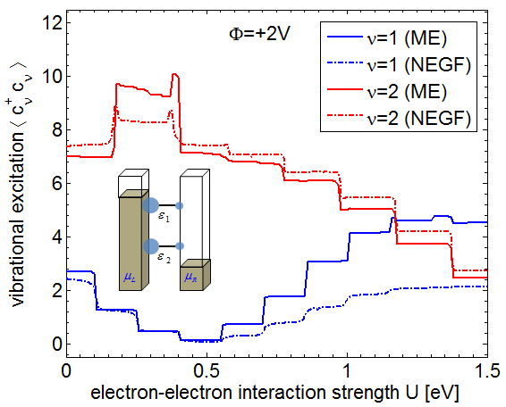
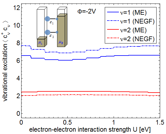
Figure 17: (Color online) Vibrational excitation as a function of the electronic interaction strength $U$ in model B. Blue (red) lines refer to the average excitation number of mode 1 (2). The top and the bottom plots correspond to a fixed bias voltage of $\Phi=\pm 2$ V, respectively. For negative bias voltages, due to the weak coupling to the right lead, both states are more or less unpopulated, which translates to a weak dependence of vibrational excitation on $U$. For positive bias voltages, however, double occupancy of the molecular bridge becomes important, and thus, the specific levels of vibrational excitation show a strong dependence on $U$. While MSVE thus exhibits a strong enhancement for weak and intermediate electron-electron interactions strengths, it is attenuated for higher values of $U$.

In model A (Fig. 16), the dependence of the two vibrational mode-excitations on $U$ is nearly reversed when the bias is reversed, demonstrating MSVE for most values of $U$. The particular levels of vibrational excitation and the direction of MSVE reflect the detailed asymmetry of the molecular junction. For example, for $\Phi=2$ V the excitation of mode 1 is nearly independent on $U$, while the one of mode 2 shows a strong non-monotonic dependence. Since mode 1 is coupled to state 1, and because state 2 is almost unoccupied in this regime, mode 1 is efficiently cooled by electron-hole pair creation processes with respect to the left electrode, regardless of the electron-electron interaction strength $U$. In contrast, mode 2 is coupled to state 2 that is only weakly coupled to the left lead, and therefore, not efficiently cooled by electron-hole pair creation processes for $U=0$. However, as $U$ increases, electron tunneling with respect to state 2 involves an increasingly larger charging energy, $\bar{\epsilon}_{2}+U$, since state 1 is almost fully occupied. This brings the electronic energy in this transport channel first closer to and then further away from the chemical potential in the left electrode. Cooling of mode 2 by electron-hole pair creation processes (Coulomb-assisted electron-hole pair creation processes as depicted in Figs. 15b and 15c) is thus first enhanced and then suppressed as $U$ increases, resulting in the observed non-monotonic level of vibrational excitation. Notice that the pronounced cooling due to Coulomb-assisted electron-hole pair creation processes, in the intermediate regime of electron-electron interaction strengths, $U$, reverses the direction of MSVE with respect to the $U=0$ case (cf. Fig. 16).

In model B (Fig. 17) the asymmetry in the coupling of the molecular bridge to the electrodes leads to very different dependencies of the vibrational mode-excitations on $U$ for different polarities of the applied bias voltage. The resulting dependence of MSVE on $U$ is non-trivial, ranging from enhancement to suppression of the effect with respect to $U=0$. At negative bias voltages the two electronic states remain nearly unoccupied, so that the effect of electron-electron interactions is negligible. The lower excitation level of mode 2 at this polarity of the bias voltage reflects more efficient cooling by electron-hole pair creation via state 2 at the left electrode (Fig. 17), which is maintained for different values of $U$. For positive bias voltages, the two electronic states are almost fully occupied. Cooling of mode 1 and 2 is thus dominated by electron-hole pair creation at the left and the right leads, respectively, according to the proximity of the corresponding energy levels, $\bar{\epsilon}_{1}+U$ and $\bar{\epsilon}_{2}+U$, to the respective chemical potentials. As $U$ increases, electron-hole pair creation at the left electrode is enhanced, while pair creation with respect to the right lead is suppressed. This leads first to an enhancement of MSVE with respect to $U=0$. At $U\approx 0.4$ eV, however, the electronic energy $\bar{\epsilon}_{1}+U$ crosses the chemical potential in the left lead, and state 1 becomes discharged. At this point, cooling of mode 1 is at its maximal efficiency. Simultaneously, since state 1 is no longer populated ($\langle a_{1}^{\dagger}a_{1}\rangle$ drops from $\approx 0.9$ to $\approx 0.1$), processes involving state 2 occur predominantly via the anionic channel at $\bar{\epsilon}_{2}$, such that cooling of mode 2 by electron-hole pair creation processes with respect to the right electrode becomes as efficient as for $U=0$. Accordingly, the level of excitation for mode 2 returns to its original value. Increasing $U$ even further cooling of mode 1 (via the di-anionic channel, $\bar{\epsilon}_{1}+U$) becomes less efficient, and the level of excitation for mode 1 increases again. As $\bar{\epsilon}_{2}+U$ is closer to the chemical potential in the left lead, the cooling efficiency of mode 2 by electron-hole pair creation processes with respect to the left lead increases. The overall effect leads to a suppression of MSVE for $U\gtrsim 1$ eV in the given range of electron-electron interactions strengths $U$. Note, however, that for yet larger values of the electron-electron interaction strength, $U\gtrsim 2.5$ eV, MSVE is regained and becomes approximately as pronounced as for $U=0$. In this regime, transport and pair creation processes are dominated by the anionic resonances (at $\bar{\epsilon}_{1/2}$) so that the asymmetry in the cooling efficiency of the two modes (at least for the present model) is the same as for $U=0$.

III.2.4 MSVE for Strong Vibrational Relaxation

In the discussion of Fig. 7 in Sec. III.1, we have already seen that the level of excitation of a single vibrational mode consists of two contributions: current-induced local heating due to inelastic electron transport processes (as shown in Figs. 2a-d), and polaron-formation Wang and Thoss (2011), which can be quantified by the difference

$$\langle c_{\nu}^{\dagger}c_{\nu}\rangle_{\hat{H}}-\langle c_{\nu}^{\dagger}c_{\nu}\rangle_{\bar{H}}=\sum_{mm^{\prime}}(\lambda_{\nu,m}\lambda_{\nu,m^{\prime}}/\Omega_{\nu}^{2})\langle a_{m}^{\dagger}a_{m}a_{m^{\prime}}^{\dagger}a_{m^{\prime}}\rangle_{\bar{H}}.$$ (58)

Strong vibrational relaxation results in a strong suppression of current-induced vibrational excitation, especially if the time-scale for vibrational relaxation is much shorter than the time-scale between two consecutive transport events. The contribution due to polaron formation, however, stems from the steady-state population of the electronic levels in a molecular junction. Hence, for model A, MSVE occurs in the presence of strong vibrational relaxation Härtle et al. (2010), since the population of the electronic levels can be selectively controlled by the external bias voltage $\Phi$ (cf. Fig. 9b). In model B, however, both states are either fully populated or empty such that strong vibrational relaxation is likely to hinder MSVE for this model system.

IV Conclusion

In this work we have studied and analyzed transport characteristics of single-molecule junctions, focusing on the excitation of specific molecular vibrational modes. In particular, we have shown that the level of excitation of specific modes can be controlled by the polarity and the magnitude of an external bias voltage. Thereby, high-frequency modes (typically associated with strong chemical bonds) can be higher excited than low-frequency modes, which translates to a ”non-statistical” distribution of energy among the vibrational modes. We refer to this phenomenon as mode-selective vibrational excitation.

Our main findings are summarized below:

• The importance of cooling by electron-hole pair creation
  Our analysis shows that cooling of the vibrational modes in a molecular junction by electron-hole pair creation processes is crucial to understand the extent of the MSVE phenomenon. In particular, since the efficiency of these processes is sensitive to the position of the chemical potentials in the leads, the levels of vibrational excitation in the molecule can be controlled by an external bias voltage. Considering a molecule with multiple vibrational modes and typical asymmetries in the vibronic as well as molecule-lead couplings, the level of excitation of specific vibrational modes can thus be tuned by the polarity and the magnitude of the external bias voltage.

• The role of asymmetry and intra-molecular interactions
  Our studies suggest that MSVE is a rather general phenomenon and is likely to be observed experimentally. The required asymmetry in the electronic interaction between different molecular states and the leads may be due to an inherent asymmetric molecular structure (model A) or stem from an inherent difference between the two electrodes, as e.g. in STM experiments (model B). Intra-molecular interactions, e.g. due to off diagonal electronic-vibrational coupling or electron-electron repulsion tend to redistribute the excitation energy between the different modes, and thus work against MSVE. However, having analyzed a broad range of parameters, we found the MSVE phenomenon to prevail even in the presence of such interactions.

• The importance of off-resonant processes: Comparing ME to NEGF calculations.
  Our numerical studies of generic models of molecular junctions were based on two complementary theoretical methods: a nonequilibrium Green’s function approach Härtle et al. (2008, 2009, 2010, 2011) and a master equation approach Volkovich et al. (2008); Peskin (2010); Volkovich and Peskin (2011). Both approaches are based on a second-order expansion in the coupling of the molecular bridge to the leads. While the NEGF method also accounts for higher-order effects, the ME approach describes only resonant electron tunneling processes. However, intra-molecular interactions, either due to electronic-vibrational coupling or electron-electron interactions, can be described by the ME method without invoking further approximations, while these interactions are described by our NEGF approach approximately in terms of a non-perturbative scheme. Although the results obtained by both methodologies agree in most cases reasonably well, further insights into the relevant mechanisms can be gained when the results exhibit differences. Thus, for example, the importance of off-resonant electron-hole pair creation processes for local cooling Härtle et al. (2009); Galperin et al. (2009); Schiff and Nitzan (2010); Romano et al. (2010); Härtle and Thoss (2011a) of vibrational modes in the high-bias regime could be revealed.

We end by noting that this work considered only generic models to study the basic mechanisms and prerequisites of bias-controlled MSVE. The identification of specific molecules that exhibit MSVE requires transport studies based on first-principles electronic structure calculations Pecchia and Di Carlo (2004); Frederiksen et al. (2004); Benesch et al. (2006); Troisi and Ratner (2006); Benesch et al. (2006, 2008, 2009); Monturet et al. (2010). This will be the subject of future work. Another interesting extension concerns the external control mechanism for MSVE. In the present work, we have considered an external bias voltage as the means to control MSVE. A gate electrode Sapmaz et al. (2005); Song et al. (2009); Osorio et al. (2010); Martin et al. (2010) may provide another tool for addressing a molecular junction with an electric field, and thus, may also be used to control vibrational excitation. Finally, in the context of mode-selective chemistry, studies of MSVE in single-molecule junctions may pave the way to control chemical processes in molecules adsorbed on surfaces. For example, an additional electrode that provides an external potential bias may induce catalytic reactions in a selective manner.

Acknowledgements:

We gratefully acknowledge fruitful discussions with O. Godsi, D. Brisker Klaiman, M. Butzin, P. Brana-Coto and O. Rubio-Pons. This research was supported by the German-Israeli Foundation for scientific development (GIF). RV acknowledges support from the Gutwirth Foundation. The Leibniz Rechenzentrum Munich (LRZ) and the Regionales Rechenzentrum Erlangen (RRZE) were providing the computer resources for our studies. The work at the Friedrich-Alexander Universität Erlangen-Nürnberg was carried out in the framework of the Cluster of Excellence ”Engineering of Advanced Materials”.

References

- Jortner et al. (1991) J. Jortner, R. D. Levine, and B. Pullman, Mode selective chemistry (Kluwer, Amsterdam, 1991).
- Liu et al. (2006) Z. Liu, L. C. Feldman, N. H. Tolk, Z. Zhang, and P. I. Cohen, Science 312, 1024 (2006).
- Crim (2008) F. F. Crim, Proc. Natl. Acad. Sci. U.S.A. 105, 12654 (2008).
- Potter et al. (1992) E. D. Potter, J. L. Herek, S. Pedersen, Q. Liu, and A. H. Zewail, Nature 355, 66 (1992).
- Zare (1998) R. Zare, Science 279, 1875 (1998).
- Brumer and Shapiro (2003) P. W. Brumer and M. Shapiro, Principles of the Quantum Control of Molecular Processes (Wiley, New Jersey, 2003).
- Bryan et al. (2011) W. A. Bryan, C. R. Calvert, R. B. King, G. R. A. J. Nemeth, J. D. Alexander, J. B. Greenwood, C. A. Froud, I. C. E. Turcu, E. Springate, W. R. Newell, et al., Phys. Rev. A 83, 021406 (2011).
- Joachim and Roth (1997) C. Joachim and S. Roth, Atomic and molecular wires (Kluwer, Dordrecht, 1997).
- Park et al. (2000) H. Park, J. Park, A. K. L. Lim, E. H. Anderson, A. P. Alivisatos, and P. L. McEuen, Nature (London) 407, 57 (2000).
- Reichert et al. (2002) J. Reichert, R. Ochs, D. Beckmann, H. B. Weber, M. Mayor, and H. v. Lohneysen, Phys. Rev. Lett. 88, 176804 (2002).
- Smit et al. (2002) R. Smit, Y. Noat, C. Untiedt, N. Lang, M. van Hemert, and J. van Ruitenbeek, Nature (London) 419, 906 (2002).
- Nitzan and Ratner (2003) A. Nitzan and M. A. Ratner, Science 300, 1384 (2003).
- Pascual et al. (2003) J. I. Pascual, N. Lorente, Z. Song, H. Conrad, and H. P. Rust, Nature 423, 525 (2003).
- Wu et al. (2004) S. W. Wu, G. V. Nazin, X. Chen, X. H. Qiu, and W. Ho, Phys. Rev. Lett. 93, 236802 (2004).
- Ogawa et al. (2007) N. Ogawa, G. Mikaelian, and W. Ho, Phys. Rev. Lett. 98, 166103 (2007).
- Hihath et al. (2008) J. Hihath, C. R. Arroyo, G. Rubio-Bollinger, N. J. Tao, and N. Agrait, Nano Lett. 8, 1673 (2008).
- Schulze et al. (2008) G. Schulze, K. J. Franke, A. Gagliardi, G. Romano, C. S. Lin, A. Da Rosa, T. A. Niehaus, T. Frauenheim, A. Di Carlo, A. Pecchia, et al., Phys. Rev. Lett. 100, 136801 (2008).
- Pump et al. (2008) F. Pump, R. Temirov, O. Neucheva, S. Soubatch, S. Tautz, M. Rohlfing, and G. Cuniberti, Appl. Phys. A 93, 335 (2008).
- Ballmann et al. (2010) S. Ballmann, W. Hieringer, D. Secker, Q. Zheng, J. A. Gladysz, A. Görling, and H. B. Weber, ChemPhysChem 11, 2256 (2010).
- Osorio et al. (2010) E. A. Osorio, M. Ruben, J. S. Seldenthuis, J. M. Lehn, and H. S. J. van der Zant, Small 6, 174 (2010).
- Hihath et al. (2010) J. Hihath, C. Bruot, and N. Tao, ACS Nano 4, 3823 (2010).
- Cuevas and Scheer (2010) J. C. Cuevas and E. Scheer, Molecular Electronics: An Introduction To Theory And Experiment (World Scientific, Singapore, 2010).
- Secker et al. (2011) D. Secker, S. Wagner, S. Ballmann, R. Härtle, M. Thoss, and H. B. Weber, Phys. Rev. Lett. 106, 136807 (2011).
- Yu et al. (2004) L. H. Yu, Z. K. Keane, J. W. Ciszek, L. Cheng, M. P. Stewart, J. M. Tour, and D. Natelson, Phys. Rev. Lett. 93, 266802 (2004).
- Huang et al. (2006) Z. Huang, B. Xu, Y. Chen, M. Di Ventra, and N. Tao, Nano Lett. 6, 1240 (2006).
- Ward et al. (2008) D. R. Ward, N. J. Halas, J. W. Ciszek, J. M. Tour, Y. Wu, P. Nordlander, and D. Natelson, Nano Lett. 8, 919 (2008).
- Repp et al. (2010) J. Repp, P. Liljeroth, and G. Meyer, Nature Physics 6, 975 (2010).
- Mitra et al. (2004) A. Mitra, I. Aleiner, and A. J. Millis, Phys. Rev. B 69, 245302 (2004).
- Koch et al. (2006) J. Koch, M. Semmelhack, F. von Oppen, and A. Nitzan, Phys. Rev. B 73, 155306 (2006).
- Koch and von Oppen (2005) J. Koch and F. von Oppen, Phys. Rev. Lett. 94, 206804 (2005).
- Ioffe et al. (2008) Z. Ioffe, T. Shamai, A. Ophir, G. Noy, I. Yutsis, K. Kfir, O. Cheshnovsky, and Y. Selzer, Nat. Nano. 3, 727 (2008).
- Härtle et al. (2008) R. Härtle, C. Benesch, and M. Thoss, Phys. Rev. B 77, 205314 (2008).
- Härtle et al. (2009) R. Härtle, C. Benesch, and M. Thoss, Phys. Rev. Lett. 102, 146801 (2009).
- Härtle et al. (2010) R. Härtle, R. Volkovich, M. Thoss, and U. Peskin, J. Chem. Phys. 133, 081102 (2010).
- Härtle and Thoss (2011a) R. Härtle and M. Thoss, Phys. Rev. B 83, 115414 (2011a).
- Entin-Wohlman et al. (2010) O. Entin-Wohlman, Y. Imry, and A. Aharony, Phys. Rev. B 81, 113408 (2010).
- Härtle and Thoss (2011b) R. Härtle and M. Thoss, Phys. Rev. B 83, 125419 (2011b).
- Härtle et al. (2011) R. Härtle, M. Butzin, O. Rubio-Pons, and M. Thoss, arXiv:1102.4190 (2011).
- Gaudioso et al. (2000) J. Gaudioso, L. J. Lauhon, and W. Ho, Phys. Rev. Lett. 85, 1918 (2000).
- Choi et al. (2006) B. Y. Choi, S. J. Kahng, S. Kim, H. Kim, H. W. Kim, Y. J. Song, J. Ihm, and Y. Kuk, Phys. Rev. Lett. 96, 156106 (2006).
- Lafferentz et al. (2009) L. Lafferentz, F. Ample, H. Yu, S. Hecht, C. Joachim, L. Grill, and M. A. Reed, Science 27, 1193 (2009).
- May (2002) V. May, Phys. Rev. B 66, 245411 (2002).
- Lehmann et al. (2004) J. Lehmann, S. Kohler, V. May, and P. Hänggi, J. Chem. Phys. 121, 2278 (2004).
- Ovchinnikov and Neuhauser (2005) I. V. Ovchinnikov and D. Neuhauser, J. Chem. Phys. 122, 024707 (2005).
- Pedersen and Wacker (2005) J. N. Pedersen and A. Wacker, Phys. Rev. B 72, 195330 (2005).
- Welack et al. (2006) S. Welack, M. Schreiber, and U. Kleinekathöfer, J. Chem. Phys. 124, 044712 (2006).
- Harbola et al. (2006) U. Harbola, M. Esposito, and S. Mukamel, Phys. Rev. B 74, 235309 (2006).
- Zazunov et al. (2006) A. Zazunov, D. Feinberg, and T. Martin, Phys. Rev. B 73, 115405 (2006).
- Siddiqui et al. (2007) L. Siddiqui, A. W. Ghosh, and S. Datta, Phys. Rev. B 76, 085433 (2007).
- Timm (2008) C. Timm, Phys. Rev. B 77, 195416 (2008).
- May and Kühn (2008a) V. May and O. Kühn, Phys. Rev. B 77, 115439 (2008a).
- May and Kühn (2008b) V. May and O. Kühn, Phys. Rev. B 77, 115440 (2008b).
- Leijnse and Wegewijs (2008) M. Leijnse and M. R. Wegewijs, Phys. Rev. B 78, 235424 (2008).
- Esposito and Galperin (2009) M. Esposito and M. Galperin, Phys. Rev. B 79, 205303 (2009).
- (55) M. Esposito and M. Galperin, J. Phys. Chem. C (????).
- Peskin (2010) U. Peskin, J. Phys. B: At. Mol. Opt. Phys. 43, 153001 (2010).
- Pshenichnyuk and Cizek (2011) I. Pshenichnyuk and M. Cizek, Phys. Rev. B 83, 165446 (2011).
- Volkovich and Peskin (2011) R. Volkovich and U. Peskin, Phys. Rev. B 83, 033403 (2011).
- König et al. (1996) J. König, H. Schoeller, and G. Schön, Phys. Rev. Lett. 76, 1715 (1996).
- Paaske and Flensberg (2005) J. Paaske and K. Flensberg, Phys. Rev. Lett. 94, 176801 (2005).
- Sela et al. (2006) E. Sela, Y. Oreg, F. von Oppen, and J. Koch, Phys. Rev. Lett. 97, 086601 (2006).
- Galperin et al. (2007) M. Galperin, A. Nitzan, and M. A. Ratner, Phys. Rev. B 76, 035301 (2007).
- Lüffe et al. (2008) M. C. Lüffe, J. Koch, and F. von Oppen, Phys. Rev. B 77, 125306 (2008).
- Leijnse et al. (2009) M. Leijnse, M. R. Wegewijs, and M. H. Hettler, Phys. Rev. Lett. 103, 156803 (2009).
- Han (2010) J. E. Han, Phys. Rev. B 81, 113106 (2010).
- Flensberg (2003) K. Flensberg, Phys. Rev. B 68, 205323 (2003).
- Galperin et al. (2006) M. Galperin, A. Nitzan, and M. A. Ratner, Phys. Rev. B 73, 045314 (2006).
- Ryndyk et al. (2006) D. A. Ryndyk, M. Hartung, and G. Cuniberti, Phys. Rev. B 73, 045420 (2006).
- Frederiksen et al. (2007) T. Frederiksen, N. Lorente, M. Paulsson, and M. Brandbyge, Phys. Rev. B 75, 235441 (2007).
- Tahir and MacKinnon (2008) M. Tahir and A. MacKinnon, Phys. Rev. B 77, 224305 (2008).
- Avriller and Levy Yeyati (2009) R. Avriller and A. Levy Yeyati, Phys. Rev. B 80, 041309 (2009).
- Schmidt and Komnik (2009) T. L. Schmidt and A. Komnik, Phys. Rev. B 80, 041307 (2009).
- Haupt et al. (2009) F. Haupt, T. Novotny, and W. Belzig, Phys. Rev. Lett. 103, 136601 (2009).
- Bergfield and Stafford (2009) J. P. Bergfield and C. A. Stafford, Phys. Rev. B 79, 245125 (2009).
- Kubala and Marquardt (2010) B. Kubala and F. Marquardt, Phys. Rev. B 81, 115319 (2010).
- Cizek et al. (2004) M. Cizek, M. Thoss, and W. Domcke, Phys. Rev. B 70, 125406 (2004).
- Cizek et al. (2005) M. Cizek, M. Thoss, and W. Domcke, Czech. J. Phys. 55, 189 (2005).
- C-C. Kaun and Seideman (2005) C-C. Kaun and T. Seideman, Phys. Rev. Lett. 94, 226801 (2005).
- Caspary Toroker and Peskin (2007) M. Caspary Toroker and U. Peskin, J. Chem. Phys. 127, 154706 (2007).
- Benesch et al. (2008) C. Benesch, M. Cizek, J. Klimes, M. Thoss, and W. Domcke, J. Phys. Chem. C 112, 9880 (2008).
- Zimbovskaya and Kuklja (2009) N. A. Zimbovskaya and M. M. Kuklja, J. Chem. Phys. 131, 114703 (2009).
- Jorn and Seidemann (2009) R. Jorn and T. Seidemann, J. Chem. Phys. 131, 244114 (2009).
- Mühlbacher and Rabani (2008) L. Mühlbacher and E. Rabani, Phys. Rev. Lett. 100, 176403 (2008).
- Weiss et al. (2008) S. Weiss, J. Eckel, M. Thorwart, and R. Egger, Phys. Rev. B 77, 195316 (2008).
- Segal et al. (2010) D. Segal, A. J. Millis, and D. R. Reichman, Phys. Rev. B 82, 205323 (2010).
- Wang and Thoss (2009) H. Wang and M. Thoss, J. Chem. Phys. 131, 024114 (2009).
- Velizhanin et al. (2010) K. A. Velizhanin, M. Thoss, and H. Wang, J. Chem. Phys. 133, 084503 (2010).
- Wang and Thoss (2011) H. Wang and M. Thoss, arXiv:1103.4945 (2011).
- Caspary Toroker and Peskin (2010) M. Caspary Toroker and U. Peskin, Chem. Phys. 370, 124 (2010).
- Hackl et al. (2009) A. Hackl, D. Roosen, S. Kehrein, and W. Hofstetter, Phys. Rev. Lett. 102, 196601 (2009).
- Weiss (1993) U. Weiss, Quantum Dissipative Systems (World Scientific, Singapore, 1993).
- Thoss and Domcke (1998) M. Thoss and W. Domcke, J. Chem. Phys. 109, 6577 (1998).
- Caspary Toroker and Peskin (2009) M. Caspary Toroker and U. Peskin, J. Phys. B: At. Mol. Opt. Phys. 42, 044013 (2009).
- Redfield (1965) A. G. Redfield, Adv. Magn. Reson. 1, 1 (1965).
- Blum (1981) K. Blum, Density Matrix Theory and Applications (Plenum Press, New York, 1981).
- Egorova et al. (2003) D. Egorova, M. Thoss, W. Domcke, and H. Wang, J. Chem. Phys. 119, 2761 (2003).
- May and Kühn (2004) V. May and O. Kühn, Charge and Energy Transfer Dynamics in Molecular Systems (Wiley-VCH, Weinheim, 2004).
- Volkovich et al. (2008) R. Volkovich, M. Caspary Toroker, and U. Peskin, J. Chem. Phys. 129, 034501 (2008).
- Mahan (1981) G. D. Mahan, Many-Particle Physics (Plenum Press, New York, 1981).
- Born and Oppenheimer (1927) M. Born and R. Oppenheimer, Ann. Phys. 389, 457 (1927).
- Domcke et al. (2004) W. Domcke, D. R. Yarkony, and H. Köppel, Conical Intersections: Electronic Structure, Dynamics and Spectroscopy (World Scientific, Singapore, 2004).
- Groshev et al. (1991) A. Groshev, T. Ivanov, and V. Valtchinov, Phys. Rev. Lett. 66, 1082 (1991).
- Solomon et al. (2006) G. C. Solomon, A. Gagliardi, A. Pecchia, T. Frauenheim, A. Di Carlo, J. R. Reimers, and N. S. Hush, Nano Lett. 6, 2431 (2006).
- Hod et al. (2006) O. Hod, R. Baer, and E. Rabani, Phys. Rev. Lett. 97, 266803 (2006).
- Solomon et al. (2008) G. C. Solomon, D. Q. Andrews, R. P. Van Duyne, and M. A. Ratner, J. Am. Chem. Soc. 130, 7788 (2008).
- Brisker et al. (2008) D. Brisker, I. Cherkes, C. Gnodtke, D. Jarukanont, S. Klaiman, W. Koch, S. Weissmann, R. Volkovich, M. Caspary Toroker, and U. Peskin, Mol. Phys. 106, 281 (2008).
- Darau et al. (2009) D. Darau, G. Begemann, A. Donarini, and M. Grifoni, Phys. Rev. B 79, 235404 (2009).
- Markussen et al. (2010) T. Markussen, R. Stadler, and K. S. Thygesen, Nano Lett. 10, 4260 (2010).
- Meir and Wingreen (1992) Y. Meir and N. S. Wingreen, Phys. Rev. Lett. 68, 2512 (1992).
- Pecchia and Di Carlo (2004) A. Pecchia and A. Di Carlo, Nano Lett. 4, 2109 (2004).
- Frederiksen et al. (2004) T. Frederiksen, M. Brandbyge, N. Lorente, and A.-P. Jauho, Phys. Rev. Lett. 93, 256601 (2004).
- Benesch et al. (2006) C. Benesch, M. Cizek, M. Thoss, and W. Domcke, Chem. Phys. Lett. 430, 355 (2006).
- Troisi and Ratner (2006) A. Troisi and M. A. Ratner, Nano Lett. 6, 1784 (2006).
- Benesch et al. (2009) C. Benesch, M. F. Rode, M. Cizek, R. Härtle, O. Rubio-Pons, M. Thoss, and A. L. Sobolewski, J. Phys. Chem. C 113, 10315 (2009).
- Monturet et al. (2010) S. Monturet, M. Alducin, and N. Lorente, Phys. Rev. B 82, 085447 (2010).
- Sapmaz et al. (2005) S. Sapmaz, P. Jarillo-Herrero, Y. M. Blanter, and H. S. J. van der Zant, New J. Phys. 7, 243 (2005).
- Song et al. (2009) H. Song, Y. Kim, Y. H. Jang, H. Jeong, M. A. Reed, and T. Lee, Nature 462, 1039 (2009).
- Martin et al. (2010) C. A. Martin, J. M. van Ruitenbeek, and H. S. J. van der Zant, Nanotechnology 21, 265201 (2010).
- Segal et al. (2000) D. Segal, A. Nitzan, W. B. Davis, M. R. Wasielewski, and M. A. Ratner, J. Phys. Chem. B 104, 3817 (2000).
- May and Kühn (2006) V. May and O. Kühn, Chem. Phys. Lett. 420, 192 (2006).
- Tao (2006) N. J. Tao, Nat. Nano. 1, 173 (2006).
- Hettler et al. (2002) M. H. Hettler, H. Schoeller, and W. Wenzel, Europhys. Lett. 57, 571 (2002).
- Hettler et al. (2003) M. H. Hettler, W. Wenzel, M. R. Wegewijs, and H. Schoeller, Phys. Rev. Lett. 90, 076805 (2003).
- Muralidharan and Datta (2007) B. Muralidharan and S. Datta, Phys. Rev. B 76, 035432 (2007).
- Leijnse et al. (2011) M. Leijnse, W. Sun, M. Brondsted Nielsen, P. Hedegard, and K. Flensberg, J. Chem. Phys. 134, 104107 (2011).
- Galperin et al. (2009) M. Galperin, K. Saito, A. V. Balatsky, and A. Nitzan, Phys. Rev. B 80, 115427 (2009).
- Schiff and Nitzan (2010) P. R. Schiff and A. Nitzan, Chem. Phys. 375, 399 (2010).
- Romano et al. (2010) G. Romano, A. Gagliardi, A. Pecchia, and A. Di Carlo, Phys. Rev. B 81, 115438 (2010).