Innovative observing strategy and orbit determination for Low Earth Orbit Space Debris

Abstract

We present the results of a large scale simulation, reproducing the behavior of a data center for the build-up and maintenance of a complete catalog of space debris in the upper part of the low Earth orbits region (LEO). The purpose is to determine the performances of a network of advanced optical sensors, through the use of the newest orbit determination algorithms developed by the Department of Mathematics of Pisa (DM). Such a network has been proposed to ESA in the Space Situational Awareness (SSA) framework by Carlo Gavazzi Space SpA (CGS), Istituto Nazionale di Astrofisica (INAF), DM, and Istituto di Scienza e Tecnologie dell’Informazione (ISTI-CNR). The conclusion is that it is possible to use a network of optical sensors to build up a catalog containing more than 98% of the objects with perigee height between 1100 and 2000 km, which would be observable by a reference radar system selected as comparison. It is also possible to maintain such a catalog within the accuracy requirements motivated by collision avoidance, and to detect catastrophic fragmentation events. However, such results depend upon specific assumptions on the sensor and on the software technologies.

1 Introduction

In the context of the European program SSA, the aim of the project SARA-Part I Feasibility study of an innovative system for debris surveillance in LEO regime was to demonstrate the feasibility of a European network based on optical sensors, capable of complementing the use of radars for the identification and cataloging of debris in the high part of the LEO region, to lower the requirements on the radar system in terms of power and performances. The proposal relied on the definition of a wide-eye optical instrument able to work in high LEO zone and on the development of new orbit determination algorithms, suitable for the kind and amount of data coming from the surveys targeting at LEOs.

Taking into account the performances expected from the innovative optical sensor, we have been able to define an observing strategy allowing to acquire data from every object passing above a station of the assumed network, provided the $S/N$ is good enough. Still the number of telescopes required for a survey capable of a rapid debris catalog build-up was large: to reduce this number we have assumed that the goal of the survey had to be only one exposure per pass.

A new algorithm, based on the first integrals of the Kepler problem, was developed by DM to solve the critical issue of LEOs orbit determination. Standard methods, such as Gauss’ [8], require at least three observations per pass in order to compute a preliminary orbit, while the proposed algorithm needs only two exposures, observed at different passes. This results in a significant reduction of the number of required telescopes, thus of the cost of the entire system. For LEO, the proposed method takes into account the nodal precession due to the quadrupole term of the Earth geopotential. Because of the low altitude of the orbits and the availability of sparse observations, separated by several orbital periods, this effect is not negligible and it must be considered since the first step of preliminary orbit computation.

The aim was to perform a realistic simulation. Thus in addition to the correlation and orbit determination algorithms, all the relevant elements of the optic system were considered: the telescope design, the network of sensors, the observation constraints and strategy, the image processing techniques. Starting from the ESA-MASTER2005 population model, CGS provided us with simulated observations, produced taking into account the performances of the optical sensors. These data were processed with our new orbit determination algorithms in the simulations of three different operational phases: catalog build-up, orbit improvement, and fragmentation analysis. The results of these simulations are given in the Sections 7, 8, and 9.

2 Assumptions

The only way to validate a proposed system, including a network of sensors and the data processing algorithms, was to perform a realistic simulation. This does not mean a simulation including all details, but one in which the main difficulties of the task are addressed. The output of such a simulation depends upon all the assumptions used, be they on the sensor performance, on the algorithms and software, on the physical constraints (e.g., meteorological conditions).

In what follows, we list all the assumptions used in the catalog build-up simulation, in the orbit improvement simulation, and in the fragmentation detection simulation. We discuss the importance of each one in either surveying capability or detection capability or orbit availability and accuracy. All the assumptions turn out to be essential to achieve the performance measured by the simulations.

2.1 Assumptions on Sensors

We are assuming a network consisting of optical sensors only, with the following properties:

1. The telescope and the camera have a large field of view: 45 square degrees ($6.66^{\circ}\times 6.66^{\circ}=24000\times 24000$ arcsec).

2. The telescope has quick motion capability, with mechanical components allowing a 1 s exposure every 3 s, with each image covering new sky area: the motion in the 2 s interval must be $\geq 6.66^{\circ}$, with stabilization in the new position.

3. The camera system has a quick readout, to be able to acquire the image from all the CCD chips within the same 2 s used for telescope repositioning, and this with a low readout noise, such that the main source of noise is the sky background.

4. The camera system needs to have high resolution, comparable to the seeing. A pixel scale of about 1.5 arcsec is the best compromise, known to allow for accurate astrometry. Then field of view of 24000$\times$24000 arcsec implies a camera system with 256 MegaPixel.

5. The camera has by design a fill factor 1. The fill factor is the ratio between the effective area, on the focal plane, of the active sending elements and the area of the field of view.

6. The telescope aperture needs to be large enough to detect the target debris population, we are assuming an effective aperture of 1 meter. That is, the unobstructed photon collecting area has an area equal to a disk of 1 meter diameter.

7. The network of sensors includes 7 geographically distributed stations, each with 3 telescopes available for LEO tracking.

8. The telescope is assumed to have tasking capabilities, consisting in the possibility of non-sidereal tracking at a programmed rate up to 2000 arcsec/s (relative to the sidereal frame) while maintaining the image stable.

The above assumptions about the sensor hardware require a significant effort in both technological development and resources: a discussion on the feasibility of each of them is beside the scope of this paper. We need just to point out that a design for an innovative sensor with such properties does exist and has been presented in [4].

The large field of view is needed to cope with the tight requirements on surveying capability resulting from a population of space objects with very fast angular motion, up to 2000 arcsec/s. The surveying capability is further enhanced by taking an image on a new field of view every 3 s, and by the use of 21 telescopes. Thus it should not be surprising that such a network has the capability of observing objects in orbits lower than those previously considered suitable for optical tracking.

The large fill factor also contributes by making the surveying capability deterministic, that is objects in the field of view are effectively observable every time. Manufacturing imperfections unavoidably decrease the fill factor, but with good quality chips the reduction to a value around $0.98$ does not substantially change the performance, while detectors with values in the $0.7\div 0.8$ range would result in a severely decreased performance.

Both properties (large aperture and large fill factor) are feasible as a result of an innovative design based on the fly-eye concept, that is the telescope does not have a monolithic focal plane but many of them, each filled by the sensitive area of a separate, single chip camera.

The comparatively high astrometric resolution is essential to guarantee the observation accuracy, in turn guaranteeing the orbit determination accuracy. If the goal is to perform collision avoidance, there is no point in having low accuracy orbits. Thus a low astrometric resolution survey would require a separate tasking/follow up network of telescopes for orbit improvement. In our assumed network all the tasking is performed with the same telescopes.

The telescope effective aperture, which corresponds in the proposed design to a primary mirror with $1.1$ meters diameter, is enough to observe LEOs in the $8\div 10$ cm diameter range if it is coupled with a computationally aggressive image processing algorithm, discussed below and in Sec. 5.

The selection of the stations locations is a complicated problem, because it has to strike a compromise between the requirement of a wide geographical distribution and the constraints from meteorology, logistics and geopolitics; see Sec. 3.3. To simulate the outcome of such a complicated selection process, we have used a network which is ideal neither from the point of view of geographical distribution nor for meteorological conditions, but it is quite realistic.

The assumed sensors are optimized for LEO, but they are also very efficient to observe Medium Earth Orbit (MEO), Geostationary Orbit (GEO), and any other Earth orbit above 1000 km. The same sensors could also be used for Near Earth Objects; the required changes have only to do with longer exposure times and can be implemented in software.

2.2 Data processing assumptions

We are assuming the observations from the optical sensor network are processed with algorithms and the corresponding software, having the following properties:

1. The scheduler of the optical observations is capable of taking into account the geometry of light and the phase (which is defined as the Sun-object-observer angle), in such a way that the objects passing above the station are imaged and the phase is minimized.

2. The image processing includes a procedure to detect long trails at low signal to noise, $S/N$ with a loss due to the spreading of the image on $T$ pixels proportional to $\sqrt{T}$.

3. The astrometric reduction algorithms allow for sub-pixel accuracy, even for long trails, and taking properly into account star catalog errors.

4. The correlation and orbit determination algorithms allow us to compute preliminary orbits starting from a single trail per pass, and correlating passes separated by several orbital periods of the objects (e.g., a time span of the order of a day).

The assumptions 9-12 are different from the previous ones because they are all about software. Of course a significant software development effort is necessary, but we consider part of our current research effort to ensure that the algorithms which could lead to the assumed results already exist.

The synthetic observations used in the simulation have been obtained by taking one exposure for each pass, in the visibility interval ($>$ 15^∘ of elevation, illuminated by the Sun, station in darkness). Within this interval, we have assumed the best third from the point of view of the phase angle is used (near the shadow of the Earth). Since the apparent magnitude $h$ of the objects is a steep function of the phase angle, the number of observations with sufficient $S/N$ is significantly increased (by a factor 3-4). Such a light aware scheduler was not actually available, but we have tested that a simple observing strategy exists leading to this result. The idea is to use a dynamic barrier formed by frequently visited fields of view. The barrier could be bordering the Earth shadow at the altitude of the objects being targeted: both simple computations and a numerical simulation show that this can be achieved by using $2\div 3$ telescopes with the performances outlined in assumptions 1-6.

The trailing loss, that is the decrease of the signal due to the spreading of the image on $T$ pixels, appears to limit the sensitivity of the detector for objects with a high angular velocity, like $300\div 1000$ arcsec/s (typical values for an object at an altitude of 1400 km). This appears to defeat the approach used in astronomy, that is increasing the exposure time to observe dimmer objects. However, even for a stationary object such as a star, the increase in $S/N$ is only with the square root of the exposure time. Thus, if an algorithms is available to sum up the signal from adjacent pixels, in such a way that $S/N$ accumulates with $\sqrt{T}$, the increase of exposure time is as effective as for a stationary target. Such algorithms exist and are discussed in Sec. 5. The actual implementation in operational software and field testing are assumptions.

The observations have to be reduced astrometrically in an accurate way, with RMS error of 0.4 arcsec when the pixel $S/N$ is good. GEO and Geostationary Transfer Orbit (GTO) data from the ESA Optical ground Sensor in Teide (Canary Islands), reduced by University of Bern, show a typical RMS $0.5\div 0.6$ arcsec of the residuals from the orbit determination performed by our group [19]. For low $S/N$ on each pixel the astrometric error is assumed to increase, see Sec. 5. When the RMS grows to $>2$ arcsec, the observations can result in orbit determination failure and/or accuracy requirements non compliance. Improvements in the astrometric reduction procedure, to remove systematic star catalog errors, are already implemented in asteroid orbit catalogs such as the ones available online from the AstDyS-2 and NEODyS-2 development systems. They are based on the star catalog debiasing algorithms proposed by [3]. The assumption is that an ad hoc astrometric reduction software is developed.

Correlation and Orbit Determination algorithms, developed and implemented in software by our group, have the capability to use significantly less observations with respect to classical methods to compute a preliminary orbit. As an example, we can use two trails from different passes of the same object above either the same or a different station to compute an orbit with covariance matrix. These methods, and those used for successive orbit improvement, are discussed in Sec. 6. The correlation software we use is capable of computing orbits starting from sparse uncorrelated observations of LEO (also of GEO, [19]). The amount of data to be used as input for initial catalog build-up is limited to 1 exposure per pass. The advantage with respect to the traditional approach [8, 5], requiring three separate observations in the same pass, is such that the surveying capability for a given sensor network is increased by a factor 3. Note that in this case the software with the assumed performances actually exists and is being tested in simulations like the ones we are discussing in this paper. The assumption is only that the existing software is upgraded to operational.

3 Observing Strategy

To perform a debris observation some conditions shall be verified: a minimum elevation angle, the orbiting object must be in sunlight, etc.. These conditions are strongly dependent on the object orbit parameters, on the observatory location and on the seasonal factors. There are also other observational constraints that have been taken into account, such as the distance from the Moon and the galactic plane.

3.1 Geometrical constraints

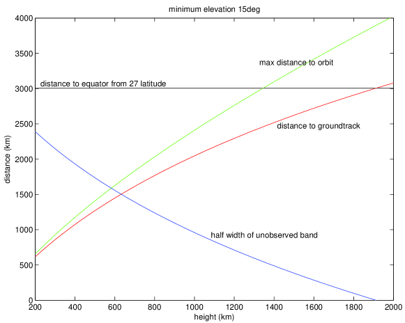
Figure 1: Maximum distance to orbit, to groundtrack and half width of the equatorial unobservable belt

The first constraints to the network architecture are purely geometrical and are due to the horizon. An orbiting object at an altitude $h_{p}$ is visible only up to a given distance from a station, beyond which the object is below a minimum elevation, $15^{\circ}$ being a reasonable value. For an object at $h=1400$ km, the distance to the object is thus limited to about 3100 km, and the distance to the groundtrack of the object to about 2500 km; see Fig. 1, showing these values in km as a function of the object altitude. Moreover, for a station at a latitude of $27^{\circ}$, this Figure also shows the half width of the equatorial band such that, if the groundtrack is in there, the object is not observable. This argument favors the stations located at low latitudes.

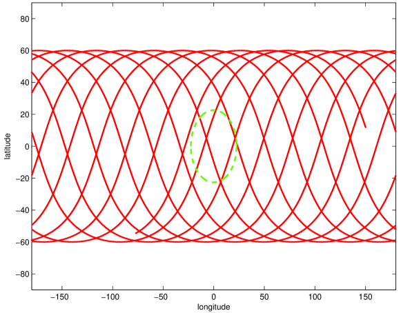
Figure 2: Ground track for $\mathbf{h_{p}}=$ 1400 km, $I=$60^∘

The second consideration is how the object presents itself with a groundtrack passing near a station. Figure 2 shows the groundtrack for a nearly circular orbit with $h_{p}=1400$ km and inclination of 60^∘. The oval contour shows the maximum visibility range, for an equatorial station and an elevation $\geq 15^{\circ}$. Typically a LEO has 4 passes/day above the required altitude as seen from a station at low latitudes. Note that the constraints discussed so far apply equally to a radar sensor.

3.2 Geometry of sunlight

The main difference with radar arises because of the geometry of sunlight. The requirements for an optical station are the following:

1. the ground station is in darkness, e.g., the Sun must be at least 10-12^∘ below the horizon, that is the sky is dark enough to begin operations, typically about 30-60 minutes after sunset and before sunrise (this is strongly dependent on the latitude and the season at the station);

2. the orbiting object is in sunlight;

3. the atmosphere is clear (no dense clouds).

The condition on sunlight is quite restrictive: the low orbiting objects are fully illuminated in all directions only just after sunset and before sunrise. In the Figures 3-5 the bold line represents the Earth shadow boundary at 1400 km above ground. The shadow also depends upon the season, the figures have been drawn for March 20, a date close to an equinox. The Earth shadow region, where the orbiting object is invisible, is represented in gray. The circles represent the iso-elevation regions of the sky above the horizon, which is the outer curve; the center is the local zenith.

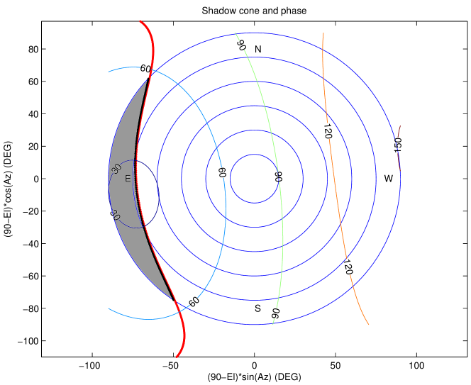
Figure 3: Earth Shadow and iso-phase curves, tropical station at solar time 19 hours

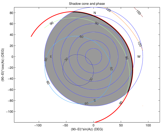
Figure 4: Earth shadow and iso-phase curves, tropical station at solar time 22 hours

The labeled lines (30, 60, 90 and 120) represent the iso-phase curves for objects at 1400 km above ground, that is the directions in the sky where the objects have a specific phase angle. The phase angle is a very critical observing parameter for a debris. The optical magnitude of an object (generally all Solar System moving objects) depends, among other parameters, by the phase angle: the smaller the phase angle the brighter the object. The strength of this effect also depends upon the optical properties of the object surface, such as the albedo. Anyway the effect is large, e.g., at a phase of $90^{\circ}$ the apparent magnitude could increase by $>3$ magnitudes with respect to an object at the same distance but with $0^{\circ}$ phase. Thus an observation scheduling taking into account the need of observing with the lowest possible phase increases very significantly the optical sensor performance.

Figure 5: Earth shadow and iso-phase curves, high latitude station at solar time 22 hours

The Figures show that the regions where the phase angles are smaller are close to the Earth shadow boundary. Very low phases can be achieved only near sunset and sunrise, by looking in a direction roughly opposite to the Sun (see Fig. 3). For LEOs there is a central portion of the night, lasting several hours, in which for a either an equatorial or a tropical station the observations are either impossible or with a very unfavorable phase, e.g., for the station at $27^{\circ}$ North latitude on March 20 from about 22 hours to 2 hours of the next day (see Fig. 4). On the contrary, for a station at an high latitude (both North and South) the dark period around midnight when LEO cannot be observed does not occur, because the Earth shadow moves South (for a North station; see Fig. 5).

3.3 Selection of the observing network

It is clear that, by combining the orbital geometry of passages above the station with the no shadow condition, it is possible to obtain objects which are unobservable from any given low latitude station, at least for a time span until the precession of the orbit (due to Earth’s oblateness, $\sim 5^{\circ}\,\cos I$/day for an altitude of 1400 km and inclination $I$) changes the angle between the orbit plane and the direction to the Sun. On the other hand, high latitude stations cannot observe low inclination objects, and operate for a lower number of hours per year because of shorter hours of darkness in summer and worse weather in winter. A trade off is needed, which suggests to select some intermediate latitude stations, somewhere between 40 and 50^∘ both North and South.

The meteorological constraints can be handled by having multiple opportunities of observations from stations far enough to have low meteorological correlation. This implies that an optimal network needs to include both tropical and high latitude stations, with a good distribution also in longitude. Beside the need for geographic distribution as discussed above, the other elements to be considered in the selection of the network are the following:

• Geopolitics: the land needs to belong to Europe, or to friendly nations. The limitations of the European continent implies that sites in minor European islands around the world are needed as well as observing sites in other countries.

• Logistics: some essentials like electrical power, water supply, telecommunications, airports, harbors, and roads have to be available.

• Meteo: the cloud cover can be extremely high, in some geographic areas, and especially in (local) winter. Other meteorological parameters such as humidity, seeing, wind play an important role. High elevation observing sites over the inversion layer are desirable, but in mid ocean there are not many mountains high enough.

• Orography: an unobstructed view of the needed sky portions, down to 15^∘ of elevation, is necessary. Astronomical observatories are not so demanding, especially in the pole direction.

• Light pollution: an observing site with low light pollution is essential, to lower the sky background, which is the main source of noise.

Table 1: Geographical coordinates of the proposed network of stations

STATION	Latitude [deg]	Longitude [deg]	Height [m]
TEIDE	28∘ 18’ 03.3” N	16∘ 30’ 42.5” W	2390
(Canary Islands, Spain)
HAO	18∘ 08’ 45.0” S	140∘ 52’ 54.0” W	6
(French Polynesia, France)
FALKLAND ISLAND	51∘ 42’ 32.0” S	57∘ 50’ 27.0” W	30
(Great Britain)
NEW NORCIA	31∘ 02’ 54.0” S	116∘ 11’ 31.0” E	244
(Australia)
MALARGUE	35∘ 46’ 24.0” S	69∘ 23’ 59.0” W	1509
(Argentina)
GRAN SASSO	42∘ 29’ 60.0 N	13∘ 33’ 04.0” E	1439
(Italy)
PICO DE VARA	37∘ 47’ 48.0” N	25∘ 13’ 10.0” W	579
(Azores Islands, Portugal)

The optical station network used for our simulations takes into account, as much as possible, the above constraints and is shown on Table. In the selection of the stations we took into account the local meteorological statistics. This was done by accessing meteorological data bases, mostly data obtained from the ISCCP (NASA) project (http://isccp.giss.nasa.gov/index.html). The analysis of these data forced us to give up the possibility of using some geographically convenient locations, which turned out to have a “total cloud amount”, defined as the percentage of cloud coverage of the sky for each day of the year, far too high: e.g., the islands of St. Pierre and Michelon, French territory near Canada, were excluded.

4 Population model

In order to produce a realistic simulation of the whole observation process a suitable population of orbiting objects is required. A subset of the ESA MASTER-2005 population model [24], upgraded with the recent in-orbit collisions (FengYun-1C, IRIDIUM 33 - COSMOS 2251) was provided by ESOC. The MASTER model contains the largest objects taken from the USSTRATCOM Two Line Elements (TLE) plus smaller objects generated with ad hoc source models. The subset available for this work included 31686 entries, representing either single objects or sampled ones, with diameter $d$, 3 cm $<d<$ 31.7 m and crossing the Low Earth Orbit (LEO) region (i.e., with the perigee altitude $h_{p}$ between 200 km and 2000 km).

The population file did not contain any value for the albedo of the objects, a quantity that is needed to derive the magnitude of the object in the sky. A commonly accepted value of the albedo for a generic spacecraft is between 0.1 and 0.2 [1, 11]. We used the conservative assumption of albedo 0.1 for all the objects considered. Then the absolute magnitude $H$ was derived according to the IAU standard for asteroids: $H=33-5\log_{10}(d)$ where $d$ (in m) is provided by the MASTER.

5 Conditions for detection

The possibility to detect an object with an optical sensor depends upon the $S/N$ of the corresponding image. The $S/N$ is a function of the following parameters of the object: $H$, distance, and angular velocity with respect to the image reference frame. The images are taken in a sidereal reference frame, defined by stars. (Only for GEOs there is advantage in taking the images in a reference frame body-fixed to the Earth). The apparent magnitude $h$ can be computed as follows, if the exposure time is such that there is no trailing effect (that is, the image has the same shape as the one of a fixed star):

$$h=H-5\log_{10}(r)+f(\phi,G)$$ (1)

where $r$ is the distance station-object in Astronomical Units, $f$ is the function describing the phase effect, containing the phase angle $\phi$ and a parameter $G$ depending upon the optical properties of the surface. As mentioned above, the correction $f$ is important. The other parameters depend upon the instrument and the atmosphere. The standard equation to compute $S/N$ for a stationary source (a star) is given by the following formula:

$$\left(\frac{S}{N}\right)_{star}=\frac{S}{\sqrt{S+N}}\,.$$

In this formula $N$ includes the contributions from all the sources of noise occurring in the measurement, in particular:

• Read/Out noise: $\sigma^{2}_{r/o}=n_{pix}\,RN^{2}$ (RN = pixel r/o noise);

• Dark current noise: $\sigma^{2}_{Dk}=D\,n_{pix}\,t$ (D = dark current);

• Sky background: $\sigma^{2}_{sky}=R_{sky}\,t$ (R_sky = sky background flux).

The term $S$ under square root accounts for the Poisson statistics: $\sigma^{2}_{Poisson}=S$.

The main problem with optical observations of Earth orbiting objects, especially for LEO, is their large angular velocity in the sidereal frame. Thus, unless the exposure times are very short, severely limiting the maximum magnitude of a detectable object, the image is a trail, spread over a comparatively large number of pixels. The $S/N$ on a single pixel is given by dividing the total signal of the debris by $T$; this effect is called trailing loss. In other words, the signal per pixel is $S/T$, thus on a single pixel:

$$\left(\frac{S}{N}\right)_{pixel}=\frac{{S}/{T}}{\sqrt{{S}/{T}+N}}\ .$$

The values of $S$ as a function of $h$, and of $N$ as a function of the instrument properties and of the atmospheric properties, have been computed on the basis of the telescope design as in [4].

An algorithm to combine the information contained in all the pixels touched by the trail has been proposed by [12]. The principle is to test all the possible trails which could occur in the frame, with a computationally efficient algorithm to decrease the computational complexity. Such an algorithm is capable to detect very faint trails, because the signal along the trail direction is added, while the noise is added in the RMS sense. Thus the $S/N$ for the trail is :

$$\left(\frac{S}{N}\right)_{trail}=\frac{(S/T)T}{\sqrt{T}\sqrt{S/T+N}}=\frac{S}{\sqrt{S+NT}}\ .$$ (2)

Then the $S/N$ of the trail is much larger than the single pixel one by a factor close to $\sqrt{T}$ for low $S$. According to the tests reported in [12], it is necessary to keep some margin to avoid false detections of trails, thus we use as criterion ${S}/{N}_{trail}\geq 6$, while for a stationary object lower values, such as 3, could be used. E.g., for a trail $T=200$ pixels long, the advantage is by a factor $\sqrt{200}/2\sim 7$, equivalent to more than 2 magnitudes. Fig. 6 shows the $S/N$, as a function of the $h$, for different observing conditions, resulting in different values of the trailing loss parameter $T$. From the top: for a fixed star; for angular velocity $300$ arcsec/s; for $1000$ arcsec/s; on each individual pixel (for $300$ arcsec/s).

Figure 6: $h$ vs. $S/N$, for different trailing loss: from the top, $T$=1, 200, 600

The problem is that it is not easy to determine the beginning and the end of the trail with high accuracy when the trail is too faint. For faint trails, the astrometric error is determined by the error in finding the ends, thus is given by:

$$Z\left(\frac{S}{N}\right)_{pixel}\leq\sqrt{Z}\Longrightarrow Z=\frac{TS+T^{2}N}{S^{2}}=\left(\frac{1}{(S/N)_{pixel}}\right)^{2}\ .$$ (3)

In practice there are two regimes for the astrometric error:

• when the signal is strong, the astrometric error is dominated by the astrometry method, that is by the systematics in the astrometric catalogs;

• when the signal is weak, the astrometric error is determined by (3), see Fig. 6.

Fig. 6 shows also the astrometric error, in arcsec, for angular velocity $300$ arcsec/s (broken line).

6 Correlation and orbit determination

Given two or more observations sets, the main problem is to identify which data belong to the same object (correlation problem). Thus the orbit determination problem needs to be solved in two stages: first different sets of observations need to be correlated, then an orbit can be determined.

6.1 Observations and attributables

When a LEO is observed optically, even a comparatively short exposure results in a trail. The detection of the trail, with the method discussed in Sec. 5, is followed by the astrometric reduction of the two ends of the trail. When the trail is too short to show measurable curvature [16], the information contained in these two data points can be summarized in an attributable:

$${\cal A}=(\alpha,\delta,\dot{\alpha},\dot{\delta})\in[0,2\pi)\times(\pi/2,\pi/2)\times\mathbb{R}^{2}\,,$$

representing the angular position and velocity of the body at a time $t$. Usually $\alpha$ is the right ascension and $\delta$ the declination with respect to an equatorial reference system (e.g., J2000).

To compute a 6 parameters orbit, we need 2 further quantities. The values of range $\rho$ and range rate $\dot{\rho}$ are not measured. These two quantities, together with ${\cal A}$, allow us to compute the the Cartesian position and velocity $(\mathbf{r},\dot{\mathbf{r}})$ at time $\bar{t}=t-\rho/c$:

$$\mathbf{r}=\mathbf{q}+\rho\hat{\bm{\rho}}\ \ ,\ \ \dot{\mathbf{r}}=\dot{\mathbf{q}}+\dot{\rho}\hat{\bm{\rho}}+\rho\frac{d\hat{\bm{\rho}}}{dt}\ \ \ ,\ \ \ \frac{d\hat{\bm{\rho}}}{dt}=\dot{\alpha}\hat{\bm{\rho}}_{\alpha}+\dot{\delta}\hat{\bm{\rho}}_{\delta}\ ,$$ (4)

$$\hat{\bm{\rho}}=(\cos\alpha\cos\delta,\sin\alpha\cos\delta,\sin\delta)\,,\ \ \ \hat{\bm{\rho}}_{\alpha}=\partial\hat{\bm{\rho}}/\partial\alpha\,,\ \ \ \hat{\bm{\rho}}_{\delta}=\partial\hat{\bm{\rho}}/\partial\alpha\,.$$

In the above formulae the observer position $\mathbf{q}$ and velocity $\dot{\mathbf{q}}$ are known functions of time.

6.2 Keplerian integrals method

In our simulations we used the Keplerian integrals method to produce preliminary orbits from two attributables ${\cal A}_{1}$, ${\cal A}_{2}$ of the same object at two epoch times, $t_{1}$ and $t_{2}$. This is used as the first, the most difficult, step of the correlation procedure. The algorithm for the asteroid case is introduced in [9], while in [6] it is adapted to space debris. The method has already been successfully applied to the orbit determination of GEOs in [19]. We recall here the basic steps.

Using (4), the 2-body energy ${\cal E}$ and the angular momentum $\mathbf{c}$ can be expressed as function of ${\cal A}$, $\rho$ and $\dot{\rho}$. If the orbit between $t_{1}$ and $t_{2}$ is well approximated by a Keplerian one, we have:

$$\begin{cases}{\cal E}({\cal A}_{1},\rho_{1},\dot{\rho}_{1})-{\cal E}({\cal A}_{2},\rho_{2},\dot{\rho}_{2})=0\\ \mathbf{c}({\cal A}_{1},\rho_{1},\dot{\rho}_{1})-\mathbf{c}({\cal A}_{2},\rho_{2},\dot{\rho}_{2})=0\end{cases}\ \ \ \rho_{1}>0\ ,\ \rho_{2}>0\,.$$ (5)

From a solution of the above system we obtain 2 sets of orbital elements at times $\bar{t}_{1}$ and $\bar{t}_{2}$:

$$(a_{j},e_{j},I_{j},\Omega_{j},\omega_{j},\ell_{j})\ ,\ j=1,2\ .$$

where $a$ is the semimajor axis, $e$ the eccentricity, $\Omega$ the longitude of node, $\omega$ the argument of perigee, and $\ell$ the mean anomaly. The first four Keplerian elements $(a_{j},e_{j},I_{j},\Omega_{j})$ are functions of the 2-body energy and angular momentum vectors ${\cal E}_{j}$, $\mathbf{c}_{j}$, and are the same for $j=1,2$. In addition, there are compatibility conditions to be satisfied if the two attributables belong to the same object:

$$\omega_{1}=\omega_{2}\ ,\ \ell_{1}=\ell_{2}+n(\bar{t}_{1}-\bar{t}_{2})\ ,$$ (6)

where $n=n(a)$ is the mean motion. The algorithm also provides a covariance matrix for the computed orbit and a $\chi$ value to measure the discrepancy in the compatibility conditions. If such $\chi$ is smaller than some maximum value $\chi_{max}$ the orbit is accepted.

6.3 Precession model

To deal with LEOs it is necessary to generalize the method, including the effect due to the Earth oblateness. The secular equations for Delaunay’s variables $\ell$, $\omega$, $\Omega$, $L=\sqrt{\mu a}$, $G=L\sqrt{1-e^{2}}$ and $Z=G\cos I$ are (e.g., [21][Sec. 11.4]):

$$\begin{cases}\displaystyle\bar{\dot{\ell}}=n-\frac{3}{4}n\left(\frac{R_{\oplus}}{a}\right)^{2}\frac{J_{2}(1-3\cos^{2}I)}{(1-e^{2})^{3/2}}\\ \stackrel{{\scriptstyle}}{{\displaystyle\bar{\dot{\omega}}=\frac{3}{4}n\left(\frac{R_{\oplus}}{a}\right)^{2}\frac{J_{2}(4-5\sin^{2}I)}{(1-e^{2})^{2}}}}\\ \stackrel{{\scriptstyle}}{{\displaystyle\bar{\dot{\Omega}}=-\frac{3}{2}n\left(\frac{R_{\oplus}}{a}\right)^{2}\frac{J_{2}\cos I}{(1-e^{2})^{2}}}}\\ \stackrel{{\scriptstyle}}{{\bar{\dot{L}}=\bar{\dot{G}}=\bar{\dot{Z}}=0}}\end{cases}\ ,$$ (7)

where $J_{2}$ is the coefficient of the second zonal spherical harmonic of the Earth gravity field and $R_{\oplus}$ is the Earth radius. In this case we cannot use the conservation of angular momentum, since it precedes up to $5^{\circ}\cos I$ /day. Thus we consider the parametric problem obtained by imposing $\dot{\Omega}=K$, with $K$ constant:

$$\begin{cases}{\cal E}_{1}-{\cal E}_{2}=0\\ R\,\mathbf{c}_{1}-R^{T}\,\mathbf{c}_{2}=0\end{cases}$$ (8)

where $R$ is the rotation by $\Delta\Omega/2=K(\bar{t}_{2}-\bar{t}_{1})/2$ around $\hat{\mathbf{z}}$. Thus for a fixed value of $K$ the problem has the same algebraic structure of the unperturbed one. The compatibility conditions contain the perigee precession and the secular perturbation in mean anomaly, related to the one of the node by

$$\omega_{1}=\omega_{2}+KC_{\omega}\,(\bar{t}_{1}-\bar{t}_{2})\,,\ \ \ell_{1}=\ell_{2}+(n+KC_{\ell})(\bar{t}_{1}-\bar{t}_{2})\,,$$

where $C_{\omega},C_{\ell}$ can be deduced from (7). Thus we can compute the $\chi(K)$.

We set up a fixed point iterative procedure, defined as follows:

1. given the orbital elements $E_{i}$ at step $i$ we compute the corresponding value of $K$ by (7);

2. for the computed value of $K$ we solve the corresponding system (8);

3. we select the solution with lowest $\chi$ and compute the corresponding orbital elements $E_{i+1}$;

4. we start again from 1, until convergence.

To find a starting guess we select a value $K_{0}$ either using the circular orbits corresponding to each of the two attributables (see [7]) or by assuming $K_{0}=0$. Among the obtained solutions, we cannot know which one could lead to convergence. Since the value of $K_{0}$ is quite arbitrary, it is not safe to select only those with a low value of $\chi$. Thus we use all the solutions as possible starting guess for the iterative procedure.

6.4 Correlation confirmation

The orbits obtained using the methods described in the previous sections are just preliminary orbits, solution of a 2-body approximation, or possibly of a $J_{2}$-only problem. They have to be replaced by least squares orbits, with a dynamical model including all the relevant perturbations.

Even after confirmation by least squares fit, some correlations can be false, that is the two attributables might belong to different objects. This is confirmed by the tests with real data reported in [19] and [9]. Thus every linkage of two attributables needs to be confirmed by correlating further attributables. The process of looking for a third attributable which can also be correlated to the other two is called attribution [13, 14]. From the available 2-attributable orbit with covariance we predict the attributable ${\cal A}_{P}$ at the time $t_{3}$ of a third attributable ${\cal A}_{3}$, and test the compatibility with ${\cal A}_{3}$. For the successful attributions we proceed to the differential corrections.

The procedure is recursive, that is we can use the 3-attributable orbit to search for attribution of a fourth attributable, and so on. This generates a very large number of many-attributable orbits, but there are many duplications, corresponding to adding them in a different order. Thus a normalization step is needed to remove duplicates (e.g., $A=B=C$ and $A=C=B$) and inferior correlations (e.g., $A=B=C$ is superior to both $A=B$ and to $C=D$, thus both are removed). This procedure, called correlation management, is important to reduce the risk of false correlation, because they are eliminated by superior and discordant true correlations [15]. As an alternative, we may try to merge two discordant correlations (with some attributables in common), by computing a common orbit. For a description of the sequence of steps in this procedure see [16].

6.5 Updating well constrained orbits

When an orbit is very well constrained and the number of involved trails is high enough, the possibility for the corresponding correlation to be false can be ruled out. In this case the corresponding object is cataloged and numbered (that is, the object is given a unique identifier). There are no fixed rules for space debris to establish whether an object can be numbered. Our (safe but arbitrary) criterion was the following: if the correlation involves more than 10 trails the object is numbered. This criterion makes sense, since 10 trails, with an observing strategy giving only one exposure per pass, corresponds to many revolutions of the object.

When an object is numbered, or anyway when the number of trails is significant, it is possible to use the orbit with its covariance as a basis for attribution of other trails to the same object. This procedure should be done before attempting to find previously unknown objects in the data, to reduce the data set to which the most computationally complex procedure is applied. This is especially necessary because the brightest objects are observed much more often than the others. If the procedure of attribution of trails to known objects is successful, after few weeks from the beginning of the catalog build-up the leftover trails to be correlated are comparatively few.

Note that the procedure outlined in this section essentially amounts to a simulation not just of the performance of the sensors network, but also of the operations of an orbit determination data center. The performance of this element of a space awareness system is by no means less important than the performance of the observing hardware.

7 Results of the Catalog build-up simulation

The first simulation was the one of the catalog build-up. Namely, we assumed to start with no information on the satellite/debris population in the region of interest (high LEO) and attempted to build up an orbit catalog, to be compared with the MASTER one. For this purpose we conducted a large scale simulation, with two different population samples, dubbed Population 1 and 2.

7.1 Population samples

Population 1 was made up of 912 objects, randomly selected among those with $8<d<27$ cm, and $1300\leq h_{p}<2000$ km. Population 2 included 1104 objects, with $5<d<25$ cm, and $1000\leq h_{p}<1300$ km. Objects larger than 27 cm and 25 cm respectively were not included in the simulation, since the amount of observational data allows us to attain a complete catalog in a comparatively short time span. This is confirmed not only by some preliminary tests but also by the analysis of this simulation, which shows that all the objects larger than 20 cm are cataloged within 1 month.

These choices were driven by the hypothetical performances of an enhanced radar sensor, to be used along with the optical ones in the ESA-SSA program. Figure 7 shows two rectangles on the perigee altitude-diameter plane, which enclose the regions corresponding to the selected population samples. For the considered values of the perigee altitude, we have drawn two curves, representing the observing capabilities of a baseline radar and of an enhanced radar. The corresponding assumptions on the radar systems are rather arbitrary, thus these performance curves have to be considered just as a comparison benchmark: indeed, the purpose of the investigation was to determine the requirement for a future radar system, and to see how much this could change by assuming the cooperation of a network of optical sensors. These curves give the minimum diameter $d_{min}$ of observable objects as function of $h_{p}$, according to the following law:

$$d_{min}=\frac{h_{p}^{2}}{h_{ref}^{2}}d_{ref}\,,$$ (9)

where $h_{ref}$ and $d_{ref}$ are reference values for the perigee altitude and the diameter. The equation (9) is a simple consequence of the inverse fourth power dependence of radar $S/N$ from distance. We set $h_{ref}=2000$ km and $d_{\rm ref}=32$ cm for the baseline radar. For the enhanced radar we took $h_{ref}=2000$ km and $d_{ref}=20$ cm. The two rectangles containing the populations used in the simulation cover a region including the performance curve of the enhanced radar.

To analyze the results, we split the population in three orbital classes:

• LEO: LEO resident objects, with semimajor axis $a\leq R_{\oplus}+$ 2000 km;

• PLEO: “partial LEO”, with perigee inside but apogee beyond the LEO region: $h_{p}<2000$ km, $a>R_{\oplus}+2000$ km, and limited eccentricity, so that $a<25000$ km;

• HLEO: LEO transit objects, with $h_{p}<2000$ km and large eccentricity, so that $a\geq 25000$ km. This class includes in particular GTO and Molniya objects.

The HLEO objects spend only a small fraction of their orbital period below $2000$ km of altitude, and have a large velocity when at perigee, thus an angular velocity with respect to the observing station larger than the resident LEO. Thus they are much more difficult to be observed by the network selected for resident LEO. They could be the target of a survey with a completely different observing strategy. E.g., the GTO orbits can be observed with longer exposures and non-sidereal tracking while near apogee [22]. Thus the results in our simulations about HLEO are not very significant: these objects should be considered in the context of a simulation with an observing strategy adapted to higher orbits, such as MEO.

In the MASTER population model, smaller objects typically are sampled, i.e. a single object represents many fragments. Simple de-sampling (e.g., by assigning different mean anomalies to each fragment, keeping all the other orbital elements the same) could affect our simulations by generating false correlations. Therefore the sampled fragments were treated as single objects in the simulation process. A sampling factor was associated to each object to represent the number of fragments within the same orbit in the final analysis of the results.

7.2 Results

Figure 7 shows the results of both population samples in the perigee altitude-diameter plane after 2 months of survey observations. The rectangles enclose the regions of the plane corresponding to the selected population samples. The parabolic curves represent two possible radar performances in the case of a baseline radar (dashed line) and of an enhanced one (solid line). The top figure shows the results for resident LEOs, while the bottom one is for transit objects (PLEOs and HLEOs). Points indicate successful orbit determination ($\geq$ 3 trails involved), while circles correspond to failure. The reasons for the occurrence of this last possibility are essentially three:

1. lack of observations;

2. the observations were very few and too distant in time, so that correlation was not possible;

3. the observations had low accuracy, so that even when the correlation of two trails was successful, the orbit accuracy was not enough for the attribution of further trails.

For LEOs, there are many failures only in the low part of the region corresponding to Population 2. This means that this possibility can happen only for some very small objects, with diameter $<8$ cm.

Figure 7: Results of catalog build-up after 2 months

Tables 2 and 3 detail the results for each population sample. The factor associated to the sampled objects is not taken into account. This means that a group of fragments with the same orbit is treated as a single object. In the tables are reported in this order the total number of objects in the sample, the number of cataloged objects, the number of objects observed but not cataloged, and the number of never observed objects. The row in parenthesis contains the number of objects, among those with some observations but without orbit, for which a total of only 1-2 trails were available in 2 months of survey.

Table 2: Results of catalog build-up after 2 months, Population 1

POP 1	Total	LEO	PLEO	HLEO
No. Objects	912	796	97	19
Orbits Computed	894	793	95	6
Obj. without orbit	10	3	2	5
(with 1-2 Tr.)	(3)	(0)	(0)	(3)
Obj. not observed	8	0	0	8

Table 3: Results of catalog build-up after 2 months, Population 2

POP 2	Total	LEO	PLEO	HLEO
No. Objects	1104	1014	62	28
Orbits Computed	965	942	21	2
Obj. without orbit	92	67	16	9
(with 1-2 Tr.)	(13)	(9)	(2)	(2)
Obj. not observed	47	5	25	17

To analyze the results, we measured the efficiency of the catalog build-up, defined as the ratio between the number of reliable orbits computed (with at least 3 trails) and the total number of sampled objects. We measured also the efficiency only for those objects lying in the region of the perigee altitude-diameter plane above the curve of the enhanced radar. These efficiencies were computed accounting for the number of clones for the sampled objects (sampling factor), to count both the successes and the failures of correlation. The detailed results are shown in Tables 4 and 5.

Table 4: Efficiency of catalog build-up after 2 months, Population 1

POP 1	Total	LEO	PLEO	HLEO
Eff. Catalog	98.1%	99.6%	97.9%	31.6%
Eff. above Radar	98.6%	99.8%	97.2%	71.4%

Table 5: Efficiency of catalog build-up after 2 months, Population 2

POP 2	Total	LEO	PLEO	HLEO
Eff. Catalog	82.8%	86.6%	37.5%	7.1%
Eff. above Radar	93.7%	98.9%	97.2%	25.0%

The results for Population 1 were overwhelming. For $h_{p}>1300$ km, we computed the orbits of almost all the objects above 8 cm ($98.1\%$) and of $99.6\%$ of resident LEOs. If we consider only the objects above the curve of enhanced radar performance in Fig. 7, then the total efficiency is $98.6\%$, while for resident LEOs it is $99.8\%$. A few objects in highly eccentric transit orbits (e.g., GTO) were lost, but they should be observed with a different strategy, as outlined previously.

For Population 2 the total efficiency is $82.8\%$, while considering only resident LEOs it is $86.6\%$; if we take into account only the region above the curve of the enhanced radar the corresponding percentages are $93.7\%$ and $98.9\%$. Moreover, the outcome of the two simulations suggests that the problem is not the altitude but the diameter: indeed, even for Population 2, among the objects larger than 8 cm, $95.8\%$ had a reliable orbit, and for resident LEOs the percentage was $99.0\%$. Smaller debris require a larger telescope, whatever the height.

To get the big picture of the results, we should take into account also the biggest objects of the MASTER population. Moreover, the results of Population 1 have to be weighted twice, since we randomly selected only half of the objects. By assuming that all the biggest objects were cataloged after 2 months of survey, we get an overall efficiency 97.9% for the objects above the enhanced radar curve. By considering only LEOs the efficiency is 99.0%. Figure 7 shows that most of the difficulties in the catalog build-up concern the region of orbital perigee altitude less than $1100$ km. If we discard this region, the total efficiency reaches 98.9%, and for LEOs 99.8%.

8 Orbit improvement phase

Tasking observations are possible if, by moving the telescope at non-sidereal rate, the object remains in the telescope field of view. This is achieved if the angular error in prediction is small enough. Moreover, it is desirable to see the object with most signal concentrated on a single pixel, thus obtaining a higher signal with respect to the survey mode.

8.1 Feasibility of tasking observations

We considered the numbered objects obtained after 1 month of catalog build-up and we propagated the orbits for 1 week after the last observation. Then the angular error in prediction and the relative error in angular velocity were computed, by means of the covariance matrices.

Denoting by $\Gamma_{P}$ and $\Gamma_{V}$ the marginal covariance matrices for position and velocity respectively, and by $\lambda_{P},\lambda_{V}$ their maximum eigenvalues, we used the following upper bounds for the angular error and the relative error in velocity:

$$\Delta(\alpha,\delta)\leq\frac{\sqrt{\lambda_{P}}}{h_{p}}\,,\quad\frac{|\Delta{\bf v}|}{|{\bf v}|}\leq\frac{\sqrt{\lambda_{V}}}{|{\bf v}|}\ .$$

These approximations are justified for LEOs by the fact that they move on almost circular orbits, so that the radial component of the velocity is small. On the other hand high eccentricity transit objects are observed near the perigee.

Taking into account that the angular velocity of the objects in our sample was less than 2000 arcsec/s, to see the object in a single pixel during tasking, the relative error in angular velocity had to be less than $7.5\times 10^{-4}$. This was achieved for all the numbered objects. Moreover the angular error in position was always less than 95 arcsec. Then the possibility of follow up was confirmed and we were allowed to take $T=1$ (no trailing loss) in the $S/N$ formula, with a gain in $S/N$ for faint objects by a factor at least 14.

Besides assuming $T=1$, we supposed the scheduler to be capable of selecting 1/6 of the observation period, corresponding to the best phase angle, thus gaining more than 1 magnitude with respect to survey observations. The combination of these two effects increases the number of observations, because a trail with a very low $S/N$ in survey mode becomes detectable in tasking mode as a point source; in addition, in many cases the astrometric accuracy is significantly improved.

To perform the follow up simulation, we chose the same two populations used for the survey step, but we excluded HLEOs, since the observation strategy was not suitable for this kind of objects, as confirmed by the results of the catalog build-up. At the starting time of the simulation, the sampled objects were assumed to be cataloged with sufficiently well determined orbits. Thus, we assumed that the switch to tasking mode occurred for all the cataloged orbits at the same time. In reality, the decision to include an object in the tasking mode scheduling should be performed on an individual basis. The same procedure of the survey simulations was adopted, meaning that the previously computed catalog was not used and the orbit determination was performed again from scratch. The difference was in the kind and the amount of data, as follow up observations were more numerous and accurate than the survey ones.

8.2 Accuracy envelope norm

The orbit improvement goal was defined by choosing an accuracy envelope to which compare the accuracy of the computed orbits. First we fixed the object-centered reference frame $\{\mathbf{u},\mathbf{v},\mathbf{w}\}$, where $\mathbf{u}$ is the direction from the Earth center to the object center, $\mathbf{w}$ is the direction of the angular momentum vector and $\mathbf{v}=\mathbf{w}\times\mathbf{u}$. Then the accuracy ellipsoid in position for resident LEOs was defined by the quantities $4,30,20$ m along the directions $\mathbf{u},\mathbf{v},\mathbf{w}$ respectively, for PLEOs by $10,60,200$ m. The accuracy ellipsoid in velocity was $20,4,20$ mm/s both for resident LEOs and PLEOs. These ellipsoids were derived from collision avoidance requirements.

To see if the improved orbits were inside the envelope, we had to verify that the confidence ellipsoids, representing the uncertainty of the orbits in position and velocity, were fully contained in the ellipsoids defined by the accuracy envelope.

Let $\mathbf{C}_{req}$ be the marginal normal matrix associated to the accuracy envelope for position (for LEOs, $\mathbf{C}_{req}=diag[1/4^{2},1/30^{2},1/20^{2}]$ in the OCRF), and let $\mathbf{C}_{conf}$ be the marginal normal matrix of the orbit. Then the two ellipsoids relative to position are defined respectively by the equations

$$\mathbf{x}^{T}\mathbf{C}_{req}\mathbf{x}=1\,,\quad\mathbf{x}^{T}\mathbf{C}_{conf}\mathbf{x}=1\,.$$

To satisfy the envelope, the maximum of the function $\mathbf{x}^{T}\mathbf{C}_{req}\mathbf{x}$, as $\mathbf{x}$ varies in the confidence ellipsoid of the orbit, must be less than 1. By Lagrange multiplier theorem a necessary and sufficient condition for this is that $\lambda\leq 1$, for any $\lambda$ for which $\det(\mathbf{C}_{req}-\lambda\mathbf{C}_{conf})=0$.

Let $\mathbf{\Gamma}_{req}=\mathbf{C}_{req}^{-1}$ and $\mathbf{\Gamma}_{conf}=\mathbf{C}_{\rm conf}^{-1}$ denote the marginal covariance matrices and let $\mathbf{P}_{req}$ a matrix such that $\mathbf{C}_{\rm req}=\mathbf{P}_{req}^{T}\mathbf{P}_{req}$ (it exists, because $\mathbf{C}_{req}$ is symmetric and non-negative). Then the values of $\lambda$ such that $\det(\mathbf{C}_{req}-\lambda\mathbf{C}_{conf})=0$ are the eigenvalues of the matrix $\mathbf{P}_{req}\mathbf{\Gamma}_{\rm conf}\mathbf{P}_{req}^{T}$. Thus we defined the accuracy envelope norm in position as the square root of the maximum eigenvalue of the matrix $\mathbf{P}_{req}\mathbf{\Gamma}_{conf}\mathbf{P}_{req}^{T}$. For the velocity we used a completely analogous definition.

8.3 Results

The simulation covered three weeks of tasking. All the numbered orbits were propagated for 1 week after the last observation and compared to the accuracy envelope. The comparison was performed through the accuracy envelope norm previously defined, which is $\leq 1$ whenever the uncertainty is smaller than the envelope.

Tables 6 and 7 summarize the results for LEOs after the first and the third week respectively. The values reported are: percentage of objects with accuracy envelope norm $\leq 1$ in both position and velocity, maximum norms achieved, maximum angular error in position, percentage of objects with angular error $\leq 1.5$ arcsec (the pixel size). For PLEOs the results are not statistically representative, because in both simulations they were less then 100 objects.

The conclusion of the orbit improvement simulation is that just one week of data is not enough, even with the higher observation frequency and accuracy of the tasking phase, while 3 weeks are more than enough.

Table 6: Results for LEOs after 1 week of tasking

LEO	norms	max norm	max norm	max ang.	ang. err.
1 WEEK	$\leq 1$	position	velocity	err. (arcsec)	$\leq 1.5$ arcsec
POP. 1	76.8%	5.69	5.19	12.96	79.2%
POP. 2	68.6%	6.18	6.5	24.12	63.1%

Table 7: Accuracy of the results for LEOs after 3 weeks of tasking

LEO	norms	max norm	max norm	max ang.	ang. err.
3 WEEKS	$\leq 1$	position	velocity	err. (arcsec)	$\leq 1.5$ arcsec
POP. 1	99.5%	1.25	1.09	2.88	98.2%
POP. 2	99.9%	1.03	0.97	2.88	94.3%

Figure 8 shows the results after 3 weeks. The top figure is for resident LEOs while the bottom one is for PLEOs. Points indicate that both the accuracy norms in position and velocity are $\leq 1$, while circles mean that one of the above norms is $>1$. It turns out that we succeeded for most of LEOs, while there were a few problems for low altitude PLEOs.

Figure 8: Results of both simulations after 3 weeks of tasking

Finally, it must be stressed that the relative error in velocity prediction was always less than $10^{-4}$, which means that with tasking observations there is no trailing loss.

9 Fragmentation detection

A particularly demanding situation for a surveillance network occurs whenever a fragmentation happens in Earth orbit. The resulting cloud of fragments can pose significant immediate or short term risks for other space assets in the same orbital region [20]. Therefore two ad hoc simulations were performed to verify the capability of our proposed optical network to detect and characterize a fragmentation event in high LEO. In general terms, the detection of fragmentation implies to detect a significant number of fragments. Another possibility is to detect the change in the orbital elements of the target object due to the energy of the event. Note that, in the case of an active satellite, if no other information is available, it could be difficult to discriminate between a change due to a maneuver and a collision.

We simulated the fragmentation of a satellite due to both an explosion and a catastrophic collision. To produce the cloud of fragments we used, for both cases, the ISTI implementation of the NASA-JSC model [10].

Given a mass $M_{T}$ of the target object, a cloud of fragments was generated with the proper size distribution given by the NASA model. According to the model, each fragment was characterized by the following elements: size $d$, mass, area, $\Delta v$. From the whole cloud of fragments, we selected those objects with $d>10$ cm and $\Delta v<100$ m/s, that is we concentrated on the core of the cloud. Given the Cartesian coordinates of the parent body, the isotropic $\Delta v$ relative to each fragment was added to these coordinates, thus obtaining the state vector of each fragment. From the Cartesian coordinates, the orbital elements of each fragment were then computed. The orbital elements of the fragments were then propagated for 21 days and the simulated observations were computed. The simulations assumed observations in survey mode, with trailing loss.

First we simulated the explosion of a satellite with mass $M_{T}=1000$ kg. The satellite was supposed to be on a circular orbit at 1400 km of altitude, with an inclination of $74^{\circ}$. The model produced a cloud of 230 fragments larger than 10 cm. Out of them, 175 fragments had $\Delta v<100$ m/s (and 8 fragments had $\Delta v<10$ m/s). The detection of the fragments by the whole network of 7 ground stations was simulated. During the first day after the explosion it was not possible to detect any debris, while, in the second and in the third day, about half of the debris were detected (26.3 % in the second day, 57.7 % in the third day and already 98.9 % in the fourth day). This situation depends on the fact that in the first day the fragments cloud had still a non-homogeneous distribution around the Earth. The debris created by the explosion formed a cloud concentrated around the explosion point. Therefore, in the first hours after the event, the detection of the concentrated cloud was similar to the detection of a single object. If the cloud was not passing in the right moment of the night above a station with favorable meteorological conditions, its detection was not possible. On the contrary, a few days after the explosion, all the debris were detected because they had a homogeneous distribution in a torus around the parent body orbit. It is therefore important to remind that the debris detection after a fragmentation depends on the ground station meteorological data. In particular, in the first day only 2 ground stations were able to observe debris, but the debris cloud was not passing over these stations.

In the second simulation, the collision of a debris with mass 10 kg, against a satellite with mass $M_{T}=1000$ kg, with an impact velocity of $v=9$ km/s, was simulated. In the NASA model, a collision is considered catastrophic whenever the ratio between the kinetic energy of the projectile and the mass of the target exceeds $40\,000$ J/kg. This condition is largely satisfied by our event, so we are considering a catastrophic collision. The target satellite was supposed to be on the same orbit as in the explosion case. The model produced a cloud of 998 fragments larger than 10 cm. Out of them, 393 fragments had $\Delta v<100$ m/s (and 7 fragments had $\Delta v<10$ m/s). The evolution of the cloud of fragments was similar to the one discussed in the explosion case.

The detection statistics was similar to the one for the explosion case (33.6 % of detected objects in the second day, 57.7 in the third day, 66.4 in the fourth day and 99.7 % in the fifth day) and the same considerations about the meteorological conditions apply here. In the first day after the collision only 2 ground stations were able to observe some debris.

After simulating the observations performed by the ground network, we started the correlation and orbit determination process, to check how soon after the event it is possible to have robust information on the fragmentation. Clearly, if 2 days were enough to observe a quite high percentage of fragments, they were not enough to compute reliable orbits for the observed fragments. There were too few observations and in fact no orbits were available after only two days for both the simulations. After 4 days the situation improved and 90 orbits for the collision fragments and 46 orbits for the explosion fragments were computed, if we considered as acceptable correlations of at least 3 trails and discarded the ones between only 2 trails. By comparison with the ground truth (i.e., with the original fragments generated in the simulations) we found that some of the correlations were false, that is they put together observations of different objects. Anyway, all the false correlations had only 3 trails and this was true for both the simulations in the entire period examined. Note that, in the case of the fragments clouds, it is quite natural to have false correlations even among 3 trails, because all the fragments have very similar orbits. To exclude false correlations, in this peculiar case, we considered only orbits fitting $\geq$ 4 trails.

In our analysis we considered as reliable the orbits which fit at least 5 trails and as numbered the orbits with at least 10 trails. We found that, after only 2 weeks, all the objects were numbered both in the explosion and in the collision case. Table 8 gives the summary of the orbit determination process, by showing the number of orbits computed with at least 5 and 10 trails, for both clouds in the two weeks following the fragmentation events.

The graphical tool commonly used to characterize an in-orbit fragmentation is the Gabbard diagram, plotting the apogee/perigee height of the fragments as a function of their orbital period. Figure 9 shows the Gabbard diagram (circles for apogee, crosses for perigee) for the collision case, 6 days after the event. The X-shape, a typical signature of a fragmentation, is already visible.

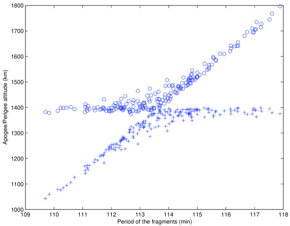
Figure 9: Gabbard diagram of the collision fragments cataloged within 6 days after the event

Table 8: Computation of the orbits of fragments for both explosion and collision

	Explosion		Collision
Days after	Orbits	Orbits	Orbits	Orbits
fragmentation event	$\geq 5$ trail	$\geq 10$ trails	$\geq 5$ trail	$\geq 10$ trails
2	0	0	0	0
4	26	0	63	0
6	99	62	192	141
8	139	124	307	287
10	154	149	333	329
12	169	169	366	366
14	175	175	392	392
16	175	175	393	393

In conclusion, our study suggests that the simulated network of telescopes can detect and catalog the fragments generated by a catastrophic event in high LEO after just a few days from the event. Some caveats and conclusions can be stated. First, the detection of a stream of fragments, with low ejection velocity, within 24 hours is like detecting a single object, because the fragments are not spread along the entire orbit. For this reason it might not be possible to detect a large fraction of the fragments in 1 day, if bad meteorological conditions are present on critical stations. Then, the Gabbard diagram, built with the output of the orbit determination simulation after 6 days, shows that the orbital information is more than enough to assess the fragmentation event (parent body, energy, etc.).

10 Conclusions

The results of the catalog build-up simulation show that more than 98% of the LEO objects with perigee height above 1100 km and diameter greater than 8 cm can be cataloged in 2 months. As Fig.7 shows, a central area around 1100 km of orbital perigee altitude has been identified where radar sensors and the optical network should operate in a cooperative way. All the numbered orbits are accurate enough to allow follow up observations with no trailing loss, and the orbit accuracy from the improved orbits is compliant with the accuracy we have used, which corresponds to collision avoidance requirements. Finally the simulated network of telescopes is able to detect and catalog the fragments generated by a catastrophic event just a few days after the event.

The significance of our results for the design of a Space Situational Awareness system is in the possibility to use optical sensors to catalog and follow up space debris on orbits significantly lower than those previously considered suitable. Of course this is true only provided a list of technological assumptions, both in hardware and in software, spelled out in Section 2, are satisfied. If these technologies are available, then it is possible to trade off between an upgraded system of optical sensors and a radar system with higher energy density.

Aknowledgments

We wish to thank CGS for providing us with the expected sensor performances and realistic simulated observations, taking into account the characteristics of the Fly-Eye telescope, the meteorological model to account for cloud cover, and the statistical model for the signal to noise ratio. This work was performed under ESA/ESOC contract 22750/09/D/HK SARA-Part I Feasibility study of an innovative system for debris surveillance in LEO regime, with CGS as prime contractor.

References

- [1] Africano, J. L., Stansbery, E. G., Kervin, P. W.,“ The optical orbital debris measurement program at NASA and AMOS”, Advances in Space Research, Vol. 34, No. 5, pp. 892–900, 2004.
- [2] Bowell E., Hapke, B., Domingue, D., Lumme, K., Peltionemi, J., Harriw, A. W., “Application of photometric models to asteroids”, Asteroids II, Proceedings of the Conference, University of Arizona Press, Tucson, 1989, pp. 524–556.
- [3] Chesley, S. R., Baer, J., Monet, D. G., “Treatment of star catalog biases in asteroid astrometric observations”, Icarus, Volume 210, No. 1, pp. 158–181, 2010.
- [4] Cibin, L., Besso, P. M., Chiarini, M., Milani Comparetti, A., Ragazzoni, A., “Debris telescopes catch objects in LEO zone”. IAC-10-A6.5.10 (2010).
- [5] Escobal, P. R., Methods of orbit determination. New York: Wiley, 1965.
- [6] Farnocchia, D., Tommei, G., Milani, A., Rossi, A., “Innovative methods of correlation and orbit determination for space debris”, Celestial Mechanics and Dynamical Astronomy, Vol. 107, No. 1–2, pp. 169–185, 2010.
- [7] Fujimoto K., Maruskin J. D., Scheeres D. J., “Circular and zero-inclination solutions for optical observations of Earth-orbiting objects”, Celestial Mechanics and Dynamical Astronomy, Vol. 106, No. 2, pp. 157–182, 2010.
- [8] Gauss, K. F., Theoria motvs corporvm coelestivm in sectionibvs conicis solem ambientivm. Hambvrgi, Svmtibvs F. Perthes et I. H. Besser, 1809.
- [9] Gronchi, G. F., Dimare, L., and Milani, A., “Orbit determination with the two-body integrals”, Celestial Mechanics and Dynamical Astronomy. Vol. 107, No. 3, pp. 299–318, 2010.
- [10] Johnson N. L., Krisko, P. H., Liou, J.-C.and Anz-Meador, P. D., “NASA’s new breakup model of evolve 4.0”, Advances in Space Research, Vol. 28, No. 9, pp. 1377-1384, 2001.
- [11] Kessler, D. J., Jarvis, K. S., “Obtaining the properly weighted average albedo of orbital debris from optical and radar data”, Advances in Space Research, Vol. 34, No. 5, pp. 1006–1012, 2004.
- [12] Milani, A., Villani, A., Stiavelli, M., “Discovery of Very Small Asteroids by Automated Trail Detection”, Earth, Moon and Planets, Vol. 72, No. 1–3, pp. 257–262, 1996.
- [13] Milani, A., “The Asteroid Identification Problem I: recovery of lost asteroids”, Icarus, Vol. 137, pp. 269–292, 1999.
- [14] Milani, A., Sansaturio, M. E., Chesley, S. R., “The Asteroid Identification Problem IV: Attributions”, Icarus, Vol. 151, No. 2, pp. 150–159, 2001.
- [15] Milani, A., Gronchi, G. F., Knežević, Z., Sansaturio, M. E., Arratia, O., “Orbit Determination with Very Short Arcs. II Identifications”, Icarus, Vol. 79, No. 2, pp. 350–374, 2005.
- [16] Milani, A., Knežević, Z., “From Astrometry to Celestial Mechanics: Orbit Determination with Very Short Arcs”, Celestial Mechanics and Dynamical Astronomy, Vol. 92, No. 1–3, pp. 1–18, 2005.
- [17] Milani, A. , Gronchi, G.F., Theory of orbit determination, Cambridge University Press, Cambridge, 2010.
- [18] Milani, A., Gronchi, G. F., Farnocchia, D., Tommei, G., and Dimare, L., “Optimization of space surveillance resources by innovative preliminary orbit methods”, Proceedings of the Fifth European Conference on Space Debris, Darmstadt, Germany, 2009.
- [19] Milani, A., Tommei, G., Farnocchia, D., Rossi, A., Schildknecht, T., Jehn, R., “Orbit determination of space objects based on sparse optical data”, Submitted.
- [20] Rossi, A., Valsecchi, G. B., Farinella P., “Risk of collision for constellation satellites”, Nature, Vol. 399, pp. 743–744, 1999.
- [21] Roy, A. E., Orbital Motion, Institute of Physics Publishing, London, 2005.
- [22] Schildknecht, T., Musci, R., Ploner, M., Beutler, G., Flury, W., Kuusela, J., de Leon Cruz, J., de Fatima Dominguez Palmero, L., “Optical observations of space debris in GEO and in highly-eccentric orbits”, Advances in Space Research, Vol. 34, No. 5, pp. 901–911, 2004.
- [23] Tommei, G., Milani, A., Rossi, A., “Orbit determination of space debris: admissible regions”, Celestial Mechanics and Dynamical Astronomy, Vol. 97, No. 4, pp. 289–304, 2007.
- [24] Wiedemann, C., Oswald, M., Stabroth, S., Klinkrad, H., Vörsmann, P., “Modeling of RORSAT NaK droplets for the MASTER 2005 upgrade”, Acta Astronautica, Vol. 57, No. 2–8, pp. 478–489, 2005.