On the Tree-Level Structure of Scattering Amplitudes of Massless Particles

arXiv:xxxx.xxxx

xxxxx

1 Introduction

In recent years a great deal of progress has been made in understanding the perturbation theory for massless particles. In particular, a class of theories, named fully constructible [1], was found to be characterised by tree-level scattering amplitudes satisfying on-shell recursion relations [2, 3, 4, 5, 6, 7, 8], i.e. amplitudes with an arbitrary number of external states are expressed in terms of on-shell amplitudes with fewer external states. Iterating such recursion relations, an $n$-particle amplitude turns out to be determined just in terms of three-particle amplitudes, which are non-vanishing in the complexified momentum space [9], irrespectively of the vertex structure in the Feynman representation. This result is incredibly striking, especially if one keeps in mind that in the Feynman representation an $n$-particle amplitude may receive contributions from all the $k$-point vertices with $k\,\leq\,n$.

There is a very general method (BCFW-construction) [3] which can point out the presence of such a structure. The idea is to introduce a one-parameter deformation of the complexified momentum space, which generates a one-parameter family of amplitudes, and try to reconstruct the physical amplitude from the singularity structure of this family as a function of the deformation parameter. Restricting the analysis to the pole structure is equivalent to considering the tree-level approximation. Thus, reconstructing scattering amplitudes from their pole structure means relating them to the residues of such poles. This is indeed possible if the deformed amplitudes vanish as momenta are taken to infinity along some complex direction, as it was shown in [3] for an arbitrary number of external gluons, and in [5] for an arbitrary number of external gravitons. The residues are just products of two on-shell scattering amplitudes with fewer external states. An on-shell amplitude may therefore be related to on-shell amplitudes with fewer external particles, providing a recursion relation.

In the case that the amplitude does not vanish as momenta are taken to infinity along some complex direction, one would need to consider a further contribution besides the ones coming from the poles at finite locations. Such a boundary term has not been understood, beyond some small steps made in [10, 11], or the possibility of setting it to zero with some particular gauge choice [12]. It would be desirable to have a deeper understanding of it, and it will be the main subject of this paper.

Let us anticipate here the most striking results. First, we claim that all theories are tree-level constructible. Specifically, we prove the existence of generalised on-shell recursion relations with the same structure as the standard BCFW ones (figure 1) by proposing to consider a subset of zeroes of the amplitudes

$$M_{n}\>=\>\sum_{k\in\mathcal{P}^{\mbox{\tiny$(i,j)$}}}M_{\mbox{\tiny L}}^{\mbox{\tiny$(i,j)$}}(\hat{i},\mathcal{I}_{k},-\hat{P}_{\mbox{\tiny$i\mathcal{I}_{k}$}})\frac{f_{\mbox{\tiny$i\mathcal{I}_{k}$}}^{\mbox{\tiny$(\nu,n)$}}}{P_{\mbox{\tiny$i\mathcal{I}_{k}$}}^{2}}M_{\mbox{\tiny R}}^{\mbox{\tiny$(i,j)$}}(\hat{P}_{\mbox{\tiny$i\mathcal{I}_{k}$}},\mathcal{J}_{k},\hat{j}),$$ (1.1)

with the factors $f_{\mbox{\tiny$i\mathcal{I}_{k}$}}^{\mbox{\tiny$(\nu,n)$}}$ being

$$f_{\mbox{\tiny$i\mathcal{I}_{k}$}}^{\mbox{\tiny$(\nu,n)$}}\>=\>\left\{\begin{array}[]{l}1,\hskip 113.81102pt\nu\,<\,0,\\ \phantom{\ldots}\\ \prod_{l=1}^{\nu+1}\left(1-\frac{P_{\mbox{\tiny$i\mathcal{I}_{k}$}}^{2}}{P_{\mbox{\tiny$i\mathcal{I}_{k}$}}^{2}\left(z_{0}^{\mbox{\tiny$(l)$}}\right)}\right),\quad\nu\,\geq\,0,\end{array}\right.$$ (1.2)

where the Lorentz invariants computed at the location of the zeroes $\left\{z_{0}^{\mbox{\tiny$(l)$}}\right\}$ are constrained by unitarity, and $\nu$ characterises the large-$z$ behaviour of the amplitude ($M_{n}(z)\,\overset{\mbox{\tiny$z\rightarrow\infty$}}{\sim}\,z^{\nu}$). The form of eq (1.1) extends the notion of constructibility to all theories of massless particles.

Furthermore, the analysis of the collinear and multi-particle limits of the representation (1.1) will allow us to prove that the behaviour at infinity of the amplitude does not depend on the number of external particles, but it rather depends on the number of derivatives $\delta$ of the three-particle interaction as well as on the helicities of the particles whose momenta have been deformed.

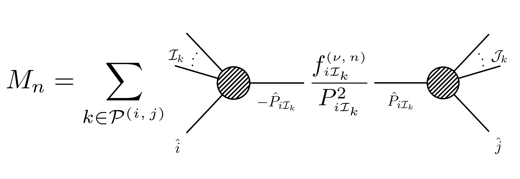
Figure 1: Generalised on-shell recursion relation. This new recursion relation shows the same structure of the usual BCFW one, with a further factor which depends on a sub-set of the zeroes of the amplitude.

The paper is organised as follows. In section 2 we review the BCFW construction both in general and its realisation using the four-dimensional spinor-helicity formalism. In section 3 we discuss the limit of the amplitudes as the momenta are taken to infinity along some complex direction, the degree at which it might diverge, the eventual contribution from the boundary term and their relation with the zeroes of the amplitudes. Here we derive as well the generalised recursion relation. In section 4 we provide the conditions on the channels computed at the location of the zeroes by requiring that our recursion relation satisfies the correct collinear and multi-particle limits. section 5 is dedicated to further comments on the large-$z$ behaviour. In section 6, we work out some examples. Finally, section 7 contains the conclusion and further discussions.

2 BCFW Construction

In the complexified momentum space it is possible to introduce a one-complex parameter deformation such that the deformed momenta satisfy both the on-shell condition and the momentum conservation [3], defining a one-parameter family of amplitudes. This deformation is certainly not unique. The simplest example may be defined by deforming the momenta of just two particles, leaving the others unchanged

$$p^{\mbox{\tiny$(i)$}}(z)\>=\>p^{\mbox{\tiny$(i)$}}-zq,\qquad p^{\mbox{\tiny$(j)$}}(z)\>=\>p^{\mbox{\tiny$(j)$}}+zq,\qquad p^{\mbox{\tiny$(k)$}}(z)\>=\>p^{\mbox{\tiny$(k)$}},$$ (2.1)

where $k$ labels all the particles except for $i$ and $j$. The deformation (2.1) straightforwardly satisfies momentum conservation. The requirement that the deformed momenta are on-shell fixes $q$ to be necessarily complex and such that

$$q^{2}\>=\>0,\qquad p^{\mbox{\tiny$(i)$}}\,\cdot\,q\>=\>0\>=\>p^{\mbox{\tiny$(j)$}}\,\cdot\,q.$$ (2.2)

A deformation of this type defines a one-parameter family of amplitudes $M_{n}(z)$, and it is now possible to analyse the singularity structure of the amplitude as a function of $z$. The poles in $z$ are located in correspondence with the $z$-dependent propagators and they turn out to be all simple poles

$$\frac{1}{\left[P_{\mbox{\tiny$k$}}(z)\right]^{2}}\>=\>\frac{1}{P_{\mbox{\tiny$k$}}^{2}-2z\left(P_{\mbox{\tiny$k$}}\cdot q\right)}\>\Rightarrow\>z_{\mbox{\tiny$k$}}\>=\>\frac{P_{\mbox{\tiny$k$}}^{2}}{2P_{\mbox{\tiny$k$}}\cdot q},$$ (2.3)

where $P_{\mbox{\tiny$k$}}\,=\,\sum_{l\in\mathcal{S}_{k}}p^{\mbox{\tiny$(l)$}}$, $\mathcal{S}_{k}$ is the set of the momenta of the external particles in the $k$-channel, $i\,\in\,\mathcal{S}_{k}$ and $z_{\mbox{\tiny$k$}}$ is the location of the pole. As $z\,\rightarrow\,z_{\mbox{\tiny$k$}}$ the momentum $P_{\mbox{\tiny$k$}}$ in (2.3) goes on-shell and this channel factorises into the product of two on-shell amplitudes

$$M_{n}^{\mbox{\tiny$(i,j)$}}(z)\>\overset{\mbox{\tiny$z\rightarrow z_{\mbox{\tiny$k$}}$}}{\sim}\>\frac{M_{\mbox{\tiny L}}^{\mbox{\tiny$(i,j)$}}(z_{k})M_{\mbox{\tiny R}}^{\mbox{\tiny$(i,j)$}}(z_{k})}{P^{2}_{\mbox{\tiny$k$}}(z)},$$ (2.4)

where the notation $M_{n}^{\mbox{\tiny$(i,j)$}}(z)$ just indicates that the one-parameter family of amplitudes has been obtained by deforming the momenta of the particles labelled by $i$ and $j$. The physical amplitude, which can be obtained from $M_{n}(z)$ by setting $z\,=\,0$, is related to the residues of the poles in (2.4). Let $\mathcal{R}$ be the Riemann sphere obtained as union of the complex plane with the point at infinity $\mathcal{R}\,=\,\mathbb{C}\cup\left\{\infty\right\}$, then

$$0\>=\>\frac{1}{2\pi i}\oint_{\mbox{\tiny$\mathcal{R}$}}\frac{dz}{z}M_{n}^{\mbox{\tiny$(i,j)$}}(z)\>=\>M_{n}(0)-\sum_{k\in\mathcal{P}^{\mbox{\tiny$(i,j)$}}}\frac{M_{\mbox{\tiny L}}^{\mbox{\tiny$(i,j)$}}(z_{k})M_{\mbox{\tiny R}}^{\mbox{\tiny$(i,j)$}}(z_{k})}{P^{2}_{k}}-\mathcal{C}_{n}^{\mbox{\tiny$(i,j)$}}.$$ (2.5)

If $M_{n}^{\mbox{\tiny$(i,j)$}}(z)\,\overset{\mbox{\tiny$z\rightarrow\infty$}}{\rightarrow}0$, the boundary term $\mathcal{C}_{n}^{\mbox{\tiny$(i,j)$}}$ is zero and the solution of eq (2.5) for $M_{n}(0)$ provides with a recursion relation. Such a condition is satisfied by Yang-Mills [3], gravity [5], $\mathcal{N}=4$ Super Yang-Mills and $\mathcal{N}=8$ Supergravity [8], and for amplitudes with external gravitons/gluons, as highest spin particles, under a deformation of the momenta of the gravitons/gluons [7].

2.1 The BCFW Construction and the Spinor-Helicity Formalism

In this section, we briefly introduce the spinor-helicity representation of the scattering amplitudes, that allows to express them as a function of a set of pairs of spinors $\left\{\left(\lambda^{\mbox{\tiny$(i)$}},\,\tilde{\lambda}^{\mbox{\tiny$(i)$}}\right)\right\}$ and of the helicities $\left\{h_{i}\right\}$ of the particles. In four dimensions, this equivalence holds because of the isomorphism $SO(3,1)\,\cong\,SL(2,\mathbb{C})$, which is implemented by the Pauli matrices $\sigma^{\mu}_{a\dot{a}}\,=\,\left(\mathbb{I}_{a\dot{a}},\,\overrightarrow{\sigma}_{a\dot{a}}\right)$:

$$p_{\mu}\quad\longrightarrow\quad p_{a\dot{a}}\>=\>\sigma^{\mu}_{a\dot{a}}p_{\mu}\>=\>\lambda_{a}\tilde{\lambda}_{\dot{a}},$$ (2.6)

with $\lambda_{a}$ and $\tilde{\lambda}_{\dot{a}}$ transforming respectively in the $(1/2,\,0)$ and $(0,\,1/2)$ representation of $SL(2,\mathbb{C})$. In the real momentum space, these two spinors are related by complex conjugation: $\tilde{\lambda}_{\dot{a}}\,=\,\left(\lambda_{a}\right)^{\star}$.

It is possible to define two inner product for spinors, one for each representation of $SL(2,\mathbb{C})$ under which they can transform:

$$\langle\lambda,\,\lambda^{\prime}\rangle\>\equiv\>\epsilon^{ab}\lambda_{a}\lambda^{\prime}_{b},\qquad[\tilde{\lambda},\,\tilde{\lambda}^{\prime}]\>\equiv\>\epsilon^{\dot{a}\dot{b}}\tilde{\lambda}_{\dot{a}}\tilde{\lambda}^{\prime}_{\dot{b}},$$ (2.7)

with $\epsilon_{12}\,=\,1\,=\,\epsilon_{\dot{1}\dot{2}}$, $\epsilon^{12}\,=\,-1\,=\,\epsilon^{\dot{1}\dot{2}}$, and $\epsilon^{ac}\epsilon_{cb}\,=\,\delta^{a}_{\phantom{a}b}$. Notice that the inner products (2.7) are Lorentz invariant.

Assuming the existence of one-particle states and that the Poincaré group acts on scattering amplitudes as it acts on individual states, the helicity operator acts on the amplitudes as follows:

$$\left(\lambda^{\mbox{\tiny$\left(i\right)$}}_{a}\frac{\partial}{\partial\lambda^{\mbox{\tiny$\left(i\right)$}}_{a}}-\tilde{\lambda}^{\mbox{\tiny$\left(i\right)$}}_{\dot{a}}\frac{\partial}{\partial\tilde{\lambda}^{\mbox{\tiny$\left(i\right)$}}_{\dot{a}}}\right)M_{n}\left(1^{\mbox{\tiny$h_{i}$}},\ldots,n^{\mbox{\tiny$h_{i}$}}\right)\>=\>-2h_{i}\,M_{n}\left(1^{\mbox{\tiny$h_{i}$}},\ldots,n^{\mbox{\tiny$h_{i}$}}\right).$$ (2.8)

In the complexified Minkowski space, the isometry group is $SO(3,1,\mathbb{C})\,\cong\,SL(2,\mathbb{C})\,\times\,SL(2,\mathbb{C})$ and each of the two spinors $\lambda_{\mbox{\tiny$a$}}$ and $\tilde{\lambda}_{\mbox{\tiny$\dot{a}$}}$ can be taken to belong to a different copy of $SL(2,\mathbb{C})$, so that they are not related by complex conjugation and, therefore, are independent of each other. Working in the complexified momentum space, the BCFW-deformation (2.1) in terms of the spinors (2.6) turns out to be

$$\tilde{\lambda}^{\mbox{\tiny$(i)$}}(z)\>=\>\tilde{\lambda}^{\mbox{\tiny$(i)$}}-z\tilde{\lambda}^{\mbox{\tiny$(j)$}},\quad\lambda^{\mbox{\tiny$(j)$}}(z)\>=\>\lambda^{\mbox{\tiny$(j)$}}+z{\lambda}^{\mbox{\tiny$(i)$}}.$$ (2.9)

The expression (2.9) actually defines a set of four deformations, which are determined by the sign of the helicities $\left(h_{i},\,h_{j}\right)$ of the deformed particles:

$$\left(h_{i},\,h_{j}\right)\>=\>\left\{\left(-,\,+\right),\left(-,\,-\right),\left(+,\,+\right),\left(+,\,-\right)\right\}.$$ (2.10)

Depending on the helicity configuration (2.10) chosen for the two-particle deformation (2.9), the induced one-parameter family of amplitudes is a different function of $z$ and, therefore, the boundary term $\mathcal{C}_{n}^{\mbox{\tiny$(i,j)$}}$ differs as well.

As mentioned earlier, the helicity-spinor formalism as discussed here is strictly four-dimensional. Generalisations have been proposed in [13, 14, 15] for higher dimensions and in [16] for three-dimensions. Our main results heavily rely on the four-dimensional helicity-spinor formalism. However, as showed in [6], the BCFW-structure of the tree level amplitude is a general feature of a theory and is not related to the dimensionality of the space-time. Therefore, in order to generalise them to dimensions different than four, a little bit of more work needs to be done.

3 The Boundary Term and New Recursion Relations

Let us observe a crucial fact. The one-parameter family of amplitudes $M_{n}^{\mbox{\tiny$(i,j)$}}(z)$ can be written as

$$M_{n}^{\mbox{\tiny$(i,j)$}}(z)\>=\>\sum_{k\in\mathcal{P}^{\mbox{\tiny$(i,j)$}}}\frac{M_{\mbox{\tiny L}}^{\mbox{\tiny$(i,j)$}}(z_{k})M_{\mbox{\tiny R}}^{\mbox{\tiny$(i,j)$}}(z_{k})}{P^{2}_{k}(z)}+\mathcal{C}_{n}^{\mbox{\tiny$(i,j)$}}(z).$$ (3.1)

Since all the singularities located at finite points are contained in the first sum in (3.1), the function $\mathcal{C}_{n}^{\mbox{\tiny$(i,j)$}}(z)$ is just a polynomial in $z$ of order $\nu$:

$$\mathcal{C}_{n}^{\mbox{\tiny$(i,j)$}}(z)\>=\>\mathcal{C}_{n}^{\mbox{\tiny$(i,j)$}}+\sum_{l=1}^{\nu}a_{l}^{\mbox{\tiny$(i,j)$}}z^{l},$$ (3.2)

where $\nu$ is as well the order the amplitude $M_{n}^{\mbox{\tiny$(i,j)$}}(z)$ diverges with, as $z$ is taken to infinity. The zero-th order term in (3.2) is the only one which survives in the integral (2.5) and therefore it is the only contribution to the physical amplitude. Here we are referring to a BCFW-deformation defined as a shift of the momenta of two particles. This is however more general and holds for any type of one-complex parameter deformation.

In order to understand the singularity at infinity, it is instructive to consider the logarithmic derivative of $M_{n}^{\mbox{\tiny$(i,j)$}}(z)$. Its pole structure is just given by simple poles at the location of both the zeroes and the poles of $M_{n}^{\mbox{\tiny$(i,j)$}}(z)$. Furthermore, the residues of such poles correspond to the multiplicity of the zeroes and of the poles of $M_{n}^{\mbox{\tiny$(i,j)$}}(z)$. The BCFW-deformations induce just simple poles at finite locations and, therefore, the residues of the logarithmic derivative with respect to such points is always $-1$. Taking into account the eventual multiplicity of the zeroes, the integration of the logarithmic derivative of $M_{n}^{\mbox{\tiny$(i,j)$}}(z)$ on the Riemann sphere provides with the following equation:

$$0\>=\>\int_{\mathcal{R}}dz\,\frac{M_{n}^{\prime\mbox{\tiny$(i,j)$}}(z)}{M_{n}^{\mbox{\tiny$(i,j)$}}(z)}\>=\>N_{\mbox{\tiny$Z$}}-N_{\mbox{\tiny$P$}}\,\equiv\,N_{\mbox{\tiny$Z$}}^{\mbox{\tiny fin}}-N_{\mbox{\tiny$P$}}^{\mbox{\tiny fin}}-\nu,$$ (3.3)

which is just the generalisation of the argument principle to the Riemann sphere. In (3.3), $N_{\mbox{\tiny$Z$}}$, $N_{\mbox{\tiny$P$}}$, $N_{\mbox{\tiny$Z$}}^{\mbox{\tiny fin}}$, $N_{\mbox{\tiny$P$}}^{\mbox{\tiny fin}}$ and $\nu$ are respectively the number of zeroes (with their multiplicity), the number of poles, the number of zeroes at finite location, the number of poles at finite location, and the multiplicity of the point at infinity. Equation (3.3) relates the latter to $N_{\mbox{\tiny$Z$}}^{\mbox{\tiny fin}}$ and $N_{\mbox{\tiny$P$}}^{\mbox{\tiny fin}}$: $\nu\,=\,N_{\mbox{\tiny$Z$}}^{\mbox{\tiny fin}}-N_{\mbox{\tiny$P$}}^{\mbox{\tiny fin}}$. The number of poles at finite location $N_{\mbox{\tiny$P$}}^{\mbox{\tiny fin}}$ is known for a given theory. Thus, the knowledge of the number of zeroes would fix the large-$z$ behaviour of the amplitudes from first principles.

Let now $\left\{z_{0}^{\mbox{\tiny$(s)$}}\right\}$ be a subset of $n_{\mbox{\tiny$z$}}$ zeroes of the amplitude (3.1) and $\gamma_{0}^{\mbox{\tiny$(s)$}}$ be a contour including just $z_{0}^{\mbox{\tiny$(s)$}}$ and no other zeroes or poles. Using the general expressions (3.1) and (3.2) for the one-parameter family of amplitudes $M_{n}^{\mbox{\tiny$(i,j)$}}(z)$, one obtains the following equations

$$\begin{split}0\>=\>\frac{1}{2\pi i}\oint_{\mbox{\tiny$\gamma_{0}^{(s)}$}}dz\>&\frac{M_{n}^{\mbox{\tiny$(i,j)$}}(z)}{\left(z-z_{0}^{\mbox{\tiny$(s)$}}\right)^{r}}\>=\>\left(-1\right)^{r-1}\sum_{k=1}^{N_{\mbox{\tiny$P$}}^{\mbox{\tiny fin}}}\frac{M_{\mbox{\tiny L}}^{\mbox{\tiny$(i,j)$}}(z_{k})M_{\mbox{\tiny R}}^{\mbox{\tiny$(i,j)$}}(z_{k})}{\left(-2P_{k}\cdot q\right)\left(z_{0}^{\mbox{\tiny$(s)$}}-z_{k}\right)^{r}}+\delta_{\mbox{\tiny$r,1$}}\mathcal{C}_{\mbox{\tiny$n$}}^{\mbox{\tiny$(i,j)$}}+\\ &\hskip 5.69046pt+\sum_{l=1}^{\nu}\frac{l!}{\left(l-r+1\right)!\left(r-1\right)!}a_{l}^{\mbox{\tiny$(i,j)$}}z_{\mbox{\tiny$0$}}^{l-r+1},\quad\mbox{with }\left\{\begin{array}[]{l}r\,=\,1,\ldots,m^{\mbox{\tiny$(s)$}}\\ s\,=\,1,\ldots,n_{z}\end{array}\right.,\end{split}$$ (3.4)

where $m^{\mbox{\tiny$(s)$}}$ is the multiplicity of the zero $z_{0}^{\mbox{\tiny$(s)$}}$. If $n_{z}\,=\,\nu+1$, the system of algebraic equations (3.4) would fix univocally the amplitudes. In particular, the boundary term $\mathcal{C}_{\mbox{\tiny$n$}}^{\mbox{\tiny$\left(i,j\right)$}}$ acquires the form

$$\begin{split}\mathcal{C}_{\mbox{\tiny$n$}}^{\mbox{\tiny$\left(i,j\right)$}}\>&=\>\left(-1\right)^{\nu+1}\sum_{k\in\mathcal{P}^{\mbox{\tiny$(i,j)$}}}\frac{M_{\mbox{\tiny L}}^{\mbox{\tiny$(i,j)$}}(z_{k})M_{\mbox{\tiny R}}^{\mbox{\tiny$(i,j)$}}(z_{k})}{P_{k}^{2}}\left[\prod_{l=1}^{\nu+1}\frac{P_{k}^{2}}{P_{k}^{2}(z_{0}^{\mbox{\tiny$(l)$}})}\right]\times\\ &\times\sum_{l=0}^{\nu}\left(-1\right)^{l}\sum_{\mbox{\tiny$\begin{array}[]{l}r_{1},..,r_{l}\,=\,1\\ r_{1}\neq..\neq r_{l}\end{array}$}}^{\nu+1}\prod_{s=1}^{l}\frac{P_{k}^{2}\left(z_{0}^{\mbox{\tiny$(r_{s})$}}\right)}{P_{k}^{2}}.\end{split}$$ (3.5)

The expression (3.5) determines the boundary term $\mathcal{C}_{\mbox{\tiny$n$}}^{\mbox{\tiny$\left(i,j\right)$}}$ in terms of the lower point on-shell amplitudes! This implies that the presence of the boundary term does not spoil the standard BCFW structure! More precisely, the whole $n$-particle amplitude takes the form

$$M_{n}\>=\>\sum_{k\in\mathcal{P}^{\mbox{\tiny$(i,j)$}}}\left[\frac{M_{\mbox{\tiny L}}^{\mbox{\tiny$(i,j)$}}(\hat{i},\mathcal{I}_{k},-\hat{P}_{\mbox{\tiny$i\mathcal{I}_{k}$}})M_{\mbox{\tiny R}}^{\mbox{\tiny$(i,j)$}}(\hat{P}_{\mbox{\tiny$i\mathcal{I}_{k}$}},\mathcal{J}_{k},\hat{j})}{P_{\mbox{\tiny$i\mathcal{I}_{k}$}}^{2}}\prod_{l=1}^{\nu+1}\left(1-\frac{P_{\mbox{\tiny$i\mathcal{I}_{k}$}}^{2}}{P_{\mbox{\tiny$i\mathcal{I}_{k}$}}^{2}\left(z_{0}^{\mbox{\tiny$(l)$}}\right)}\right)\right],$$ (3.6)

where $\mathcal{I}_{k}$ and $\mathcal{J}_{k}$ are sets of particles such that we have the partition $\left\{i\right\}\cup\left\{j\right\}\cup\mathcal{I}_{k}\cup\mathcal{J}_{k}\,=\,\left\{1,\ldots,n\right\}$, which can contain from $1$ to $n-3$ elements, and the “hat” denotes that the momenta are computed at the location of the pole.

Some comments are in order. As emphasised earlier, even in the presence of the boundary term, a scattering amplitude can be expressed in terms of products of two on-shell scattering amplitudes with fewer external states. The statement that the three-particle amplitudes determine the whole tree level is therefore generalized to any consistent theory of massless particles with a non-trivial S-matrix! More precisely, the amplitudes are determined in terms of the smallest amplitudes defining a particular theory, which may have more external particles than three. However, it is always possible to define effective three-particle amplitudes for such theories, as it was done for $\lambda\phi^{4}$ in [1]. Even if this might not be technically convenient for the actual computation of an amplitude, it anyway points out that the tree-level structure of these theories can be treated on the same footing as the ones for which the three-particle amplitudes are naturally defined.

Furthermore, the number of BCFW channels does not change, and the recursion relation (3.6) can be seen as a “weighted” version of the standard BCFW expression, and the “weight” is given by the term dependent on the location of a subset of zeroes.

Finally, let us point out that the knowledge of a subset of $\nu+1$ zeroes allows us to determine the full structure of the one-parameter family of amplitudes defined by a given BCFW-deformation. In particular, we can explicitly determine as well the leading order in $z$, as $z$ is taken to infinity, which has the interpretation of a hard particle in a soft background [6]

$$a_{\nu}^{\left(i,j\right)}\>=\>(-1)^{\nu+1}\sum_{k\in\mathcal{P}^{\mbox{\tiny$(i,j)$}}}\frac{M_{\mbox{\tiny L}}^{\mbox{\tiny$(i,j)$}}(\hat{i},\mathcal{I}_{k},-\hat{P}_{\mbox{\tiny$i\mathcal{I}_{k}$}})M_{\mbox{\tiny R}}^{\mbox{\tiny$(i,j)$}}(\hat{P}_{\mbox{\tiny$i\mathcal{I}_{k}$}},\mathcal{J}_{k},\hat{j})}{2\,P_{\mbox{\tiny$i\mathcal{I}_{k}$}}\cdot q}\prod_{l=1}^{\nu+1}\frac{2\,P_{\mbox{\tiny$i\mathcal{I}_{k}$}}\cdot q}{P_{\mbox{\tiny$i\mathcal{I}_{k}$}}^{2}\left(z_{0}^{\mbox{\tiny$(l)$}}\right)}.$$ (3.7)

Notice that for $\nu\,=\,0$, i.e. $M_{n}^{\mbox{\tiny$(i,j)$}}(z)\,\overset{z\rightarrow\infty}{\sim}\mathcal{O}\left(1\right)$, the expressions (3.5) for the boundary term and (3.7) for the hard-particle limit coincide, as it should be.

4 Zeroes, UV and Collinear/Multi-particle Limits

In the previous section, we discussed how the knowledge of a subset of zeroes can fix the large-$z$ behaviour of the amplitude under a certain BCFW-deformation, which is given by the difference between the number of zeroes and the number of poles, and the boundary term through their location. The result is the recursion relation (3.6), which shows the same number of terms as the standard BCFW formula.

The question we need to answer now concerns the physical meaning of the location of the zeroes of the amplitudes, or, probably more fruitfully, the physical meaning of the internal propagators when they are evaluated at the location of the zeroes.

Beyond the obvious statement that the location of the zeroes are points in the complexified momentum space where the S-matrix becomes trivial, to our knowledge not much is known about their physical significance. The issue of the zeroes of the complete amplitudes was studied in relation to the analysis of the dispersion relations for the logarithm of the scattering amplitudes [17, 18, 19, 20, 21, 22].

In the present case, the relation (3.6) indeed provides us with a new representation of the full $n$-particle amplitudes for arbitrary theories, and therefore it must provide us with the correct collinear/multi-particle limits. We will show how the zeroes of the amplitudes and its large-$z$ behaviour are fixed by such limits. The collinear/multi-particle channels we will need to analyse can be grouped in the following four classes:

$$\begin{split}&\lim_{\mbox{\tiny$P_{i\mathcal{I}_{k}}^{2}$}\>\rightarrow\>0}P_{\mbox{\tiny$i\mathcal{I}_{k}$}}^{2}\,M_{n}\>=\>M(i,\,\mathcal{I}_{k},\,-P_{i\mathcal{I}_{k}})\,M(P_{i\mathcal{I}_{k}},\mathcal{J}_{k},j),\\ &\lim_{\mbox{\tiny$P_{\mathcal{K}}^{2}$}\>\rightarrow\>0}P_{\mbox{\tiny$\mathcal{K}$}}^{2}\,M_{n}\>=\>M_{s+1}(\mathcal{K},\,-P_{\mathcal{K}})\,M_{n-s+1}(P_{\mathcal{K}},\mathcal{Q},i,j),\\ &\lim_{\mbox{\tiny$P_{k_{1}k_{2}}^{2}$}\>\rightarrow\>0}P_{\mbox{\tiny$k_{1}k_{2}$}}^{2}\,M_{n}\>=\>M_{3}(k_{1},\,k_{2},\,-P_{k_{1}k_{2}})\,M_{n-1}(P_{k_{1}k_{2}},\mathcal{K},i,j),\\ &\lim_{\mbox{\tiny$P_{ij}^{2}$}\>\rightarrow\>0}P_{\mbox{\tiny$ij$}}^{2}\,M_{n}\>=\>M_{3}(i,\,j,\,-P_{ij})\,M_{n-1}(P_{ij},\mathcal{K}),\\ \end{split}$$ (4.1)

where $\mathcal{K}$ in the second line indicates a set of $s\,\geq\,3$ particles and $\mathcal{Q}$ a set of $n-s-2$ particles, so that, together with $\{i\}$ and $\{j\}$, they form the partition $\mathcal{K}\,\cup\,\mathcal{Q}\,\cup\,\left\{i\right\}\,\cup\,\left\{j\right\}\,=\,\left\{1,\ldots,n\right\}$.

Before starting with the discussion of the limits (4.1), it is useful to write down here, for future reference, all the quantities characterising our recursive formula (3.6). As mentioned earlier, the recursive structure (3.6) has been obtained under the deformation (2.1). The induced one-parameter family of amplitudes $M_{\mbox{\tiny$n$}}^{\mbox{\tiny$(i,j)$}}(z)$ shows poles located at

$$z_{\mbox{\tiny$i\mathcal{I}_{k}$}}\>=\>\frac{P_{\mbox{\tiny$i\mathcal{I}_{k}$}}^{2}}{2P_{\mbox{\tiny$i\mathcal{I}_{k}$}}\cdot q}.$$ (4.2)

The amplitudes with fewer external states contained in (3.6) are computed at the locations (4.2), where the deformed momenta have the explicit form

$$\begin{split}&\hat{p}^{\mbox{\tiny$(i)$}}\>\overset{\mbox{\tiny def}}{=}\>p^{\mbox{\tiny$(i)$}}\left(z_{\mbox{\tiny$i\mathcal{I}_{k}$}}\right)\>=\>p^{\mbox{\tiny$(i)$}}-\frac{P_{\mbox{\tiny$i\mathcal{I}_{k}$}}^{2}}{2P_{\mbox{\tiny$i\mathcal{I}_{k}$}}\cdot q}q,\quad\hat{p}^{\mbox{\tiny$(j)$}}\>\overset{\mbox{\tiny def}}{=}\>p^{\mbox{\tiny$(j)$}}\left(z_{\mbox{\tiny$i\mathcal{I}_{k}$}}\right)\>=\>p^{\mbox{\tiny$(j)$}}+\frac{P_{\mbox{\tiny$i\mathcal{I}_{k}$}}^{2}}{2P_{\mbox{\tiny$i\mathcal{I}_{k}$}}\cdot q}q,\\ &\hat{P}_{\mbox{\tiny$i\mathcal{I}_{k}$}}\>\overset{\mbox{\tiny def}}{=}\>P_{\mbox{\tiny$i\mathcal{I}_{k}$}}\left(z_{\mbox{\tiny$i\mathcal{I}_{k}$}}\right)\>=\>P_{\mbox{\tiny$i\mathcal{I}_{k}$}}-\frac{P_{\mbox{\tiny$i\mathcal{I}_{k}$}}^{2}}{2P_{\mbox{\tiny$i\mathcal{I}_{k}$}}\cdot q}q.\end{split}$$ (4.3)

One further comment is in order. Let us explicitly consider the four-dimensional helicity-spinor formalism. In a generic $(k_{1},\,k_{2})$-channel, the limit $P_{\mbox{\tiny$k_{1}k_{2}$}}^{2}\,\rightarrow\,0$ can be taken in two different ways. Specifically, $P_{\mbox{\tiny$k_{1}k_{2}$}}^{2}\,=\,\langle k_{1},\,k_{2}\rangle[k_{1},\,k_{2}]$ with the two Lorentz invariant inner products independent of each other which can therefore be taken to zero in the complexified momentum space, as either $\langle k_{1},\,k_{2}\rangle$ or $[k_{1},\,k_{2}]$ go to zero. This will be of crucial importance in the analysis of the collinear limits of (3.6) and it will be further discussed later.

4.1 The collinear/multi-particle limit $P_{i\mathcal{I}_{k}}^{2}\,\rightarrow\,0$

This limit is manifestly satisfied by the set of recursion relations (3.6) we propose. However, for the sake of completeness, we analyse it in detail. From (4.3), it is easy to see that in this kinematic limit

$$\hat{p}^{\mbox{\tiny$(i)$}}\>\rightarrow\>p^{\mbox{\tiny$(i)$}},\quad\hat{p}^{\mbox{\tiny$(j)$}}\>\rightarrow\>p^{\mbox{\tiny$(j)$}},\quad\hat{P}_{\mbox{\tiny$i\mathcal{I}_{k}$}}\>\rightarrow\>P_{\mbox{\tiny$i\mathcal{I}_{k}$}},$$ (4.4)

so that

$$\lim_{\mbox{\tiny$P_{i\mathcal{I}_{k}}^{2}$}\>\rightarrow\>0}P_{\mbox{\tiny$i\mathcal{I}_{k}$}}^{2}\,M_{n}\>=\>M_{\mbox{\tiny L}}^{\mbox{\tiny$(i,j)$}}(\hat{i},\mathcal{I}_{k},-\hat{P}_{\mbox{\tiny$i\mathcal{I}_{k}$}})M_{\mbox{\tiny R}}^{\mbox{\tiny$(i,j)$}}(\hat{P}_{\mbox{\tiny$i\mathcal{I}_{k}$}},\mathcal{J}_{k},\hat{j}),$$ (4.5)

and

$$\lim_{\mbox{\tiny$P_{i\mathcal{I}_{k}}^{2}$}\>\rightarrow\>0}f_{i\mathcal{I}_{k}}^{\mbox{\tiny$(\nu,n)$}}\,=\,1.$$ (4.6)

Indeed this is not a surprise given that the deformation (2.1) selects all the factorisation channels $P_{i\mathcal{I}_{k}}^{2}\,\rightarrow\,0$ (figure 1).

As emphasised in [23], in the case where either $\mathcal{I}_{k}$ or $\mathcal{J}_{k}$ contains just one particle, the relevant collinear limit is related to only one of the Lorentz invariant spinorial inner products. Specifically, under the deformation (2.9), for $\mathcal{I}_{k}\,=\,\left\{k\right\}$ the relevant singularity is provided by $[i,\,k]\,\longrightarrow\,0$, while for $\mathcal{J}_{k}\,=\,\left\{k\right\}$ by $\langle j,\,k\rangle\,\longrightarrow 0$.

4.2 The multi-particle limit $P_{\mathcal{K}}^{2}\,\rightarrow\,0$

We now consider the factorisation along a class of channels $\mathcal{K}$ which contain at least three particles: $P_{\mathcal{K}}^{2}\,\rightarrow\,0$. In the recursive formula (3.6), let us take $\mathcal{K}$ to be $\mathcal{K}\,=\,\mathcal{K}_{\mathcal{I}}\,\cup\,\mathcal{K}_{\mathcal{J}}$, with $\mathcal{K}_{\mathcal{I}}\,\subseteq\,\mathcal{I}_{k}$ and $\mathcal{K}_{\mathcal{J}}\,\subseteq\,\mathcal{J}_{k}$ - we can think about $\mathcal{I}_{k}$ and $\mathcal{J}_{k}$ as $\mathcal{I}_{k}\,=\,\mathcal{K}_{\mbox{\tiny$\mathcal{I}$}}\,\cup\,\tilde{\mathcal{I}}_{k}$ and $\mathcal{J}_{k}\,=\,\mathcal{K}_{\mbox{\tiny$\mathcal{J}$}}\,\cup\,\tilde{\mathcal{J}}_{k}$. The sum in (3.6) can be split into three classes of terms: $\left(\mathcal{K}_{\mathcal{I}},\,\mathcal{K}_{\mathcal{J}}\right)\,=\,\left\{\left(\mathcal{K},\,\emptyset\right),\,\left(\emptyset,\,\mathcal{K}\right),\,\left(\mathcal{K}_{\mathcal{I}},\,\mathcal{K}_{\mathcal{J}}\right)\right\}$.

Taking the limit $\mathcal{P}_{\mathcal{K}}^{2}\rightarrow 0$, the set of on-shell diagrams $\left(\mathcal{K}_{\mathcal{I}},\,\mathcal{K}_{\mathcal{J}}\right)\,=\,\left(\mathcal{K},\,\emptyset\right)$ shows the singularity $P_{\mathcal{K}}^{2}$ in the sub-amplitude $M_{\mbox{\tiny L}}^{\mbox{\tiny$(i,j)$}}(\hat{i},\mathcal{I}_{k},-\hat{P}_{\mbox{\tiny$i\mathcal{I}_{k}$}})$, which factorises as follows

$$M_{\mbox{\tiny L}}^{\mbox{\tiny$(i,j)$}}(\hat{i},\mathcal{I}_{k},-\hat{P}_{\mbox{\tiny$i\mathcal{I}_{k}$}})\>\overset{\mbox{\tiny$P_{\mathcal{K}}^{2}\,\rightarrow\,0$}}{\longrightarrow}\>M_{s+1}(\mathcal{K},\,-P_{\mathcal{K}})\frac{1}{P_{\mathcal{K}}^{2}}M_{\mbox{\tiny L}}^{\mbox{\tiny$(i,j)$}}(P_{\mathcal{K}},\hat{i},\tilde{\mathcal{I}}_{k},-\hat{P}_{\mbox{\tiny$i\mathcal{I}_{k}$}}).$$ (4.7)

In the second case, $\left(\mathcal{K}_{\mathcal{I}},\,\mathcal{K}_{\mathcal{J}}\right)\,=\,\left(\emptyset,\,\mathcal{K}\right)$, the same type of factorisation occurs in the sub-amplitude $M_{\mbox{\tiny R}}^{\mbox{\tiny$(i,j)$}}(\hat{P}_{\mbox{\tiny$i\mathcal{I}_{k}$}},\mathcal{J}_{k},\hat{j})$:

$$M_{\mbox{\tiny R}}^{\mbox{\tiny$(i,j)$}}(\hat{P}_{\mbox{\tiny$i\mathcal{I}_{k}$}},\mathcal{J}_{k},\hat{j})\>\overset{\mbox{\tiny$P_{\mathcal{K}}^{2}\,\rightarrow\,0$}}{\longrightarrow}\>M_{s+1}(\mathcal{K},\,-P_{\mathcal{K}})\frac{1}{P_{\mathcal{K}}^{2}}M_{\mbox{\tiny R}}^{\mbox{\tiny$(i,j)$}}(P_{\mathcal{K}},\hat{P}_{\mbox{\tiny$i\mathcal{I}_{k}$}},\tilde{\mathcal{J}}_{k},\hat{j})$$ (4.8)

Finally, in the third class of terms neither of the two sub-amplitudes show a singularity in this channel. One might think that the “weight” may show such singularity. However, this cannot be the case given that this condition will not induce this class of terms to factorise and generate a sub-amplitude of type $M_{s+1}(\mathcal{K},\,-P_{\mathcal{K}})$: this would spoil the possibility to recover the correct factorisation properties along this class of channels.

Therefore, (3.6) in the limit $\mathcal{P}_{\mathcal{K}}^{2}\,\rightarrow\,0$ becomes

$$\begin{split}\lim_{\mathcal{P}_{\mathcal{K}}^{2}\,\rightarrow\,0}&\mathcal{P}_{\mathcal{K}}^{2}\,M_{n}\>=\>M_{s+1}(\mathcal{K},\,-P_{\mathcal{K}})\times\\ &\times\left[\sum_{k^{\prime}\in\mathcal{P}^{\mbox{\tiny$(i,j)$}}}\frac{M_{\mbox{\tiny L}}^{\mbox{\tiny$(i,j)$}}(P_{\mathcal{K}},\hat{i},\tilde{\mathcal{I}}_{k^{\prime}},-\hat{P}_{\mbox{\tiny$i\mathcal{I}_{k^{\prime}}$}})M_{\mbox{\tiny R}}^{\mbox{\tiny$(i,j)$}}(\hat{P}_{\mbox{\tiny$i\mathcal{I}_{k^{\prime}}$}},\mathcal{J}_{k^{\prime}},\hat{j})}{P_{\mbox{\tiny$i\mathcal{I}_{k}^{\prime}$}}^{2}}\prod_{l=1}^{\nu+1}\left(1-\frac{P_{\mbox{\tiny$i\mathcal{I}_{k^{\prime}}$}}^{2}}{P_{\mbox{\tiny$i\mathcal{I}_{k^{\prime}}$}}^{2}\left(\bar{z}_{0}^{\mbox{\tiny$(l)$}}\right)}\right)+\right.\\ &\left.+\sum_{k^{\prime\prime}\in\mathcal{P}^{\mbox{\tiny$(i,j)$}}}\frac{M_{\mbox{\tiny L}}^{\mbox{\tiny$(i,j)$}}(\hat{i},\mathcal{I}_{k^{\prime\prime}},-\hat{P}_{\mbox{\tiny$i\mathcal{I}_{k^{\prime\prime}}$}})M_{\mbox{\tiny R}}^{\mbox{\tiny$(i,j)$}}(P_{\mathcal{K}},\hat{P}_{\mbox{\tiny$i\mathcal{I}_{k^{\prime\prime}}$}},\tilde{\mathcal{J}}_{k^{\prime\prime}},\hat{j})}{P_{\mbox{\tiny$i\mathcal{I}_{k^{\prime\prime}}$}}^{2}}\prod_{l=1}^{\nu+1}\left(1-\frac{P_{\mbox{\tiny$i\mathcal{I}_{k^{\prime\prime}}$}}^{2}}{P_{\mbox{\tiny$i\mathcal{I}_{k^{\prime\prime}}$}}^{2}\left(\bar{z}_{0}^{\mbox{\tiny$(l)$}}\right)}\right)\right],\end{split}$$ (4.9)

where $\bar{z}_{0}^{\mbox{\tiny$(l)$}}$ indicates the zero $z_{0}^{\mbox{\tiny$(l)$}}$ in the limit $P_{\mbox{\tiny$\mathcal{K}$}}^{2}\,\rightarrow\,0$, as depicted in figure 2

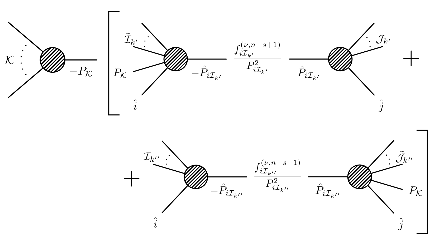
Figure 2: Multi-particle limit $P_{\mathcal{K}}^{2}\,\rightarrow\,0$. In this figure, the behaviour of the terms of the generalised recursion relation (3.6) under the multi-particle limits is depicted. In particular, in the terms contributing, all the particles in the set $\mathcal{K}$ belong to one of the two sub-amplitudes.

Notice that the expression in the square brackets in (4.9) is nothing but our formula (3.6) for an amplitude with fewer external legs! Specifically, if $s\,\geq\,3$ is the number of elements of $\mathcal{K}$, then the term in square brackets in (4.9) represents an on-shell recursion relation for an $(n-s+1)$-particle amplitude. There is one striking feature emerging from (4.9): the large-$z$ (complex-UV) behaviour $\nu$ appearing for the $(n-s+1)$-particle amplitudes is the same as the one for $n$-particles!

One might wonder whether some or all of the terms in the product defining the weights $f_{\mbox{\tiny$i\mathcal{I}_{k}$}}^{\mbox{\tiny$(\nu,n)$}}$ of the $n$-point amplitude goes to one, so that the power with which the $(n-s+1)$-particle amplitudes diverges as $z$ is taken to infinity changes. This is indeed not the case and it will be manifest from the analysis of the collinear limit $P_{ij}^{2}\,\rightarrow\,0$ (section 4.4).

One confusion that might arise from (4.9) is that it might seem to state that the locations of the zeroes for the $n$-particle amplitude and for the $(n-s+1)$-particle amplitudes would coincide. Indeed this should not be the case and it is not implied by (4.9). It simply states that the location of some zeroes of the $(n-s+1)$-particle amplitudes can be obtained as a limit of the one for the zeroes of the $n$-particle amplitude when $P_{\mathcal{K}}^{2}\,\rightarrow\,0$:

$$\lim_{P_{\mathcal{K}}^{2}\,\rightarrow\,0}P_{\mbox{\tiny$i\mathcal{I}_{k}$}}^{2}(z_{0}^{\mbox{\tiny$(l)$}})\>=\>P_{\mbox{\tiny$i\mathcal{I}_{k}$}}^{2}(\bar{z}_{0}^{\mbox{\tiny$(l)$}}),$$ (4.10)

where $\bar{z}_{0}^{\mbox{\tiny$(l)$}}$ is a zero of the $(n-s+1)$-particle amplitude $M_{n-s+1}(i,\,j,\,\mathcal{Q},\,P_{\mbox{\tiny$\mathcal{K}$}})$.

Thinking about the large-$z$ limit as a hard particle of momentum $zq$ propagating in a soft background, this is the statement that the soft particles do not affect the leading (complex) UV behaviour.

4.3 The collinear limit $P_{\mbox{\tiny$k_{1}k_{2}$}}^{2}\,\rightarrow\,0$

In the previous section, we discussed the multi-particle limit $P_{\mathcal{K}}^{2}\,\rightarrow\,0$, with $\mathcal{K}$ containing $s\,\geq\,3$ particles. Here we turn to the two-particle version of this limit, which is more subtle, as pointed out in [23] for gluons and gravitons. However, before starting with the analysis of this collinear limit on the recursion relation (3.6), it is useful to comment on the expected result (third line of equation (4.1)):

$$\lim_{\mbox{\tiny$P_{k_{1}k_{2}}^{2}$}\>\rightarrow\>0}P_{\mbox{\tiny$k_{1}k_{2}$}}^{2}\,M_{n}\>=\>M_{3}(k_{1},\,k_{2},\,-P_{k_{1}k_{2}})\,M_{n-1}(P_{k_{1}k_{2}},\mathcal{K},i,j).$$ (4.11)

As mentioned earlier, there are two possible ways in which the limit $P_{\mbox{\tiny$k_{1}k_{2}$}}^{2}\,\rightarrow\,0$ can be taken. Specifically, considering that $P_{\mbox{\tiny$k_{1}k_{2}$}}^{2}\,=\,\langle k_{1},\,k_{2}\rangle\,[k_{1},\,k_{2}]$ and that the spinors related to the same momentum are independent of each other in the complexified momentum space, it is possible to consider $\langle k_{1},\,k_{2}\rangle\,\rightarrow\,0$ or $[k_{1},\,k_{2}]\,\rightarrow\,0$. In the case, $\langle k_{1},\,k_{2}\rangle\,\rightarrow\,0$, the holomorphic spinors in the three-particle amplitude on the right-hand-side of (4.11) are proportional to each other, so that $M_{3}(k_{1},\,k_{2},\,-P_{k_{1}k_{2}})$ is just a function of the anti-holomorphic spinors [1] for theories with three-particle $\delta$-derivative interactions, with $\delta\,>\,0$. Similarly, when the anti-holomorphic inner product $[k_{1},\,k_{2}]$ is taken to zero, the three-particle amplitude is just function of the holomorphic spinors (again, for theories with three-particle $\delta$-derivative interactions, with $\delta\,>\,0$).

Let us analyze the expected factorisation (4.11) in both complex collinear limits, starting with theories with three-particle $\delta$-derivative interactions ($\delta\,>\,0$). As $\langle k_{1},\,k_{2}\rangle\,\rightarrow\,0$, $\lambda^{\mbox{\tiny$(k_{1})$}}\,\sim\,\lambda^{\mbox{\tiny$(k_{2})$}}$ and the momentum $P_{k_{1}k_{2}}$ may acquire the form

$$\begin{split}P_{k_{1}k_{2}}\>\overset{\mbox{\tiny def}}{=}\>\lambda^{\mbox{\tiny$(k_{1})$}}\tilde{\lambda}^{\mbox{\tiny$(k_{1})$}}+\lambda^{\mbox{\tiny$(k_{2})$}}\tilde{\lambda}^{\mbox{\tiny$(k_{2})$}}\>&\overset{\mbox{\tiny$\langle k_{1},\,k_{2}\rangle\,\rightarrow\,0$}}{\longrightarrow}\lambda^{\mbox{\tiny$(k_{1})$}}\left(\tilde{\lambda}^{\mbox{\tiny$(k_{1})$}}+\frac{\langle k_{2},\,\mu\rangle}{\langle k_{1},\,\mu\rangle}\tilde{\lambda}^{\mbox{\tiny$(k_{2})$}}\right),\\ &\overset{\mbox{\tiny$\langle k_{1},\,k_{2}\rangle\,\rightarrow\,0$}}{\longrightarrow}\lambda^{\mbox{\tiny$(k_{2})$}}\left(\frac{\langle k_{1},\,\mu\rangle}{\langle k_{2},\,\mu\rangle}\tilde{\lambda}^{\mbox{\tiny$(k_{1})$}}+\tilde{\lambda}^{\mbox{\tiny$(k_{2})$}}\right),\end{split}$$ (4.12)

for some reference spinor $\mu$. The two expressions in (4.12) depend on whether the holomorphic spinor $\lambda^{\mbox{\tiny$(k_{1}k_{2})$}}$ of $P_{k_{1}k_{2}}$ is chosen to be $\lambda^{\mbox{\tiny$(k_{1})$}}$ or $\lambda^{\mbox{\tiny$(k_{2})$}}$. One has indeed the freedom to relate $\lambda^{\mbox{\tiny$(k_{1}k_{2})$}}$ to $\lambda^{\mbox{\tiny$(k_{1})$}}$ or $\lambda^{\mbox{\tiny$(k_{2})$}}$ through proportionality factors different from one, at the price of changing the other proportionality factors in front of the anti-holomorphic spinors in (4.12). Let us choose the following identification

$$\lambda^{\mbox{\tiny$(k_{1}k_{2})$}}\>=\>\lambda^{\mbox{\tiny$(k_{1})$}},\qquad\tilde{\lambda}^{\mbox{\tiny$(k_{1}k_{2})$}}\>=\>\tilde{\lambda}^{\mbox{\tiny$(k_{1})$}}+\frac{\langle k_{2},\,\mu\rangle}{\langle k_{1},\,\mu\rangle}\tilde{\lambda}^{\mbox{\tiny$(k_{2})$}}.$$ (4.13)

The three-particle amplitude on the right-hand-side of (4.11) becomes

$$\begin{split}M_{3}&(k_{1}^{\mbox{\tiny$h_{1}$}},\,k_{2}^{\mbox{\tiny$h_{2}$}},\,-P_{k_{1}k_{2}}^{\mbox{\tiny$h_{12}$}})\>=\\ &=\>\kappa_{\mbox{\tiny$1-\delta$}}[k_{1},\,k_{2}]^{\mbox{\tiny$-(h_{12}-h_{1}-h_{2})$}}[k_{2},\,P_{k_{1}k_{2}}]^{-(h_{1}-h_{2}-h_{12})}[P_{k_{1}k_{2}},\,k_{1}]^{-(h_{2}-h_{12}-h_{1})}\>=\\ &=\>\kappa_{\mbox{\tiny$1-\delta$}}(-1)^{2h_{1}+2h_{2}}[k_{1},\,k_{2}]^{\delta}\left(\frac{\langle k_{1},\,\mu\rangle}{\langle k_{2},\,\mu\rangle}\right)^{2h_{2}-\delta},\end{split}$$ (4.14)

where the subscript in the coupling constant indicates the dimensionality of the coupling constant itself and we used the fact that the number of derivatives $\delta$ of the three-particle interaction is related to the helicities of the particles in a anti-holomorphic three-particle amplitude through the relation $\delta\,=\,h_{1}+h_{2}+h_{12}$ [1].

The case $[k_{1},\,k_{2}]\,\rightarrow\,0$ is treated similarly, with the spinorial representation of $P_{k_{1}k_{2}}$ obtained from (4.12) and (4.13) by exchanging holomorphic and anti-holomorphic spinors, and the three-particle amplitude acquires the form

$$\begin{split}M_{3}&(k_{1}^{\mbox{\tiny$h_{1}$}},\,k_{2}^{\mbox{\tiny$h_{2}$}},\,-P_{k_{1}k_{2}}^{\mbox{\tiny$h_{12}$}})\>=\\ &=\>\kappa_{\mbox{\tiny$1-\delta$}}\langle k_{1},\,k_{2}\rangle^{\mbox{\tiny$h_{12}-h_{1}-h_{2}$}}\langle k_{2},\,P_{k_{1}k_{2}}\rangle^{h_{1}-h_{2}-h_{12}}\langle P_{k_{1}k_{2}},\,k_{1}\rangle^{h_{2}-h_{12}-h_{1}}\>=\\ &=\>\kappa_{\mbox{\tiny$1-\delta$}}(-1)^{2h_{1}+2h_{2}}\langle k_{1},\,k_{2}\rangle^{\delta}\left(\frac{[k_{2},\,\mu]}{[k_{1},\,\mu]}\right)^{2h_{2}+\delta},\end{split}$$ (4.15)

where we used the relation $\delta\,=\,-h_{1}-h_{2}-h_{12}$ which characterises the holomorphic three-particle amplitude.

Notice that if we restrict ourselves to a theory with $\delta$-derivative three-particle interactions only, as we are doing, the helicity of $P_{k_{1}k_{2}}$ is univocally fixed by the relations $\delta\,=\,-h_{1}-h_{2}-h_{12}$, if the three-particle amplitude is function of the holomorphic spinors only, or $\delta\,=\,h_{1}+h_{2}+h_{12}$ if it is just a function of the anti-holomorphic spinors.

In the case of $\delta\,=\,0$, the helicity of $P_{k_{1}k_{2}}$ is fixed to be $h_{12}\,=\,-h_{1}-h_{2}$ and the general form of $M_{3}(k_{1}^{\mbox{\tiny$h_{1}$}},\,k_{2}^{\mbox{\tiny$h_{2}$}},\,-P_{k_{1}k_{2}}^{\mbox{\tiny$h_{12}$}})$ is

$$\begin{split}M_{3}&(k_{1}^{\mbox{\tiny$h_{1}$}},\,k_{2}^{\mbox{\tiny$h_{2}$}},\,-P_{k_{1}k_{2}}^{\mbox{\tiny$h_{12}$}})\>=\\ &=\>\kappa_{\mbox{\tiny H}}\frac{\langle k_{2},\,P_{k_{1}k_{2}}\rangle^{2h_{1}}\langle P_{k_{1}k_{2}},\,k_{1}\rangle^{2h_{2}}}{\langle k_{1},\,k_{2}\rangle^{2h_{1}+2h_{2}}}+\kappa_{\mbox{\tiny A}}\frac{[k_{1},\,k_{2}]^{2h_{1}+2h_{2}}}{[k_{2},\,P_{k_{1}k_{2}}]^{2h_{1}}[P_{k_{1}k_{2}},\,k_{1}]^{2h_{2}}}.\end{split}$$ (4.16)

In the limits $\langle k_{1},\,k_{2}\rangle\,\rightarrow\,0$ and $[k_{1},\,k_{2}]\,\rightarrow\,0$, the above expression reads

$$\begin{split}&\left.M_{3}(k_{1}^{\mbox{\tiny$h_{1}$}},\,k_{2}^{\mbox{\tiny$h_{2}$}},\,-P_{k_{1}k_{2}}^{\mbox{\tiny$h_{12}$}})\right|_{\mbox{\tiny$\langle k_{1},\,k_{2}\rangle\,\rightarrow\,0$}}\>=\>\hat{\kappa}(-1)^{2h_{1}+2h_{2}}\left(\frac{\langle k_{1},\,\mu\rangle}{\langle k_{2},\,\mu\rangle}\right)^{2h_{2}},\\ &\left.M_{3}(k_{1}^{\mbox{\tiny$h_{1}$}},\,k_{2}^{\mbox{\tiny$h_{2}$}},\,-P_{k_{1}k_{2}}^{\mbox{\tiny$h_{12}$}})\right|_{\mbox{\tiny$[k_{1},\,k_{2}]\,\rightarrow\,0$}}\>=\>\hat{\kappa}(-1)^{2h_{1}+2h_{2}}\left(\frac{[k_{2},\,\mu]}{[k_{1},\,\mu]}\right)^{2h_{2}},\end{split}$$ (4.17)

with $\hat{\kappa}\,=\,\kappa_{\mbox{\tiny H}}+\kappa_{\mbox{\tiny A}}$ being the effective three-particle coupling.

Now we are ready to analyse these complex collinear limits on the recursive relation (3.6). As in section 4.2, there are three classes of terms to analyse and we will do it in the next subsections.

4.3.1 Particles $k_{1}$ and $k_{2}$ on the same sub-amplitude

First, let us focus on the case in which $k_{1}$ and $k_{2}$ belong to the same sub-amplitude and take the limit $[k_{1},k_{2}]\,\rightarrow\,0$. The analysis follows the one in the section 4.2 as long as $\tilde{\mathcal{I}}_{k}$ and $\tilde{\mathcal{J}}_{k}$ are not empty. If $k_{1},\,k_{2}\,\in\,\mathcal{I}_{k}$ and $\tilde{\mathcal{I}}_{k}\,=\,\emptyset$, the sub-amplitude $M_{\mbox{\tiny L}}^{\mbox{\tiny$(i,j)$}}(\hat{i},\mathcal{I}_{k},-\hat{P}_{\mbox{\tiny$i\mathcal{I}_{k}$}})$ is a four-particle amplitude with channels $P_{\hat{i}k_{1}}^{2}$, $P_{\hat{i}k_{2}}^{2}$ and $P_{k_{1}k_{2}}^{2}$. It turns out that $\hat{\tilde{\lambda}}^{(i)}\propto\tilde{\lambda}^{(k_{1})}\propto\tilde{\lambda}^{(k_{2})}$ and therefore all the channels do contribute. The amplitude $M_{\mbox{\tiny L}}^{\mbox{\tiny$(i,j)$}}(\hat{i},\mathcal{I}_{k},-\hat{P}_{\mbox{\tiny$i\mathcal{I}_{k}$}})$ therefore factorises as:

$$\begin{split}M_{\mbox{\tiny L}}^{\mbox{\tiny$(i,j)$}}(\hat{i},\mathcal{I}_{k},-\hat{P}_{\mbox{\tiny$i\mathcal{I}_{k}$}})\>&\equiv\>M_{\mbox{\tiny L}}^{\mbox{\tiny$(i,j)$}}(\hat{i},k_{1},k_{2},-\hat{P}_{\mbox{\tiny$ik_{1}k_{2}$}})\>\overset{\mbox{\tiny$P_{k_{1}k_{2}}^{2}\,\rightarrow\,0$}}{\longrightarrow}\\ &\overset{\mbox{\tiny$P_{k_{1}k_{1}}^{2}\,\rightarrow\,0$}}{\longrightarrow}\>M_{3}(k_{1},k_{2},-P_{\mbox{\tiny$k_{1}k_{2}$}})\frac{1}{P_{\mbox{\tiny$k_{1}k_{2}$}}^{2}}M_{\mbox{\tiny L}}^{\mbox{\tiny$(i,j)$}}(P_{\mbox{\tiny$k_{1}k_{2}$}},\hat{i},-\hat{P}_{\mbox{\tiny$i(k_{1}k_{2})$}})+\\ &\hskip 14.22636pt+M_{3}(\hat{i},k_{1},-P_{\hat{i}k_{1}})\frac{1}{P_{\hat{i}k_{1}}^{2}}M_{3}(P_{\hat{i}k_{1}},k_{2},-P_{\hat{i}(k_{1}k_{2})})+\\ &\hskip 14.22636pt+M_{3}(\hat{i},k_{2},-P_{\hat{i}k_{2}})\frac{1}{P_{\hat{i}k_{2}}^{2}}M_{3}(P_{\hat{i}k_{2}},k_{1},-P_{\hat{i}(k_{1}k_{2})}),\end{split}$$ (4.18)

where the brackets in the notation $P_{i(k_{1}k_{2})}$ indicate that the momentum $p^{\mbox{\tiny$(k_{1})$}}+p^{\mbox{\tiny$(k_{2})$}}$ is on-shell in this limit, and the following identifications are understood: $\tilde{\lambda}^{(k_{1}k_{2})}\,=\,\tilde{\lambda}^{(k_{1})}$ and $\tilde{\lambda}^{(k_{2})}\,=\,\frac{[k_{2},\mu]}{[k_{1},\mu]}\tilde{\lambda}^{(k_{1})}$. In (4.18) we wrote all the possible channels. Notice that for a $\delta$-derivative interaction $(\delta\,>\,0)$, one of the two three-point amplitudes in each of the terms on the r.h.s side of (4.18) has to be anti-holomorphic. However, all the momenta in these three-particle amplitudes are characterised by having the anti-holomorphic spinors proportional to each other. As a consequence, such terms are always zero.

In the case of $0$-derivative interactions, instead, both the holomorphic and anti-holomorphic term of a three-particle amplitude are relevant and all the terms in (4.18) turn out to be non-zero.

As far as the factor $f_{i\mathcal{I}_{k}}^{(\nu,n)}$ is concerned, it is easy to see that in these cases the same condition (4.10) holds, while the factors $f_{ik_{1}}^{(\nu,n)}$ and $f_{ik_{2}}^{(\nu,n)}$ are such that

$$\lim_{[k_{1},k_{2}]\rightarrow 0}f_{i\bar{k}}^{(\nu,n)}\>\equiv\>\lim_{[k_{1},\,k_{2}]\,\rightarrow\,0}\prod_{l=1}^{\nu+1}\left(1-\frac{P_{i\bar{k}}^{2}}{P_{i\bar{k}}^{2}(z_{0}^{(l)})}\right)\>=\>\prod_{l=1}^{\nu+1}\left(1-\frac{P_{i(k_{1}k_{2})}^{2}}{P_{i(k_{1}k_{2})}^{2}(\bar{z}_{0}^{(l)})}\right)\>\equiv\>f_{i(k_{1}k_{2})}^{(\nu,n-1)},$$ (4.19)

where $\bar{z}_{0}$ indicates the zeroes of the lower point amplitudes and $\bar{k}\,\in\,\{k_{1},\,k_{2}\}$.

The same reasoning applies in the case $k_{1},\,k_{2}\,\in\,\mathcal{J}_{k}$ and $\tilde{\mathcal{J}}_{k}\,=\,\emptyset$ as $\langle k_{1},\,k_{2}\rangle\rightarrow 0$.

4.3.2 Particles $k_{1}$ and $k_{2}$ on different sub-amplitudes

Another difference with respect to the case analysed in section 4.2 lies on the fact that, in the present case, the class of terms $\left(\mathcal{K}_{\mbox{\tiny$\mathcal{I}$}},\mathcal{K}_{\mbox{\tiny$\mathcal{J}$}}\right)\,\neq\,\left(\emptyset,\emptyset\right)$ does contribute. Specifically, such a class of terms contains all those diagrams such that $\left(\mathcal{K}_{\mbox{\tiny$\mathcal{I}$}},\mathcal{K}_{\mbox{\tiny$\mathcal{J}$}}\right)\,=\,\left(k_{1},k_{2}\right)$ or $\left(\mathcal{K}_{\mbox{\tiny$\mathcal{I}$}},\mathcal{K}_{\mbox{\tiny$\mathcal{J}$}}\right)\,=\,\left(k_{2},k_{1}\right)$. Obviously, the treatment of these two sub-cases is equivalent and related by relabelling $k_{1}\,\leftrightarrow\,k_{2}$. Here we can further distinguish three sub-classes of diagrams:

$$\left(\tilde{\mathcal{I}}_{k},\tilde{\mathcal{J}}_{k}\right)\,=\,\left\{\left(\tilde{\mathcal{I}}_{k},\emptyset\right),\,\left(\emptyset,\tilde{\mathcal{J}}_{k}\right),\left(\tilde{\mathcal{I}}_{k},\tilde{\mathcal{J}}_{k}\right)\right\}.$$ (4.20)

The last case is analogous to the $\left(\mathcal{K}_{\mbox{\tiny$\mathcal{I}$}},\mathcal{K}_{\mbox{\tiny$\mathcal{J}$}}\right)$ one in section 4.2: for these diagrams $P_{\mbox{\tiny$k_{1}k_{2}$}}^{2}\,\rightarrow\,0$ does not appear as a singularity.

As far as the other two sub-classes of terms are concerned, they are characterised by the presence of three-particle amplitudes: $M_{\mbox{\tiny R}}^{\mbox{\tiny$(i,j)$}}(\hat{P}_{\mbox{\tiny$i\mathcal{I}_{k}$}},\bar{k},\hat{j})$ for $\left(\tilde{\mathcal{I}}_{k},\tilde{\mathcal{J}}_{k}\right)\,=\,\left(\tilde{\mathcal{I}}_{k},\emptyset\right)$, and $M_{\mbox{\tiny L}}^{\mbox{\tiny$(i,j)$}}(\hat{i},\bar{k},-\hat{P}_{\mbox{\tiny$i\mathcal{I}_{k}$}})$ for $\left(\tilde{\mathcal{I}}_{k},\tilde{\mathcal{J}}_{k}\right)\,=\,\left(\emptyset,\tilde{\mathcal{J}}_{k}\right)$, where $\bar{k}\,\in\,\left\{k_{1},\,k_{2}\right\}$. This implies that, for each of these two classes, there are two contributions and they are such that $\bar{k}\,\cdot\,\hat{P}_{\mbox{\tiny$i\mathcal{I}_{k}$}}\,=\,0$.

For the case $\left(\tilde{\mathcal{I}}_{k},\tilde{\mathcal{J}}_{k}\right)\,=\,\left(\tilde{\mathcal{I}}_{k},\emptyset\right)$, the BCFW-deformation on the spinors is provided in (2.9), and the spinors evaluated at the location of the pole $z_{j\bar{k}}\,=\,-\langle j,\bar{k}\rangle/\langle i,\bar{k}\rangle$ are given by

$$\begin{split}&\hat{\tilde{\lambda}}^{\mbox{\tiny$(i)$}}\>=\>\tilde{\lambda}^{\mbox{\tiny$(i)$}}+\frac{\langle j,\bar{k}\rangle}{\langle i,\bar{k}\rangle}\tilde{\lambda}^{\mbox{\tiny$(j)$}},\qquad\hat{\lambda}^{\mbox{\tiny$(j)$}}\>=\>\lambda^{\mbox{\tiny$(j)$}}-\frac{\langle j,\bar{k}\rangle}{\langle i,\bar{k}\rangle}\lambda^{\mbox{\tiny$(i)$}}\,=\,\frac{\langle i,j\rangle}{\langle i,\bar{k}\rangle}\lambda^{\mbox{\tiny$(\bar{k})$}},\\ &-\hat{P}_{\mbox{\tiny$i\mathcal{I}_{k}$}}\>\equiv\>\hat{P}_{j\bar{k}}\>=\>P_{j\bar{k}}-\frac{\langle j,\bar{k}\rangle}{\langle i,\bar{k}\rangle}\lambda^{\mbox{\tiny$(i)$}}\tilde{\lambda}^{\mbox{\tiny$(j)$}}\>=\>\lambda^{\mbox{\tiny$(\bar{k})$}}\left(\tilde{\lambda}^{\mbox{\tiny$(\bar{k})$}}+\frac{\langle i,j\rangle}{\langle i,\bar{k}\rangle}\tilde{\lambda}^{\mbox{\tiny$(j)$}}\right).\end{split}$$ (4.21)

For theories with $\delta$-derivative three-particle interaction ($\delta\,>\,0$), the proportionality among the holomorphic spinors in $M_{\mbox{\tiny R}}^{\mbox{\tiny$(i,j)$}}(\hat{P}_{\mbox{\tiny$i\mathcal{I}_{k}$}},k_{2},\hat{j})$ implies that it is expressed just in terms of the anti-holomorphic spinors [1]. For theories with $0$-derivative three-particle interaction ($\delta\,=\,0$), both the holomorphic and anti-holomorphic term in the three-particle amplitudes are non-zero [1] and the effective three-particle coupling constant is just a linear combination of the holomorphic and anti-holomorphic ones, as showed earlier.

The limit $\langle k_{1},\,k_{2}\rangle\>\longrightarrow\>0$ induces a singularity in the sub-amplitude $M_{\mbox{\tiny L}}^{\mbox{\tiny$(i,j)$}}(\hat{i},\tilde{k},\tilde{\mathcal{I}}_{k},-\hat{P}_{i\mathcal{I}_{k}})$:

$$\begin{split}&\frac{1}{\left(p^{\mbox{\tiny$(k_{1})$}}+\hat{P}_{jk_{2}}\right)^{2}}\>=\>\frac{1}{\langle k_{1},\,k_{2}\rangle\left([k_{1},k_{2}]+\frac{\langle i,j\rangle}{\langle i,k_{2}\rangle}[k_{1},j]\right)},\\ &\frac{1}{\left(p^{\mbox{\tiny$(k_{2})$}}+\hat{P}_{jk_{1}}\right)^{2}}\>=\>\frac{1}{\langle k_{2},\,k_{1}\rangle\left([k_{2},k_{1}]+\frac{\langle i,j\rangle}{\langle i,k_{1}\rangle}[k_{2},j]\right)}.\end{split}$$ (4.22)

Notice that in the limit $\langle k_{1},\,k_{2}\rangle\>\longrightarrow\>0$, the holomorphic spinors for $p^{(\tilde{k})}$ and $\hat{P}_{j\bar{k}}$ are proportional to each other, with $\tilde{k}\,\in\,\{k_{1},\,k_{2}\}$ and $\tilde{k}\,\neq\,\bar{k}$. This channel does not instead show a singularity in the limit $[k_{1},\,k_{2}]\>\longrightarrow\>0$. Repeating the same argument on the term characterised by $\left(\tilde{\mathcal{I}}_{k},\tilde{\mathcal{J}}_{k}\right)\,=\,\left(\emptyset,\tilde{\mathcal{J}}_{k}\right)$, it turns out to be singular as $[k_{1},\,k_{2}]\>\longrightarrow\>0$ rather than in the limit $\langle k_{1},\,k_{2}\rangle\>\longrightarrow\>0$.

Therefore, in the limit $P_{\mbox{\tiny$k_{1}k_{2}$}}^{2}\,\rightarrow\,0$, the sub-amplitudes $M_{\mbox{\tiny L}}^{\mbox{\tiny$(i,j)$}}(\hat{i},\tilde{k},\tilde{\mathcal{I}}_{k},-\hat{P}_{i\mathcal{I}_{k}})$ and
$M_{\mbox{\tiny R}}^{\mbox{\tiny$(i,j)$}}(\hat{P}_{i\mathcal{I}_{k}},\tilde{k},\tilde{\mathcal{J}}_{k},\hat{j})$ factorise as follows

$$\begin{split}&M_{\mbox{\tiny L}}^{\mbox{\tiny$(i,j)$}}(\hat{i},\tilde{k},\tilde{\mathcal{I}}_{k},\hat{P}_{j\bar{k}})\>\overset{\langle k_{1},k_{2}\rangle\rightarrow 0}{\longrightarrow}\>M_{3}(\tilde{k},\hat{P}_{\mbox{\tiny$j\bar{k}$}},-P_{\mbox{\tiny$\tilde{k}(\hat{j}\bar{k})$}})\frac{1}{P_{\mbox{\tiny$\tilde{k}(\hat{j}\bar{k}$)}}^{2}}M_{\mbox{\tiny L}}^{\mbox{\tiny$(i,j)$}}(P_{\mbox{\tiny$\tilde{k}(\hat{j}\bar{k})$}},\hat{i},\tilde{\mathcal{I}}_{k})\\ &M_{\mbox{\tiny R}}^{\mbox{\tiny$(i,j)$}}(\hat{P}_{i\bar{k}},\tilde{k},\tilde{\mathcal{J}}_{k},\hat{j})\>\overset{[k_{1},k_{2}]\rightarrow 0}{\longrightarrow}\>M_{3}(\tilde{k},\hat{P}_{\mbox{\tiny$i\bar{k}$}},-P_{\mbox{\tiny$\tilde{k}(\hat{i}\bar{k})$}})\frac{1}{P_{\mbox{\tiny$\tilde{k}\hat{P}_{i\bar{k}}$}}^{2}}M_{\mbox{\tiny R}}^{\mbox{\tiny$(i,j)$}}(P_{\mbox{\tiny$\tilde{k}(\hat{i}\bar{k})$}},\tilde{\mathcal{J}}_{k},\hat{j}).\end{split}$$ (4.23)

As far as the factor $f_{i\mathcal{I}_{k}}^{(\nu,n)}$ is concerned, it is easy to see that in the above limits one has

$$\begin{split}&\lim_{\langle k_{1},\,k_{2}\rangle\,\rightarrow\,0}f_{j\bar{k}}^{(\nu,n)}\>\equiv\>\lim_{\langle k_{1},\,k_{2}\rangle\,\rightarrow\,0}\prod_{l=1}^{\nu+1}\left(1-\frac{P_{j\bar{k}}^{2}}{P_{j\bar{k}}^{2}(z_{0}^{(l)})}\right)\>=\>\prod_{l=1}^{\nu+1}\left(1-\frac{P_{j(k_{1}k_{2})}^{2}}{P_{j(k_{1}k_{2})}^{2}(\bar{z}_{0}^{(l)})}\right)\>\equiv\>f_{j(k_{1}k_{2})}^{(\nu,n-1)},\\ &\lim_{[k_{1},\,k_{2}]\,\rightarrow\,0}f_{i\bar{k}}^{(\nu,n)}\>\equiv\>\lim_{[k_{1},\,k_{2}]\,\rightarrow\,0}\prod_{l=1}^{\nu+1}\left(1-\frac{P_{i\bar{k}}^{2}}{P_{i\bar{k}}^{2}(z_{0}^{(l)})}\right)\>=\>\prod_{l=1}^{\nu+1}\left(1-\frac{P_{i(k_{1}k_{2})}^{2}}{P_{i(k_{1}k_{2})}^{2}(\bar{z}_{0}^{(l)})}\right)\>\equiv\>f_{i(k_{1}k_{2})}^{(\nu,n-1)},\end{split}$$ (4.24)

where $\bar{z}_{0}^{(l)}$ indicates a zero of an $(n-1)$-particle amplitude. We will comment in more detail on this in the next subsection.

4.3.3 Factorisation in the collinear limit $P_{k_{1}k_{2}}^{2}\,\rightarrow\,0$

In the previous subsections, we discussed the behaviour of the different classes of terms in the generalised on-shell representation as the limit $P_{k_{1}k_{2}}^{2}\,\rightarrow\,0$ is taken. Using this knowledge let us now see explicitly how the correct factorisation property is reproduced.

First of all, let us notice that the $(n-1)$-particle amplitude in (4.11) can be expressed via the on-shell representation (3.6). For the case of theories with $0$-derivative interactions, it is easy to see that all terms in (4.11) are correctly reproduced by the classes of terms for $M_{n}$ discussed in the subsection 4.3.1. More precisely, such classes contain extra-terms, which are of the type of the ones in second and third lines of (4.18). This means that, together with the terms discussed in subsection 4.3.2, they need to add up to zero, which is straightforward to check, with a little algebra.

For theories with $\delta$-derivative interactions $(\delta\,>\,0)$, the on-shell representation (3.6) of the $n$-point amplitude gets a vanishing contribution from terms where the two particles $k_{1}$ and $k_{2}$ belong to the same sub-amplitude and such sub-amplitude is a four-particle amplitude. However, expressing the $(n-1)$-amplitude in (4.11) through the recursion relation (3.6), the r.h.s. of (4.11) actually shows such type of contributions. This means that they should be reproduced by the terms discussed in subsection 4.3.2. In the limit $[k_{1},k_{2}]\,\rightarrow\,0$:

$$\begin{split}&M_{3}^{\mbox{\tiny H}}\left(k_{1},k_{2},-P_{k_{1}k_{2}}\right)M_{3}^{\mbox{\tiny H}}\left(\hat{i},P_{k_{1}k_{2}},-\hat{P}_{i(k_{1}k_{2})}\right)\frac{f_{i(k_{1}k_{2})}^{\mbox{\tiny$(\nu,n-1)$}}}{P_{i(k_{1}k_{2})}^{2}}M_{n-2}\left(\hat{P}_{i(k_{1}k_{2})},\mathcal{K},\hat{j}\right)\>=\\ &=\>\lim_{[k_{1},k_{2}]\rightarrow 0}\left[M_{3}^{\mbox{\tiny H}}\left(\hat{i},k_{1},-\hat{P}_{ik_{1}}\right)\frac{f_{ik_{1}}^{\mbox{\tiny$(\nu,n)$}}}{P_{ik_{1}}^{2}}M_{3}^{\mbox{\tiny H}}\left(\hat{P}_{ik_{1}},k_{2},-P_{(\hat{i}k_{1})k_{2}}\right)\frac{\langle k_{1},k_{2}\rangle}{\langle k_{1},k_{2}\rangle+\frac{[j,i]}{[j,k_{1}]}\langle i,k_{2}\rangle}\times\right.\\ &\hskip 28.45274pt\times\left.M_{n-2}\left(P_{(\hat{i}k_{1})k_{2}},\mathcal{K},\hat{j}\right)+\left(k_{1}\>\longleftrightarrow\>k_{2}\right)\right],\end{split}$$ (4.25)

where we used the notation $M_{3}^{\mbox{\tiny H}}$ to emphasise that these three-particle amplitudes are functions of the holomorphic spinors only (figure 3).

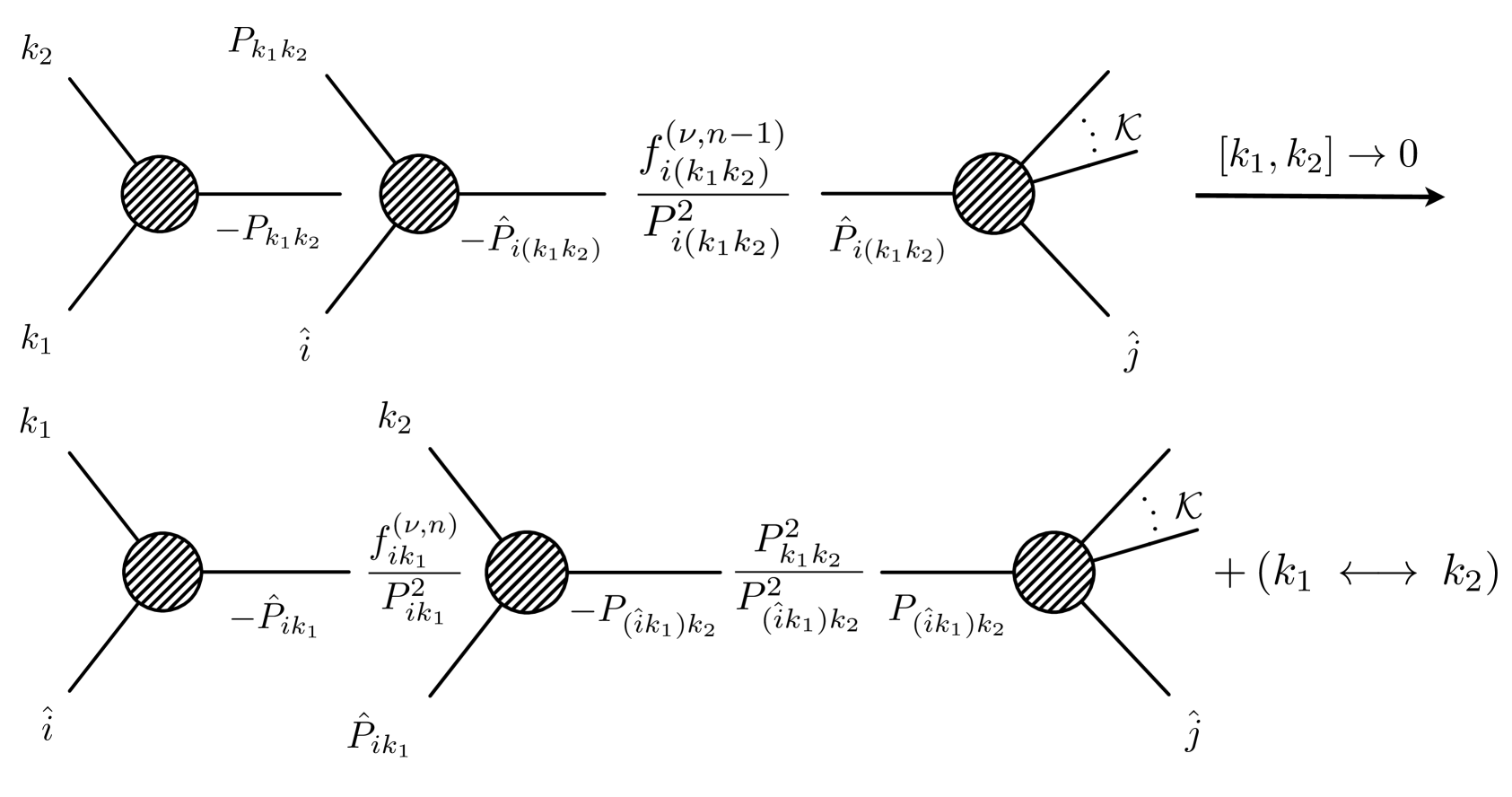
Figure 3: Collinear limit $P_{k_{1}k_{2}}^{2}\,\rightarrow\,0$. For theories with $\delta$-derivative interactions ($\delta\,>\,0$), the analysis of this collinear limit returns a non-trivial equality which, for theories with internal quantum numbers, gives the algebra of the internal group (4.25) and (4.26)

.

Notice that, in such a limit, $P_{(\hat{i}k_{1})k_{2}}\,\equiv\,\hat{P}_{i(k_{1}k_{2})}$ and, as discussed earlier, $f_{i\bar{k}}^{\mbox{\tiny$(\nu,n)$}}\,\rightarrow\,f_{i(k_{1}k_{2})}^{\mbox{\tiny$(\nu,n-1)$}}$. As a consequence, one can factor out $f_{ik_{1}k_{2}}^{\mbox{\tiny$(\nu,n)$}}M_{n-2}\left(\hat{P}_{i(k_{1}k_{2})},\mathcal{K},\hat{j}\right)$ in (4.25). With a little of algebra, such a relation can be written as

$$\begin{split}\varepsilon_{\mbox{\tiny$k_{1}k_{2}a$}}\varepsilon_{\mbox{\tiny$iaP$}}(-1)^{2h_{i}}&\left(1+\frac{[k_{2},\mu]}{[k_{1},\mu]}\frac{\langle i,k_{2}\rangle}{\langle k_{1},k_{2}\rangle}\right)^{\delta-1}=\varepsilon_{\mbox{\tiny$ik_{1}a$}}f_{\mbox{\tiny$ak_{2}P$}}(-1)^{2h_{2}}\left(1+\frac{[j,i]}{[j,k_{1}]}\frac{\langle i,k_{2}\rangle}{\langle k_{1},k_{2}\rangle}\right)^{\delta-1}+\\ &+\varepsilon_{\mbox{\tiny$ik_{2}a$}}\varepsilon_{\mbox{\tiny$ak_{1}P$}}(-1)^{2h_{1}+1}\left(\frac{[j,i]}{[j,k_{1}]}\frac{\langle i,k_{2}\rangle}{\langle k_{1},k_{2}\rangle}+\frac{[k_{2},\mu]}{[k_{1},\mu]}\frac{\langle i,k_{2}\rangle}{\langle k_{1},i\rangle}\right)^{\delta-1},\end{split}$$ (4.26)

where we allowed for the possibility of internal quantum numbers by introducing the structure constants $\varepsilon$’s, $\kappa\,\rightarrow\,\kappa\varepsilon_{abc}$, and a sum for the repeated indices is understood. In case there is no internal symmetry, one can set them to $1$. One can check in both cases how this relation is satisfied by fixing the theory, i.e. the helicities of the particles involved $\{h_{i},h_{1},h_{2}\}$ and the number of the derivative in the three-particle interaction.

The analysis of the limit $\langle k_{1},k_{2}\rangle\rightarrow 0$ proceeds along the same lines.

4.4 The collinear limit $P_{ij}^{2}\,\rightarrow\,0$

A great deal of information is provided by the $\left(i,j\right)$-channel, which does not appear explicitly in (3.6). As discussed in [23] for scattering of gluons and gravitons, in the standard BCFW-representation this singularity appears as a soft singularity, when the deformed momenta of either particle-$i$ or particle-$j$ vanishes. We will show how requiring the correct factorisation in this channel fixes the complex-UV behaviour as well as it provides conditions on the zeroes. As for the $(k_{1},\,k_{2})$-channel, we analyse the limits $[i,\,j]\,\rightarrow\,0$ and $\langle i,\,j\rangle\,\rightarrow\,0$ separately.

Let us start with $[i,\,j]\,\rightarrow\,0$. In this limit, the amplitude should factorise as follows

$$\lim_{\mbox{\tiny$[i,j]$}\>\rightarrow\>0}P_{\mbox{\tiny$ij$}}^{2}\,M_{n}\>=\>M_{3}(i,\,j,\,-P_{ij}^{h_{ij}})\,M_{n-1}(P_{ij}^{-h_{ij}},\mathcal{K}),$$ (4.27)

with $h_{ij}\,=\,-h_{i}-h_{j}-\delta$. For future reference, it is convenient to write down here the explicit expression for the three-particle amplitude in (4.27):

$$M_{3}(i,\,j,\,-P_{ij}^{h_{ij}})\>=\>\kappa_{1-\delta}\left(-1\right)^{2(h_{i}+h_{j})}\langle i,j\rangle^{\delta}\left(\frac{[i,\mu]}{[j,\mu]}\right)^{2h_{i}+\delta},$$ (4.28)

where we used the fact that, in this limit, the on-shell momentum $P_{ij}$ can be written as

$$P_{ij}\,=\,\left(\frac{[i,\mu]}{[j,\mu]}\lambda^{(i)}+\lambda^{(j)}\right)\tilde{\lambda}^{(j)},$$ (4.29)

with the identifications

$$\tilde{\lambda}^{(i)}\>\overset{\mbox{\tiny def}}{=}\>\frac{[i,\mu]}{[j,\mu]}\tilde{\lambda}^{(j)},\quad\lambda^{(ij)}\>\overset{\mbox{\tiny def}}{=}\>\frac{[i,\mu]}{[j,\mu]}\lambda^{(i)}+\lambda^{(j)},\quad\tilde{\lambda}^{(ij)}\>\overset{\mbox{\tiny def}}{=}\>\tilde{\lambda}^{(j)},$$ (4.30)

and $\tilde{\lambda}^{(\mu)}$ being some reference spinor. The expression for the three-particle amplitude (4.28) is valid for any $\delta\,\geq\,0$.

It is easy to see that the only terms of the recursion relation which can contribute are (see figure 4)

$$\lim_{\mbox{\tiny$[i,\,j]\,\rightarrow\,0$}}P_{ij}^{2}\,M_{n}\>=\>\lim_{\mbox{\tiny$[i,\,j]\,\rightarrow\,0$}}P_{ij}^{2}\sum_{k}M_{3}(\hat{i},\,k,\,-\hat{P}_{ik}^{h_{ik}})\frac{f_{ik}^{\mbox{\tiny$(\nu,n)$}}}{P_{ik}^{2}}M_{n-1}(\hat{P}_{ik}^{-h_{ik}},\,\mathcal{J}_{k},\,\hat{j}),$$ (4.31)

where $h_{ik}\,=\,-h_{i}-h_{k}-\delta$, the poles are $z_{ik}\,=\,[i,\,k]/[j,\,k]$ and the relevant quantities computed at the location of the poles are

$$\hat{\tilde{\lambda}}^{\mbox{\tiny(i)}}\>=\>\frac{[j,i]}{[j,k]}\tilde{\lambda}^{\mbox{\tiny(k)}},\quad\hat{\lambda}^{\mbox{\tiny(j)}}\>=\>\lambda^{\mbox{\tiny(j)}}+\frac{[i,k]}{[j,k]}\lambda^{\mbox{\tiny(i)}},\quad\hat{P}_{ik}\>=\>p^{\mbox{\tiny$(k)$}}+\frac{[j,i]}{[j,k]}\lambda^{\mbox{\tiny(i)}}\tilde{\lambda}^{\mbox{\tiny(k)}}.$$ (4.32)

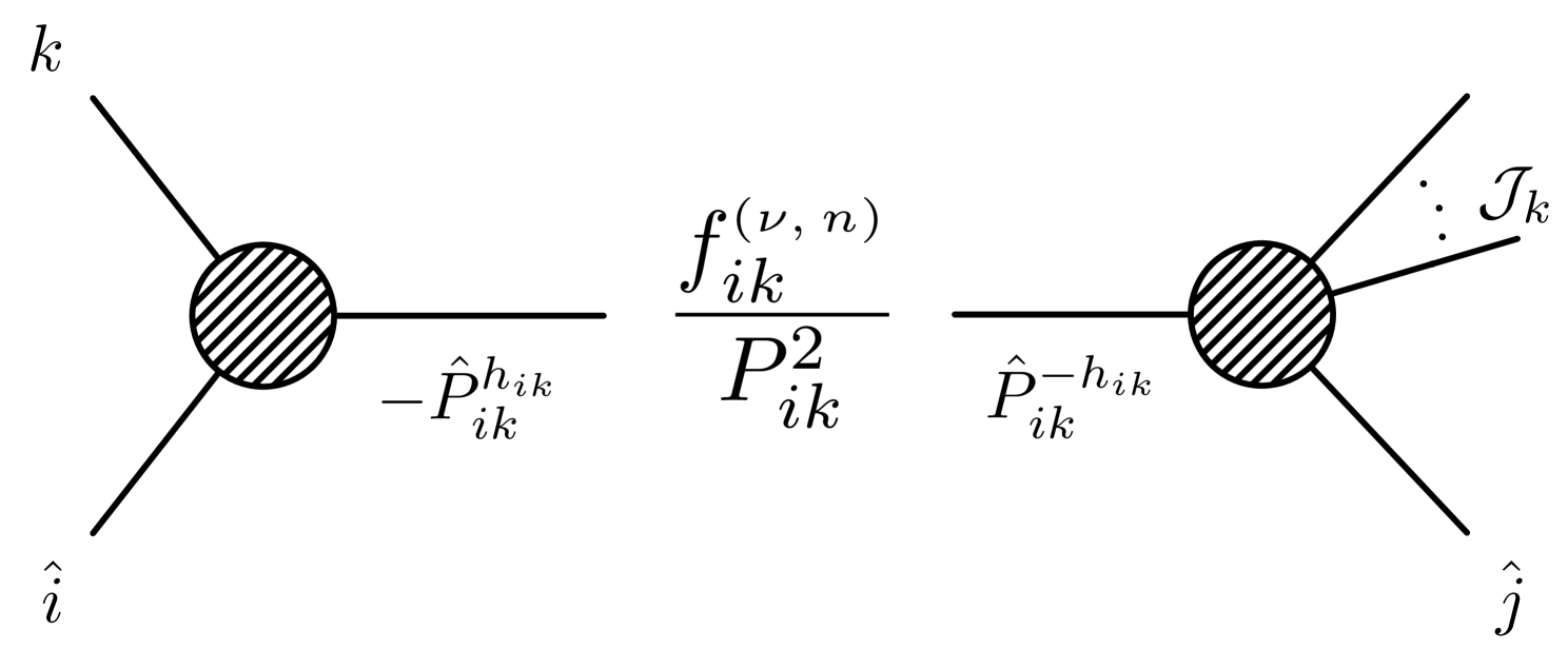
Figure 4: Collinear limit $[i,j]\,\rightarrow\,0$. There are just one class of terms contributing to this limit, which is characterised by a three-particle amplitude of type $M_{3}\left(\hat{i},k,-\hat{P}_{ij}\right)$.

From (4.32), one can notice that the limit $[i,j]\,\rightarrow\,0$ implies that $\hat{\tilde{\lambda}}^{\mbox{\tiny$(i)$}}$, and consequently the momentum of particle-$i$, vanishes, as well as $\hat{p}^{\mbox{\tiny$(j)$}}\,\rightarrow\,P_{ij}$ and $\hat{P}_{ik}\,\rightarrow\,p^{\mbox{\tiny$(k)$}}$. A further consequence is that all the $(n-1)$-particle amplitudes in the sum (4.31) are mapped into $M_{n-1}\left(P_{ij}^{h_{j}},p_{k}^{-h_{ik}},\mathcal{J}_{k}\right)$. There is an important subtlety. This $(n-1)$-particle amplitude has exactly the same momenta for the external states as the one in (4.27), but with the fundamental difference that, generically, the helicities carried by the states with momenta $P_{ij}$ and $p_{k}$ are not the same as the states with same momenta in (4.27). However, it is always possible to relate these amplitudes by a dimensionless factor:

$$M_{n-1}\left(P_{ij}^{h_{j}},p_{k}^{-h_{ik}},\mathcal{J}_{k}\right)\>=\>\mathcal{H}_{n-1}^{(k)}M_{n-1}(P_{ij}^{-h_{ij}},\mathcal{K}),$$ (4.33)

with $\mathcal{H}_{n-1}^{(k)}\,=\,1$ if $h_{ij}\,=\,-h_{j}$ and $h_{ik}\,=\,-h_{k}$. Beyond being dimensionless, this factor can depend in an helicity-blind way on the spinors of the particles in $\mathcal{J}_{k}$ and it has to show the proper helicity scaling with the spinors of $P_{ij}$ and $p_{k}$. Using the relation (4.33), the $(n-1)$-particle amplitude can be factored out from the sum (4.31), leaving in the sum the factor $\mathcal{H}_{n-1}^{(k)}$, which can be computed explicitly for a given theory. Let us now focus on the three-particle amplitudes $M_{3}(\hat{i},\,k,\,-\hat{P}_{ik}^{h_{ik}})$, which can be explicitly written as

$$M_{3}(\hat{i},\,k,\,-\hat{P}_{ik}^{h_{ik}})\>=\>\mathcal{\kappa}_{1-\delta}(-1)^{2(h_{i}+h_{k})}\langle i,k\rangle^{\delta}\left(\frac{[j,i]}{[j,k]}\right)^{2h_{i}+\delta}.$$ (4.34)

From (4.28), (4.33) and (4.34), eq (4.31) becomes

$$\begin{split}\lim_{\mbox{\tiny$[i,\,j]\,\rightarrow\,0$}}P_{ij}^{2}\,M_{n}\>=\>&\left[\lim_{[i,j]\rightarrow 0}\sum_{k}(-1)^{2(h_{j}+h_{k})}\left(\frac{\langle i,k\rangle}{\langle i,j\rangle}\right)^{\delta-1}\left(\frac{[j,i]}{[j,k]}\frac{[j,\mu]}{[i,\mu]}\right)^{2h_{i}+\delta}\frac{[i,j]}{[i,k]}f_{ik}^{(\nu,n)}\mathcal{H}_{n-1}^{(k)}\right]\times\\ &\times M_{3}\left(i,j,-P_{ij}\right)M_{n-1}(P_{ij},\mathcal{K}).\end{split}$$ (4.35)

The above expression reproduces the correct factorisation property (4.27) if and only if the term in square brackets is one. Let us now analyse it in some detail. First of all, one notices the presence of the factor $[i,j]^{2h_{i}+\delta+1}$.

If $2h_{i}+\delta+1\,>\,0$, the requirement of $f_{ik}^{(\nu,n)}$ to be proportional to some negative power of $[i,j]$ needs necessarily to hold in order to reproduce the correct factorisation properties.

Let us now look at the explicit expression for $f_{ik}^{\mbox{\tiny$(\nu,n)$}}$ when $\nu\,\geq\,0$. Unitarity, through the requirement for the amplitude to factorise properly, implies that

$$P_{ik}^{2}(z_{0}^{\mbox{\tiny$(l)$}})\>\equiv\>\langle i,k\rangle\left([i,k]-z_{0}^{\mbox{\tiny$(l)$}}[j,k]\right)\>=\>\langle i,k\rangle\alpha_{ik}^{\mbox{\tiny$(l)$}}[i,j],$$ (4.36)

and, consequently, $f_{ik}^{\mbox{\tiny$(\nu,n)$}}$ with $\nu\,\geq\,0$ becomes

$$\begin{split}f_{ik}^{\mbox{\tiny$(\nu,n)$}}\>&\equiv\>\prod_{l=1}^{\nu+1}\left(1-\frac{P_{ik}^{2}}{P_{ik}^{2}(z_{0}^{\mbox{\tiny$(l)$}})}\right)\>\equiv\>(-1)^{\nu+1}\left(\prod_{l=1}^{\nu+1}\frac{P_{ik}^{2}}{P_{ik}^{2}(z_{0}^{\mbox{\tiny$(l)$}})}\right)\prod_{l=1}^{\nu+1}\left(1-\frac{P_{ik}^{2}(z_{0}^{\mbox{\tiny$(l)$}})}{P_{ik}^{2}}\right)\>=\\ &=\>(-1)^{\nu+1}\left(\frac{[i,k]}{[i,j]}\right)^{\nu+1}\left(\prod_{l=1}^{\nu+1}\alpha_{ik}^{\mbox{\tiny$(l)$}}\right)^{-1}\prod_{l=1}^{\nu+1}\left(1-\alpha_{ik}^{\mbox{\tiny$(l)$}}\frac{[i,j]}{[i,k]}\right).\end{split}$$ (4.37)

From (4.37), the collinear limit (4.35) can be conveniently written as

$$\begin{split}\lim_{\mbox{\tiny$[i,\,j]\,\rightarrow\,0$}}P_{ij}^{2}\,M_{n}\>=\>&\left[\lim_{[i,j]\rightarrow 0}\sum_{k}(-1)^{\xi}\left(\frac{\langle i,k\rangle}{\langle i,j\rangle}\right)^{\delta-1}\left(\frac{[i,k]}{[j,k]}\frac{[j,\mu]}{[i,\mu]}\right)^{2h_{i}+\delta}\left(\frac{[i,j]}{[i,k]}\right)^{2h_{i}+\delta-\nu}\frac{\mathcal{H}_{n-1}^{(k)}}{\prod_{l=1}^{\nu+1}\alpha_{ik}^{\mbox{\tiny$(l)$}}}\right]\times\\ &\times M_{3}\left(i,j,-P_{ij}\right)M_{n-1}(P_{ij},\mathcal{K}),\end{split}$$ (4.38)

where $\xi\,=\,2(h_{i}+h_{j}+h_{k})+\delta+\nu+1$. Notice that, in this limit, the term in the second round-brackets in (4.38) is actually one. Thus, the correct factorisation requirement in the $(i,j)$-channel can be finally written as

$$\lim_{[i,j]\rightarrow 0}\sum_{k}(-1)^{2(h_{i}+h_{j}+h_{k})+\delta+\nu+1}\left[\left(\frac{\langle i,k\rangle}{\langle i,j\rangle}\right)^{\delta-1}\left(\frac{[i,j]}{[i,k]}\right)^{2h_{i}+\delta-\nu}\frac{\mathcal{H}_{n-1}^{(k)}}{\prod_{l=1}^{\nu+1}\alpha_{ik}^{\mbox{\tiny$(l)$}}}\right]\>=\>1.$$ (4.39)

The condition (4.39) univocally fixes $\nu$, and therefore the large-$z$ behaviour of the amplitudes, for a given theory:

$$\nu\,=\,2h_{i}+\delta+m,$$ (4.40)

where $m$ can be one or zero, depending on the fact that the sum (4.35) generates or not one extra factor of $[i,j]$. However, in order to check whether this might or might not be the case, one would need to look at specific theories. It is important to point out that one can see that such an extra factor does not depend on the number $n$ of the external states. Furthermore, the large-$z$ behaviour $\nu$ depends just on the helicities of the particles whose momenta have been deformed as well as on the number of derivatives of the three-particle interactions.

If, instead, $2h_{i}+\delta+1\,\leq\,0$, the term in square brackets in (4.35) is finite and different from zero for $f_{ik}^{(\nu,n)}\,=\,1$, i.e. the standard BCFW recursion relation holds. Thus the helicity of particle-$i$ - whose anti-holomorphic spinor has been deformed - needs to be negative in any case. Just to confirm this, let us discuss the behaviour of the amplitude as $[i,j]\,\rightarrow\,0$ and $h_{i}$ is positive. There are two cases to take into consideration which are related to the two possible $2$-particle deformations: $\left(h_{i},h_{j}\right)\,=\,\left\{\left(+,+\right),\left(+,-\right)\right\}$.

For $\delta\,>\,0$, in the first case no factorisation should occur and indeed this is the case given that the eventual three-particle amplitude in (4.27) would have to be anti-holomorphic and, therefore, vanishing in the limit $[i,j]\,\rightarrow\,0$. In the second case, instead, the correct factorisation is not reproduced. This just implies that the standard BCFW recursion relation does not hold and $\nu\,\geq\,0$. Notice, in fact, that the momenta deformation (2.9) with helicities $\left(h_{i},h_{j}\right)\,=\,\left(+,-\right)$ is what in the literature has been referred to as “wrong shift”. In such a case, the correct factorisation is reproduced if and only if the “weight” $f_{ik}^{\mbox{\tiny$(\nu,n)$}}$ is proportional to some negative power of $[i,j]$ in such a way to cancel the $[i,j]$-term in the numerator.

For theories with $0$-derivative three-particle interactions, in both cases the factorisation is allowed, meaning that, as before, $f_{ik}^{\mbox{\tiny$(\nu,n)$}}$ needs to be proportional to some negative power of $[i,j]$ and, therefore, $\nu\,\geq\,0$.

Following the same arguments above, one can discuss the holomorphic limit $\langle i,j\rangle\,\rightarrow\,0$ (figure 5), obtaining the conditions

$$\begin{split}&\hskip 128.0374ptP_{jk}^{2}(z_{0}^{\mbox{\tiny$(l)$}})\>=\>\langle i,j\rangle\alpha_{jk}^{\mbox{\tiny$(l)$}}[j,k],\\ &\lim_{\langle i,j\rangle\rightarrow 0}\sum_{k}(-1)^{2(h_{i}+h_{j}+h_{k})+\delta+\nu+1}\left[\left(\frac{[k,j]}{[i,j]}\right)^{\delta-1}\left(\frac{\langle i,j\rangle}{\langle j,k\rangle}\right)^{\delta-2h_{j}-\nu}\frac{\tilde{\mathcal{H}}_{n-1}^{(k)}}{\prod_{l=1}^{\nu+1}\alpha_{jk}^{\mbox{\tiny$(l)$}}}\right]\>=\>1,\end{split}$$ (4.41)

and the factor $\tilde{\mathcal{H}}_{n-1}^{(k)}$ is defined analogously to $\mathcal{H}_{n-1}^{(k)}$ in (4.33).

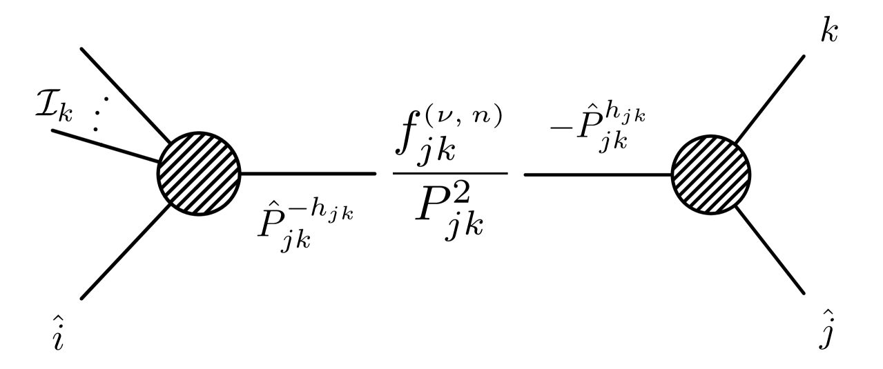
Figure 5: Collinear limit $\langle i,j\rangle\,\rightarrow\,0$. There are just one class of terms contributing to this limit, which is characterised by a three-particle amplitude of type $M_{3}\left(\hat{P}_{ij},k,\hat{j}\right)$.

Notice that two conditions (4.39) and (4.41) do not need to hold simultaneously since a given theory may factorise just under one of the two limits.

Summarising, the analysis of the $P_{ij}^{2}\,\rightarrow\,0$ limit shows that the the large-$z$ behaviour is independent of the number of external states and it depends only on the characteristics of the interactions and on the helicities of the deformed particles.

4.5 Collinear/Multi-particle limits and zeroes of the amplitudes: a Summary

In the previous subsections we have seen how unitarity, through the analysis of the collinear/multi-particle limits, fixes conditions on the zeroes of the amplitudes or, more precisely, on the Lorentz invariants computed at the location of the zeroes. For the sake of clarity, it is suitable to summarise here these conditions:

$$\begin{split}&\hskip 71.13188ptP_{ik}^{2}(z_{0}^{\mbox{\tiny$(l)$}})\>=\>\langle i,k\rangle\alpha_{ik}^{\mbox{\tiny$(l)$}}[i,j],\qquad P_{jk}^{2}(z_{0}^{\mbox{\tiny$(l)$}})\>=\>\langle i,j\rangle\alpha_{jk}^{\mbox{\tiny$(l)$}}[j,k],\\ &\hskip 71.13188pt\lim_{P_{\mathcal{K}}^{2}\rightarrow 0}f_{\mbox{\tiny$i\mathcal{I}_{k}$}}^{\mbox{\tiny$(\nu,\,n)$}}\>=\>f_{\mbox{\tiny$i\mathcal{I}_{k}$}}^{\mbox{\tiny$(\nu,\,n-s+1)$}},\qquad\lim_{P_{i\mathcal{I}_{k}}^{2}\rightarrow 0}f_{i\mathcal{I}_{k}}^{\mbox{\tiny$(\nu,n)$}}\,=\,1,\\ &\hskip 71.13188pt\lim_{[k_{1},k_{2}]\rightarrow 0}f_{\mbox{\tiny$i\bar{k}$}}^{\mbox{\tiny$(\nu,n)$}}\>=\>f_{\mbox{\tiny$i(k_{1}k_{2})$}}^{\mbox{\tiny$(\nu,n-1)$}},\qquad\lim_{\langle k_{1},k_{2}\rangle\rightarrow 0}f_{\mbox{\tiny$j\bar{k}$}}^{\mbox{\tiny$(\nu,n)$}}\>=\>f_{\mbox{\tiny$j(k_{1}k_{2})$}}^{\mbox{\tiny$(\nu,n-1)$}},\\ &\lim_{[i,j]\rightarrow 0}\sum_{k}(-1)^{2(h_{i}+h_{j}+h_{k})+\delta+\nu+1}\left[\left(\frac{\langle i,k\rangle}{\langle i,j\rangle}\right)^{\delta-1}\left(\frac{[i,j]}{[i,k]}\right)^{2h_{i}+\delta-\nu}\frac{\mathcal{H}_{n-1}^{(k)}}{\prod_{l=1}^{\nu+1}\alpha_{ik}^{\mbox{\tiny$(l)$}}}\right]\>=\>1,\\ &\lim_{\langle i,j\rangle\rightarrow 0}\sum_{k}(-1)^{2(h_{i}+h_{j}+h_{k})+\delta+\nu+1}\left[\left(\frac{[k,j]}{[i,j]}\right)^{\delta-1}\left(\frac{\langle i,j\rangle}{\langle j,k\rangle}\right)^{\delta-2h_{j}-\nu}\frac{\tilde{\mathcal{H}}_{n-1}^{(k)}}{\prod_{l=1}^{\nu+1}\alpha_{jk}^{\mbox{\tiny$(l)$}}}\right]\>=\>1.\end{split}$$ (4.42)

Some comments are now in order. The collinear/multi-particle limits relate as well the “weight” factors $f_{\mbox{\tiny$i\mathcal{I}_{k}$}}^{\mbox{\tiny$(\nu,n)$}}$ to the ones of amplitudes with fewer external states through the relations (4.42). This is a hint that it should be possible to reconstruct such factors from the ones of smaller amplitudes. In some cases, such a connection driven by (4.42) is obvious and we will discuss them in section 6. However, one would like to formalise a consistent procedure to find it. Even if some attempts, e.g. looking at a second BCFW-deformation, seemed to point towards the correct direction, so far we did not succeed and we leave it for future work. The existence of such a connection would imply that the last two relations in (4.42) for the four-particle amplitudes would univocally fix the “weights” $f_{\mbox{\tiny$i\mathcal{I}_{k}$}}^{\mbox{\tiny$(\nu,n)$}}$ for any $n$. These relations are easy to solve in the case of four particles, and lead to the following conditions on the zeroes [24]:

$$\prod_{r=1}^{N_{P}^{\mbox{\tiny fin}}}P_{r}^{2}(z_{0}^{\mbox{\tiny$(l)$}})\>=\>(-1)^{N_{P}^{\mbox{\tiny fin}}}\left(P_{ij}^{2}\right)^{N_{P}^{\mbox{\tiny fin}}},$$ (4.43)

where $N_{P}^{\mbox{\tiny fin}}$ is the number of BCFW-poles, $P_{r}^{2}(z_{0}^{\mbox{\tiny$(l)$}})$ is the Mandelstam variable related to the pole $r$ and evaluated at the location of the zero $z_{0}^{\mbox{\tiny$(l)$}}$.

5 More on the complex-UV limit

In section 4.4 we have seen how the large-$z$ behaviour for the amplitudes can be determined by the analysis of the collinear limit $P_{ij}^{2}\,\rightarrow\,0$ and is independent of the number of external states. A more extensive discussion about this is in order.

Already in [23], it was noticed that the correct collinear singularity in the $(i,j)$-channel emerges in the BCFW construction as a soft singularity $\hat{p}^{\mbox{\tiny$(i)$}}\,\rightarrow\,0$ or $\hat{p}^{\mbox{\tiny$(j)$}}\,\rightarrow\,0$ and, moreover, that the standard BCFW recursion relations were failing when this soft singularity was not enough to reproduce the correct factorisation property in this channel.

The analysis in [23] as well as the one in this paper point out a connection between the soft limits for the deformed particles / factorisation in the $(i,j)$-channel and the large-$z$ behaviour. In section 4.4, we showed how the large-$z$ behaviour is fixed just in terms of the number of derivatives of the particular interaction and the helicities of the deformed particles. The same exact analysis, which is valid for arbitrary $n$, can be done for amplitudes which satisfy standard BCFW recursion relations. Conditions of the type of those in the last two lines in (4.42) link the helicities of the deformed particles to the number of derivatives in the three-particle interactions. Specifically,

$$h_{i}\,=\,-\frac{\delta+1+m}{2}\quad\mbox{and/or}\quad h_{j}\,=\,\frac{\delta+1+m}{2},$$ (5.1)

where $m$ can be one or zero, depending on the fact that the sum of the terms contributing in the $P_{ij}^{2}\,\rightarrow\,0$ generates or not one extra factor of $[i,j]$ or $\langle i,j\rangle$.

6 Examples

In this section we apply the generalised on-shell recursion relations (3.6) and the conditions (4.42) for constructing the scattering amplitudes for a number of examples.

6.1 Gluon scattering amplitudes: “wrong” deformation

It is well known that there are three classes of deformations (2.9) under which the standard BCFW recursion relations are valid for gluon scattering amplitudes:

$$(h_{i},h_{j})\,=\,\left\{(-,+),\,(-,-),\,(+,+)\right\}.$$

A further possibility for the choice of the helicities $(h_{i},\,h_{j})\,=\,(+,-)$ leads the deformed amplitude $M_{n}^{\mbox{\tiny$(i,j)$}}$ not to vanish as $z\,\rightarrow\,0$. Using the recursion relations (3.6), we reconstruct the gluons amplitudes through the “wrong” deformation. This issue was discussed in [11], where the boundary term for gluon amplitudes has been obtained through on-shell recursion relations from $\mathcal{N}=4$ Super Yang-Mills.

6.1.1 MHV amplitudes

Let us start with the simplest example, the MHV gluon $n$-particle scattering amplitude $M_{n}(1^{-},2^{+},3^{-},4^{+},\ldots,n^{+})$, using the deformation

$$\lambda^{(1)}(z)\>=\>\lambda^{(1)}+z\lambda^{(2)},\qquad\tilde{\lambda}^{(2)}(z)\>=\>\tilde{\lambda}^{(2)}-z\tilde{\lambda}^{(1)}.$$ (6.1)

The on-shell representation induced by (6.1) shows just one pole at the location $z_{1n}\,=\,-\langle 1,n\rangle/\langle 2,n\rangle$ and it has the following form

$$M_{n}\>=\>M_{3}(\hat{1}^{-},n^{+},-\hat{P}_{1n}^{+})\frac{f^{\mbox{\tiny$(\nu,n)$}}_{1n}}{P_{1n}^{2}}M_{n-1}(\hat{P}_{1n}^{-},(n-1)^{+},\ldots,4^{+},3^{-},\hat{2}^{+}).$$ (6.2)

First of all, the large-$z$ behaviour is obtained through the condition in the last line of (4.42). Being characterised by just on term, the correct factorisation property as $\langle 1,2\rangle\,\rightarrow\,0$ is obtained for $\nu\,=\,\delta-2h_{1}\,=\,3$ and it is possible to see that there is just one zero of multiplicity $4$. Furthermore, the factor $\mathcal{H}_{n-1}$ is given by $\langle n,3\rangle^{4}/\langle P_{12},3\rangle^{4}$ and it has this form for any number of external states. Thus, keeping in mind that from the identifications (4.30) $\lambda^{(12)}$ is nothing but $\lambda^{(2)}$, the last condition in (4.42) reduces to

$$\lim_{\langle 1,2\rangle\rightarrow 0}\alpha_{1n}^{-4}\left(\frac{\langle n,3\rangle}{\langle 2,3\rangle}\right)^{4}\,=\,1,$$ (6.3)

which is satisfied for

$$\alpha_{1n}\>=\>\frac{\langle n,3\rangle}{\langle 2,3\rangle}.$$ (6.4)

The condition on the zeroes can be therefore written as

$$P_{1n}^{2}(z_{0})\>=\>\langle 1,2\rangle\frac{\langle n,3\rangle}{\langle 2,3\rangle}[1,n],\qquad\Rightarrow\qquad f_{1n}^{\mbox{\tiny$(3,n)$}}\>=\>\left(\frac{\langle 1,3\rangle\langle 2,3\rangle}{\langle 1,2\rangle\langle n,3\rangle}\right)^{4}.$$ (6.5)

Using the expression (6.5) for $f_{1n}^{\mbox{\tiny$(3,n)$}}$, one can easily obtain the correct expression for the tree-level MHV-amplitudes of gluons.

6.2 Einstein-Maxwell Theory

Let us consider now the scattering amplitudes of photon mediated by gravitons. In such a theory the relevant three-particle amplitudes are of two types: photon-photon-graviton amplitude and the three-particle self-interaction for gravitons

$$M_{3}(a^{-1}_{\gamma},b^{+1}_{\gamma},c^{-2}_{g})\>=\>\kappa\frac{\langle c,a\rangle^{4}}{\langle a,b\rangle^{2}},\qquad M_{3}(a^{-1}_{\gamma},b^{+1}_{\gamma},c^{+2}_{g})\>=\>\kappa\frac{[b,c]^{4}}{[a,b]^{2}}.$$ (6.6)

In this theory there is no BCFW-deformation involving two photons such that the amplitudes vanish at infinity in the large-$z$ limit. Amplitudes with external gravitons can satisfy standard BCFW-recursion relations, if the momenta of two gravitons are deformed. We will analyse the cases in which the momenta of two photons are deformed:

$$\tilde{\lambda}^{\mbox{\tiny$(1)$}}(z)\>=\>\tilde{\lambda}^{\mbox{\tiny$(1)$}}-z\tilde{\lambda}^{\mbox{\tiny$(2)$}},\qquad\lambda^{\mbox{\tiny$(2)$}}(z)\>=\>\lambda^{\mbox{\tiny$(2)$}}+z\lambda^{\mbox{\tiny$(1)$}}.$$ (6.7)

Under the deformation (6.7), the analysis of the $[1,2]\,\rightarrow\,0$ leads to a condition of the form of the third line in (4.42) which, for any $n$, implies $\nu\,=\,2h_{1}+\delta\,\equiv\,0$. Therefore, as $z\,\rightarrow\,\infty$, the amplitudes in this theory behave as a constant.

6.2.1 Four-Particle Amplitudes

We start with constructing the amplitudes for this theory from the smallest non-trivial example: the four-particle amplitudes. There are two classes of four-particle amplitudes which need to be considered: $M_{4}(1^{-1}_{\gamma},2^{+1}_{\gamma},3^{-2}_{g},4^{+2}_{g})$ and $M_{4}(1^{-1}_{\gamma},2^{+1}_{\gamma},3^{-1}_{\gamma},4^{+1}_{\gamma})$. As far as the first amplitude is concerned, the on-shell representation (3.6) shows just a single contribution

$$M_{4}(1^{-1}_{\gamma},2^{+1}_{\gamma},3^{-2}_{g},4^{+2}_{g})\>=\>M_{3}(\hat{1}^{-1}_{\gamma},3^{-2}_{g},-\hat{P}_{13}^{+1})\frac{f_{13}^{\mbox{\tiny$(0,4)$}}}{P_{13}^{2}}M_{3}(\hat{P}_{13}^{-1},4^{+}_{g},\hat{2}^{+1}_{\gamma}),$$ (6.8)

where:

$$\hat{\tilde{\lambda}}^{\mbox{\tiny$(1)$}}\>=\>\frac{[2,1]}{[2,3]}\tilde{\lambda}^{\mbox{\tiny$(3)$}},\quad\hat{\lambda}^{\mbox{\tiny$(2)$}}\>=\>\frac{\langle 1,2\rangle}{\langle 1,4\rangle}\lambda^{\mbox{\tiny$(4)$}},\quad\hat{P}_{13}\>=\>\frac{\langle 1,3\rangle}{\langle 1,4\rangle}\lambda^{\mbox{\tiny$(4)$}}\tilde{\lambda}^{\mbox{\tiny$(3)$}}.$$ (6.9)

For the moment, we pretend not to know that the zeroes satisfy the condition (4.43), which will be discussed in [24]. Analysing the limit $[1,2]\,\rightarrow\,0$ and considering that $\mathcal{H}_{3}^{\mbox{\tiny$(13)$}}\,=\,[4,3]^{2}/[P_{12},4]^{2}$ (where $\tilde{\lambda}^{\mbox{\tiny$(12)$}}\,=\,\tilde{\lambda}^{\mbox{\tiny$(2)$}}$), one obtains

$$\lim_{[1,2]\,\rightarrow\,0}\alpha_{13}^{-1}\frac{\langle 1,3\rangle}{\langle 1,2\rangle}\frac{[4,3]^{2}}{[2,4]^{2}}\,=\,1,$$ (6.10)

which is satisfied for

$$\alpha_{13}\>=\>\frac{\langle 1,3\rangle}{\langle 1,2\rangle}\frac{[4,3]^{2}}{[2,4]^{2}}$$ (6.11)

Thus the condition on the zeroes reads

$$P_{13}^{2}(z_{0})\>=\>-P_{12}^{2},\qquad\Rightarrow\qquad f_{13}^{\mbox{\tiny$(0,4)$}}\>=\>-\frac{P_{14}^{2}}{P_{12}^{2}}.$$ (6.12)

Using the expressions for the three-particle amplitudes (6.6) and of $f_{13}^{\mbox{\tiny$(0,4)$}}$ in the on-shell representation (6.8), the four-particle amplitude with two external photons and two external gravitons turns out to be

$$M_{4}(1^{-1}_{\gamma},2^{+1}_{\gamma},3^{-2}_{g},4^{+2}_{g})\>=\>-\kappa^{2}\frac{\langle 1,3\rangle^{2}\langle 2,3\rangle^{2}[4,2]^{4}}{s_{12}s_{13}s_{14}},$$ (6.13)

where we used the Mandelstam variables $s_{ab}\,\overset{\mbox{\tiny def}}{=}\,(p^{\mbox{\tiny$(a)$}}+p^{\mbox{\tiny$(b)$}})^{2}$.

Let us now focus on the amplitudes with four external photons. As in the previous case, the on-shell representation (3.6) shows just one term

$$M_{4}(1^{-1}_{\gamma},2^{+1}_{\gamma},3^{-1}_{\gamma},4^{+1}_{\gamma})\>=\>M_{3}(\hat{1}^{-1}_{\gamma},4^{+1}_{\gamma},-\hat{P}_{14}^{-2})\frac{f_{14}^{\mbox{\tiny$(0,4)$}}}{P_{14}^{2}}M_{3}(\hat{P}_{14}^{+2},3^{-1}_{\gamma},\hat{2}^{+1}_{\gamma}).$$ (6.14)

Proceeding in the same fashion, the analysis of the limit $[1,2]\,\rightarrow\,0$ leads to

$$\alpha_{14}\>=\>\frac{\langle 1,4\rangle}{\langle 1,2\rangle}\frac{[4,3]^{2}}{[3,2]^{2}},$$ (6.15)

so that the condition on the zeroes acquires the form

$$P_{14}^{2}(z_{0})\>=\>-P_{12}^{2},\qquad\Rightarrow\qquad f_{14}^{\mbox{\tiny$(0,4)$}}\>=\>-\frac{P_{13}^{2}}{P_{12}^{2}}.$$ (6.16)

Therefore, the four-photons scattering amplitude in Einstein-Maxwell theory is

$$M_{4}(1^{-1}_{\gamma},2^{+1}_{\gamma},3^{-1}_{\gamma},4^{+1}_{\gamma})\>=\>-\kappa^{2}\frac{\langle 1,3\rangle^{2}[2,4]^{2}}{s_{12}s_{14}}s_{13}.$$ (6.17)

6.2.2 Five-Particle Amplitudes

We can continue to build the theory by computing higher-point amplitudes. In this sub-section we compute the $5$-particle amplitude $M_{5}(1^{-1}_{\gamma},2^{+1}_{\gamma},3^{-1}_{\gamma},4^{+1}_{\gamma},5^{-2}_{g})$. For such an amplitude, we choose the on-shell representation obtained through the deformation (6.7), which shows just two terms

$$\begin{split}M_{5}(1^{-1}_{\gamma},2^{+1}_{\gamma},3^{-1}_{\gamma},4^{+1}_{\gamma},5^{-2}_{g})\>=\>&M_{3}(\hat{1}^{-1}_{\gamma},4^{+1}_{\gamma},-\hat{P}_{14}^{-2})\frac{f_{14}^{\mbox{\tiny$(0,5)$}}}{P_{14}^{2}}M_{4}(\hat{P}_{14}^{+2},5^{-2}_{g},3^{-1}_{\gamma},\hat{2}^{+1}_{\gamma})+\\ &+M_{3}(\hat{1}^{-1}_{\gamma},5^{-2}_{g},-\hat{P}_{14}^{+1})\frac{f_{15}^{\mbox{\tiny$(0,5)$}}}{P_{15}^{2}}M_{4}(\hat{P}_{15}^{-1},4^{+1}_{\gamma},3^{-1}_{\gamma},\hat{2}^{+1}_{\gamma}).\end{split}$$ (6.18)

Requiring that $P_{1k}^{2}(z_{0})\,=\,\langle 1,k\rangle\alpha_{1k}[1,2]$, the condition induced by the limit $[1,2]\,\rightarrow\,0$ is

$$\lim_{[1,2]\rightarrow 0}\left[\alpha_{14}^{-1}\frac{\langle 1,4\rangle}{\langle 1,2\rangle}\mathcal{H}_{4}^{\mbox{\tiny$(4)$}}+\alpha_{15}^{-1}\frac{\langle 1,5\rangle}{\langle 1,2\rangle}\mathcal{H}_{4}^{\mbox{\tiny$(5)$}}\right]\>=\>-1.$$ (6.19)

The factors $\mathcal{H}_{4}$’s can be easily computed from the knowledge of the four-particle amplitudes computed in section 6.2.1, and they turn out to be

$$\mathcal{H}_{4}^{\mbox{\tiny$(k)$}}\,=\,\frac{[3,k]^{2}}{[3,P_{12}]^{2}},\qquad k\,=\,4,5.$$ (6.20)

Considering that $\tilde{\lambda}^{(12)}\,=\,\tilde{\lambda}^{(2)}$, the condition (6.19) is generically satisfied for

$$\alpha_{14}\>=\>h_{14}\frac{\langle 1,2\rangle}{\langle 1,4\rangle}\left(\frac{\langle 1,4\rangle[4,3]}{\langle 1|P_{12}|3]}\right)^{2},\qquad\alpha_{15}\>=\>h_{15}\frac{\langle 1,2\rangle}{\langle 1,5\rangle}\left(\frac{\langle 1,5\rangle[5,3]}{\langle 1|P_{12}|3]}\right)^{2},$$ (6.21)

with $h_{15}\,=\,1-h_{14}$. In order to completely fix the $\alpha_{1k}$’s, it is necessary to analyse other limits. Specifically, the following conditions must hold:

$$\begin{split}&\hskip 56.9055pt\lim_{[3,4]\,\rightarrow\,0}f_{15}^{\mbox{\tiny$(0,5)$}}\>=\>f_{15}^{\mbox{\tiny$(0,4)$}},\qquad\lim_{[3,5]\,\rightarrow\,0}f_{14}^{\mbox{\tiny$(0,5)$}}\>=\>f_{14}^{\mbox{\tiny$(0,4)$}},\\ &\lim_{[4,5]\,\rightarrow\,0}f_{14}^{\mbox{\tiny$(0,5)$}}\>=\>f_{1(45)}^{\mbox{\tiny$(0,4)$}}\>\equiv\>f_{23}^{\mbox{\tiny$(0,4)$}},\qquad\lim_{[4,5]\,\rightarrow\,0}f_{15}^{\mbox{\tiny$(0,5)$}}\>=\>f_{1(45)}^{\mbox{\tiny$(0,4)$}}\>\equiv\>f_{23}^{\mbox{\tiny$(0,4)$}},\end{split}$$ (6.22)

where $f_{15}^{\mbox{\tiny$(0,4)$}}$, $f_{14}^{\mbox{\tiny$(0,4)$}}$ and $f_{23}^{\mbox{\tiny$(0,4)$}}$ are related to the four-particle amplitudes $M_{4}(1^{-1}_{\gamma},2^{+1}_{\gamma},P_{34}^{+2},5^{-2}_{g})$, $M_{4}(1^{-1}_{\gamma},2^{+1}_{\gamma},P_{35}^{-1},4^{+1}_{\gamma})$ and $M_{4}(1^{-1}_{\gamma},2^{+1}_{\gamma},3^{-1}_{\gamma},P_{45}^{+1})$ respectively. From the four-particle analysis in section 6.2.1, the channels computed at the location of the zeroes are equal to $-P_{12}^{2}$:

$$\begin{split}&\lim_{[3,4]\,\rightarrow\,0}P_{15}^{2}(z_{0})\>=\>P_{15}^{2}(\bar{z}_{0})\>=\>\langle 1,5\rangle\frac{[5,P_{34}]}{[2,P_{34}]}[1,2]\>\equiv\>-P_{12}^{2},\\ &\lim_{[3,5]\,\rightarrow\,0}P_{14}^{2}(z_{0})\>=\>P_{14}^{2}(\bar{z}_{0})\>=\>\langle 1,4\rangle\frac{[4,P_{35}]}{[2,P_{35}]}[1,2]\>\equiv\>-P_{12}^{2},\\ &\lim_{[4,5]\,\rightarrow\,0}\frac{P_{14}^{2}}{P_{14}^{2}(z_{0})}\>=\>\frac{P_{23}^{2}}{P_{23}^{2}(z_{0})}\>\equiv\>-\frac{P_{23}^{2}}{P_{12}^{2}},\end{split}$$ (6.23)

where the $\bar{z}_{0}$ in the first line is the zero of the four-particle amplitude $M_{4}(1^{-1}_{\gamma},2^{+1}_{\gamma},P_{34}^{+2},5^{-2}_{g})$, while the one in the second line is related to the four-particle amplitude $M_{4}(1^{-1}_{\gamma},2^{+1}_{\gamma},P_{35}^{-1},4^{+1}_{\gamma})$. The conditions (6.23) are satisfied if and only if

$$P_{14}^{2}(z_{0})\>=\>\langle 1,4\rangle\frac{[4,3]}{[2,3]}[1,2],\qquad P_{15}^{2}(z_{0})\>=\>\langle 1,5\rangle\frac{[5,3]}{[2,3]}[1,2],\qquad\mbox{with: }h_{14}\>=\>\langle 1,2\rangle\frac{[2,3]}{[4,3]}.$$ (6.24)

Knowing the channels computed at the location of the zero, we have all the ingredients for computing the five-particle amplitude from the on-shell representation (6.18):

$$M_{5}\>=\>\kappa^{3}\frac{[1,3][2,4]^{5}\left(\langle 1,4\rangle[4,3]\langle 3,5\rangle[5,1]+\langle 1,5\rangle[5,3]\langle 3,4\rangle[4,1]\right)}{[1,2][1,4][1,5][2,3][2,5][3,4][3,5][4,5]}.$$ (6.25)

7 Conclusion

In this paper we extended the notion of tree-level constructibility to all theories of massless particles, through the proof of the existence of a set of recursion relations

$$M_{n}\>=\>\sum_{k\in\mathcal{P}^{\mbox{\tiny$(i,j)$}}}M_{\mbox{\tiny L}}^{\mbox{\tiny$(i,j)$}}(\hat{i},\mathcal{I}_{k},-\hat{P}_{\mbox{\tiny$i\mathcal{I}_{k}$}})\frac{f_{\mbox{\tiny$i\mathcal{I}_{k}$}}^{\mbox{\tiny$(\nu,n)$}}}{P_{\mbox{\tiny$i\mathcal{I}_{k}$}}^{2}}M_{\mbox{\tiny R}}^{\mbox{\tiny$(i,j)$}}(\hat{P}_{\mbox{\tiny$i\mathcal{I}_{k}$}},\mathcal{J}_{k},\hat{j}),$$ (7.1)

where the “weight” $f_{\mbox{\tiny$i\mathcal{I}_{k}$}}^{\mbox{\tiny$(\nu,n)$}}$ is given by

$$f_{\mbox{\tiny$i\mathcal{I}_{k}$}}^{\mbox{\tiny$(\nu,n)$}}\>=\>\left\{\begin{array}[]{l}1,\hskip 113.81102pt\nu\,<\,0,\\ \phantom{\ldots}\\ \prod_{l=1}^{\nu+1}\left(1-\frac{P_{\mbox{\tiny$i\mathcal{I}_{k}$}}^{2}}{P_{\mbox{\tiny$i\mathcal{I}_{k}$}}^{2}\left(z_{0}^{\mbox{\tiny$(l)$}}\right)}\right),\quad\nu\,\geq\,0,\end{array}\right.$$ (7.2)

generalising the known BCFW-recursion relations. This generalised on-shell representation for tree-level scattering amplitudes needs a new element: the knowledge of a subset of the zeroes of the amplitudes. To our knowledge, kinematic limits where the scattering processes become trivial are not generically known. We argue that such kinematic points can be fixed by imposing unitarity, i.e. that the representation (7.1) shows the correct factorisation properties in the collinear/multi-particle limits.

Specifically, we analyse in detail all the classes of collinear/multi-particle limits. Such an analysis allows to show that the complex-UV (large-$z$) behaviour under a two-particle deformation depends only on the nature of the interaction (through the number of its derivatives $\delta$) and on the helicities of the particles whose momenta are deformed. It is instead independent of the number of external states. This can be physically understood by interpreting this complex-UV behaviour as a hard-particle limit, in which the deformed particles behave as a hard-particle of momentum $zq$, while all the undeformed particles can be considered soft with respect to it [6]. In such a limit, the number of soft particles do not affect the leading behaviour in a large momentum $zq$ expansion.

In the on-shell representation (7.1), where $i$ and $j$ are the labels of the deformed momenta, the $(i,j)$-channel is not contained explicitly. It was argued in [23] that the correct factorisation in such a channel, for amplitudes which admit a standard BCFW representation, is a consequence of the fact that the related singularity appears as a soft singularity rather than as a collinear one. Furthermore, the standard BCFW construction fails when such a singularity is actually not enough to reproduce the factorisation properties in this channel.

Requiring that (7.1) factorises properly in this channel partially fixes the properties of the zeroes (or better, of the channels computed at the location of the zeroes): the factors $f_{ik}^{\mbox{\tiny$(\nu,n)$}}$ and $f_{jk}^{\mbox{\tiny$(\nu,n)$}}$ allow for the correct singularity to show up in the $(i,j)$-channel. In principle, the channels computed at the location of the zeroes could be fixed by looking at the other collinear/multi-particle limits. In particular, it seems to be possible to connect the factors $f_{i\mathcal{I}_{k}}^{\mbox{\tiny$(\nu,n)$}}$ to the ones of the lower point amplitudes. So far we were not able to find an exact relation - sort of recursive procedure - to compute such factors and we leave it for future work. However, in many examples the knowledge of the conditions (4.42) is enough. Even if indeed this is not completely satisfactory, despite of this issue, the representation (7.1) sheds light on the tree-level structure of theories of massless particles and on the kinematic properties of the amplitudes. The latter indeed will be better understood once the general properties of the factors $f_{i\mathcal{I}_{k}}^{\mbox{\tiny$(\nu,n)$}}$ are themselves better understood.

References

- [1] P. Benincasa and F. Cachazo, “Consistency Conditions on the S-Matrix of Massless Particles,” arXiv:0705.4305 [hep-th].
- [2] R. Britto, F. Cachazo, and B. Feng, “New recursion relations for tree amplitudes of gluons,” Nucl. Phys. B 715 (2005) 499, arXiv:0412308 [hep-th].
- [3] R. Britto, F. Cachazo, B. Feng, and E. Witten, “Direct proof of tree-level recursion relation in Yang-Mills theory,” Phys. Rev. Lett. 94 (2005) , arXiv:0501052 [hep-th].
- [4] J. Bedford, A. Brandhuber, B. J. Spence, and G. Travaglini, “A recursion relation for gravity amplitudes,” Nucl. Phys. B721 (2005) 98–110, arXiv:hep-th/0502146.
- [5] P. Benincasa, C. Boucher-Veronneau, and F. Cachazo, “Taming tree amplitudes in general relativity,” JHEP 11 (2007) 057, arXiv:hep-th/0702032.
- [6] N. Arkani-Hamed and J. Kaplan, “On Tree Amplitudes in Gauge Theory and Gravity,” JHEP 04 (2008) 076, arXiv:0801.2385 [hep-th].
- [7] C. Cheung, “On-Shell Recursion Relations for Generic Theories,” arXiv:0808.0504 [hep-th].
- [8] N. Arkani-Hamed, F. Cachazo, and J. Kaplan, “What is the Simplest Quantum Field Theory?,” arXiv:0808.1446 [hep-th].
- [9] E. Witten, “Perturbative gauge theory as a string theory in twistor space,” Commun. Math. Phys. 252 (2004) 189, arXiv:0312171 [hep-th].
- [10] B. Feng, J. Wang, Y. Wang, and Z. Zhang, “Bcfw recursion relation with nonzero boundary contribution,” JHEP 01 (2010) 019, arXiv:0911.0301 [Unknown].
- [11] B. Feng and C.-Y. Liu, “A note on the boundary contribution with bad deformation in gauge theory,” JHEP 07 (2010) 093, arXiv:1004.1282 [hep-th].
- [12] M. Bianchi, H. Elvang, and D. Z. Freedman, “Generating Tree Amplitudes in N=4 SYM and N = 8 SG,” JHEP 09 (2008) 063, arXiv:0805.0757 [hep-th].
- [13] C. Cheung and D. O’Connell, “Amplitudes and Spinor-Helicity in Six Dimensions,” arXiv:0902.0981 [hep-th].
- [14] R. Boels, “Covariant representation theory of the poincaré algebra and some of its extensions,” JHEP 01 (2010) 010, arXiv:0908.0738 [hep-th].
- [15] S. Caron-Huot and D. O’Connell, “Spinor Helicity and Dual Conformal Symmetry in Ten Dimensions,” arXiv:1010.5487 [hep-th].
- [16] D. Gang, Y.-t. Huang, E. Koh, S. Lee, and A. E. Lipstein, “Tree-level Recursion Relation and Dual Superconformal Symmetry of the ABJM Theory,” JHEP 03 (2011) 116, arXiv:1012.5032 [hep-th].
- [17] M. Sugawara and A. Tubis, “Phase Representation of Analytic Functions,” Phys. Rev. 130 (1963) 2127–2131.
- [18] Y. S. Jin and A. Martin, “Connection Between the Asymptotic Behavior and the Sign of the Discontinuity in One-Dimensional Dispersion Relations,” Phys. Rev. 135 (1964) B1369–B1374.
- [19] Y. S. Vernov, “The Properties of the Forward Elastic Scattering Amplitude at Asymptotic and Finite Energies,” Fiz. Elem. Chast. Atom. Yadra 6 (1975) 601–631.
- [20] V. S. Zamiralov and A. F. Kurbatov, “On Zeros of pi n Scattering Amplitude,” Yad. Fiz. 23 (1976) 900–903.
- [21] A. F. Kurbatov, “Zeros of Scattering Amplitude,” Teor. Mat. Fiz. 33 (1977) 354–363.
- [22] Y. S. Vernov and A. F. Kurbatov, “Lower Bound and Zeros of the Scattering Amplitude,” Theor. Math. Phys. 43 (1980) 490–494.
- [23] P. C. Schuster and N. Toro, “Constructing the Tree-Level Yang-Mills S-Matrix Using Complex Factorization,” arXiv:0811.3207 [hep-th].
- [24] P. Benincasa and E. Conde, “Exploring the S-Matrix of Massless Particles,” Work in progress .