Enhancement of magnetic anisotropy barrier in long range interacting spin systems

Abstract

Magnetic materials are usually characterized by anisotropy energy barriers which dictate the time scale of the magnetization decay and consequently the magnetic stability of the sample. Here we consider magnetization decay in a class of spin systems in contact with a heat bath, with long range interaction and on site anisotropy. We show that anisotropy energy barriers can be determined from ergodicity breaking energies of the corresponding isolated system, independently of the mechanism of magnetic decay (coherent rotation or nucleation). In particular, we show that, in presence of long range interaction the anisotropy energy barrier grows as the particle volume, $V$, for sufficiently large volume, and it can grow, for finite sized systems, as $V^{2-\alpha/d}$, where $\alpha\leq d$ is the range of interaction and $d$ is the embedding dimension. As a consequence there is a relevant enhancement of the anisotropy energy barrier compared with the short range case, where the anisotropy energy barrier grows at most as the particle cross sectional area for large or elongated particles.

I Introduction

A truly comprehensive understanding of magnetism at the nanoscale is still lacking. From a theoretical point of view the problem of magnetization decay in nanosystems is difficult to treat: nanoscopic systems are too big to be solved by brute force calculation and too small to be tackled by the tools of statistical mechanics at the equilibrium. Indeed, the problem of magnetization decay is a typical example of out of equilibrium phenomenon, which is the decay out of a metastable state.

On the other hand, nanomagnetism has also important consequences in the technology of memory and information processing devices. The quest for improving magneto-storage density calls for the realization of smaller and smaller magnetic units. Significant improvements in experimental techniques allowed investigations of magnetic properties in nanoparticles and nanowiresbarbara . In particular, recently, there has been great interest in Single Chain Magnets (SCM) vindigni1 ; vindigni2 ; nowak1 ; gambardella ; carbone , which are possible candidates for nanoscopic memory units. Nanoscopic systems can also show ferromagnetic behavior at low but finite temperature, even if a ferromagnetic phase transition is theoretically forbidden mermin , due to large magnetic decay times.

The modelization of the magnetization decay, through an on–site anisotropic barrier is quite typical in literature, even if, mainly short-range interactions have been considered. Nevertheless, in many realistic situations, one needs to go beyond nearest neighbor coupling, taking into account the long range nature of the interaction defined by a two–body spin interaction constant decaying at large distance with a power law exponent $\alpha$ not larger than the embedding spatial dimension $d$libroruffo . It is the case, for instance, of the dipolar interaction in 3–d systems, or of the so–called RKKY (Ruderman-Kittel-Kasuya-Yosida) interaction, which decays as $r^{-d}$, where $r$ is the distance between spins, and $d$ is the dimension of the lattice system. In particular, the latter might be responsible for the ferromagnetic behavior of Diluted Magnetic Semiconductors (DMS) dms and Diluted Magnetic Oxides (DMO) coey , promising materials for the realization of spintronics devices.

One of the first attempts to understand magnetic decay times in nanoparticles is due to Neélneel and Brown brown , who considered that all the spins in a magnetic particle move coherently, so that they can be considered as a single spin and described magnetization decay as due to thermal activation over a single energy barrier. In Brown’s theory this time, $\tau$, is shown to follow an Arrhenius Law :

$$\tau\propto e^{\beta\Delta E}$$ (1)

where $\beta=1/k_{B}T$ is the inverse temperature and $\Delta E\propto V$ is the anisotropic energy barrier proportional to the particle volume $V$ . A step forward Brown’s theory has been realized by Braun braun . In his theoretical approach a sufficiently elongated system of short range interacting spins with an on–site anisotropy barrier, have been shown to reverse their magnetic moments (thus producing an average magnetization decay) through a process called nucleation, energetically convenient with respect to coherent rotation. In this mechanism, accomplished by the formation of a soliton-antisoliton domain wall, the magnetic anisotropic energy to be overcome turns out to be proportional to the cross sectional area of the particle, $\Delta E\propto A$ and not to its volume $V$. Studies of different mechanisms of magnetic decay have been the objective of intense investigationnowak2 until recently, where also 3–d spherical samples with short range interactions and on–site anisotropy are shown to produce nucleation for sufficiently large radiusnowak3 . Thus, for short range interaction, Brown’s theory, and a consequent Arrhenius Law with an exponent proportional to the volume $V$ of the particle is valid only for very small particles, while in general, for large or elongated particles, the exponent is given by the cross sectional area of the particle. A smaller exponent means smaller decay times for the same temperature. The size and shape dependence of the magnetic anisotropy barrier, and consequently of the decay times, have been also confirmed experimentally in Ref. bode .

The consequences of long range interaction on magnetic decay is much less investigated. Long range interaction can affect the decay out of a metastable state in a significant way; in the seminal paper griffiths it was shown that the decay time out of a metastable state in a toy model with infinite range interaction is given by the Arrhenius Law with an exponent proportional to the squared volume of the particle.

The main goal of this paper is to analyze magnetic decay beyond nearest-neighbor interaction, focusing on realistic long range interacting systems. In order to estimate the dependence of magnetic decay times on temperature, we propose a different point of view, which turns out to be independent of the decay mechanism and related to the recently found Topological Non-connectivity Threshold (TNT) in anisotropic spin systems jsp ; tntruffo .

II Topological Non-Connectivity Threshold and Magnetization decay time

In this Section, following Ref. jsp , we briefly review the Topological Non-Connectivity Threshold.

Let us consider a generic anisotropic spin system, with an easy axis of magnetization, (the direction $\hat{n}_{easy}$ of the magnetization in the ground state), with a microcanonical energy

$$H(\vec{S}_{1},\ldots,\vec{S}_{N})=E.$$

Let us also set

$$m=(1/N)\sum_{k}\vec{S}_{k}\cdot\hat{n}_{easy},$$ (2)

as the magnetization along the easy axis. Note that in our paper it will be $\hat{n}_{easy}=\hat{z}$.

It was proven jsp that below a suitable threshold, $E_{tnt}$, given by the minimal energy attainable under the constraint of zero magnetization $m$ along the easy axis:

$$E_{tnt}={\rm Min}(H(...\vec{S}_{i}...)\ |\ m=0),$$ (3)

the constant energy surface is disconnected in two portions, characterized by a different sign of the magnetization. From the dynamical point of view one has a case of ergodicity breaking: a trajectory at fixed energy cannot change the sign of magnetization since it is confined forever in one region of the phase space.

It was also demonstrated that in case of long range interaction among the spinsmusesti , the disconnected energy portion determined by the TNT, remains finite, when the number of particles becomes infinite.

While for isolated systems, the magnetization cannot reverse its sign if its microcanonical energy $E$ is below the energy threshold $E_{tnt}$, when the system is put in contact with a heat bath this may happen for any (even extremely low) temperature. Question arise whether the TNT dictates in some way the magnetization decay. This is exactly what we have found (see Sections below), namely $\Delta E_{tnt}=E_{tnt}-E_{min}$, represents an effective energy barrier for magnetic decay and the decay time depends exponentially on such energy barrier:

$$\tau=\tau_{0}\ e^{\beta(E_{tnt}-E_{min})}=\tau_{0}\ e^{\beta\Delta E_{tnt}},$$ (4)

where, $\tau_{0}$ is a factor, that may depend on temperature too, $E_{min}$ is the ground state energy and $\beta=1/k_{B}T$. While this was confirmed in simple toy models with all-to-all interaction among the spins spadafora , here our aim is to generalize these results to realistic spin systems.

It is possible to give a heuristic justification of Eq. (4). Magnetic decay occurs through fluctuations of the magnetization around its equilibrium value. The probability a magnetization fluctuation is determined by the free energy barrier, $\Delta F=\Delta E-k_{B}T\Delta S,$ through the Arrhenius factor, $e^{-\beta\Delta F}$. Since the entropic barrier, $\Delta S$, is usually negligible at low temperature, the accessible spin configurations can be determined minimizing the energy only. In order to reverse its sign, the value of the magnetization has to go, say, from a magnetization $m=1$ to $m=0$. Since for $m=1$ the system is in its minimal energy, it is clear that $\Delta E_{tnt}$ represents the minimal energy barrier found by the system while reversing its magnetization.

III The Model : Isotropic $\alpha-$Ranged plus On–Site Interaction

Let us now focus on spin systems with isotropic long–range exchange interaction and on–site anisotropy, described by the following Hamiltonian:

$$H=-J\sum_{i>j}\frac{\vec{S}_{i}\vec{S}_{j}}{r_{i,j}^{\alpha}}-D\sum_{i}(S^{z}_{i})^{2},$$ (5)

where, $\vec{S_{i}}$ are the spin vectors with unit length, $\alpha$ determines the range of the interaction among the spins, $J>0$ is the exchange coupling and $D>0$ is the on–site energy anisotropy. The minimal energy for this class of spin systems is attained when all the spins are alligned along the $\hat{z}$ direction, which thus defines the easy axis of the magnetization.

In the following we will mainly focus on the “critical” case $\alpha=d$, since it is relevant for realistic applications (dipole interaction in $3$-D and RKKY interactions); here critical is referred to the fact that interaction is defined as long–ranged for $\alpha<d$, while it is short ranged for $\alpha>d$ libroruffo . Moreover, we choose Hamiltonian (5) for sake of generality since we would like to consider not a single specific interaction, but a class of interactions depending as some power of distance among spins.

For this class of systems, the energy $E_{tnt}$, see Eq. (3), can be computed numerically using a minimizing constrained algorithm. We can also estimate analytically $E_{tnt}$ for a generic range of the interaction $\alpha$. To this purpose let us consider two configurations with $m=0$:

• the first one with all spins aligned perpendicular to the easy axis. The energy difference of this configuration from the one having minimal energy is $DN$, which is the energy barrier due to the coherent rotation of all spins;

• a configuration, labelled $\uparrow\downarrow$, consisting ot two neighbors identical blocks with opposite magnetization along the easy axis. This configuration roughly corresponds to what is called nucleation configuration in literature. The energy difference of this configuration from the minimal energy in the case $\alpha\leq d$, is given by musesti :

  $$\Delta E_{\uparrow\downarrow}=JC_{\alpha,d}N^{2-\alpha/d},$$ (6)

  where $C_{\alpha,d}$ is a suitable constant, for instance, $C_{1,1}\simeq 4\ln 2$.

Following similar reasoning as in Ref. musesti , it can be shown that the energy of these two configurations is a good approximation of $E_{tnt}$, so that we can write

$$\Delta E_{tnt}\equiv E_{tnt}-E_{min}\approx{\rm Min}(DN,\Delta E_{\uparrow\downarrow}),$$ (7)

Note that Eq. (7), valid whenever $DN$ is not close to $\Delta E_{\uparrow\downarrow}$, gives an estimation of the anisotropic energy barrier, which can be used in Eq. (4) to get magnetic decay times. Eq. (7) has been confirmed numerically in Fig. (1), for the case $\alpha=d=1$, and we have found coherent rotation for $D\ll D_{cr}=4J\ln 2$ and nucleation for $D\gg D_{cr}$, where the $D_{cr}$ has been obtained comparing Eqs. (6) and (7) . In this figure we compute numerically the energy barrier $\Delta E_{tnt}$ using a minimizing constrained algorithm (symbols) and we compare it with the approximation (7) for one dimensional chains with different number of spins. As one can see, the agreement is fairly good.

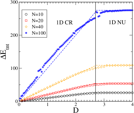
Figure 1: Energy barrier as a function of the anisotropy barrier $D$ for the $\alpha=d=1$. Different symbols indicate different number of spins in the linear array, as indicated in the legend. Dashed lines indicate the approximation Eq. (7). The vertical black line indicates $D=D_{cr}$, and separates the region of coherent rotation (CR, left), from the region of nucleation (NU, right).

Note that in case of nucleation ($DN>\Delta E_{\uparrow\downarrow}$), the effective energy barrier $\Delta E_{tnt}$ to be put in the Arrhenius Law should be increased by a term $D$, called single-spin flip. This extra term should be added only for continuous models, as the modified Heisenberg model we are considering, so that, $\tau_{0}\propto e^{D\beta}$ vindigni2 . This should be done since a single spin can continuously change from $S=1$ to $S=-1$ only passing the state $S=0$. While the two extreme states have the same magnetic anisotropy (since it is proportional to $DS^{2}$) the intermediate state $S=0$ has a barrier higher by a factor $D$. This additional spin-flip does not occur, for instance, in the Ising–like models, since there are no intermediate states between $S=1$ and $S=-1$.

In the following we analyzed the magnetic decay time in the canonical ensemble, using a modified Monte Carlo simulation metropolis ; nowak2 . As initial condition we choose all spins aligned along the easy axis, and from the exponential decay of the average magnetization, $\langle m(t)\rangle\propto e^{-t/\tau}$, we computed the magnetic decay time, $\tau$.

IV Enhanced Barrier

In this Section, we show our numerical results for the magnetization decay. They will clearly give evidence of the enhancement of the magnetization decay time due to long range interaction.

IV.1 One dimensional case

Here we focus on the one dimensional critical case.

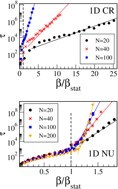
Figure 2: Magnetic decay times, $\tau$ vs the rescaled inverse temperature, $\beta/\beta_{stat}$ for $\alpha=d=1$ and different numbers of spins $N$ as indicated in the legend. Upper panel is characterized by coherent rotation with parameters $J=1$ and $D=0.05$ , while the lower by nucleation with $J=1/16$ and $D=0.5$. Different symbols refer to numerical results, while full lines in are the theoretical predictions $\exp(\beta\Delta E_{tnt})$. Specifically for coherent rotation, we have $\Delta E_{tnt}=DN$, while for nucleation, we have $\Delta E_{tnt}=\Delta E_{\uparrow\downarrow}+D$ (see text for explanations). Vertical dashed lines refer to the inverse rescaled statistical temperature $\beta=\beta_{stat}$ obtained by a standard mean field approach.

Our results for the magnetic decay time, are collected in Fig. 2, where we consider the case $\alpha=d=1$: magnetic decay times are shown in the upper panel for coherent rotation ($D\ll D_{cr}$) and in the lower panel for nucleation ($D\gg D_{cr}$). Samples with different number of particles experience different anisotropy energy barriers. As one can see the numerical results indicated by symbols well agree with the theoretical prediction given by Eq. (7), shown as full lines. Our results for coherent rotation, Fig. 2 (upper panel), clearly indicates that Brown’s theory of coherent rotation with an anisotropy energy barrier proportional to the particle volume ($V\propto N$ ) is still at work even for long range interacting systems. In Fig. 2 (lower panel), the case of nucleation is shown. Also in this case the anisotropy energy barrier is proportional to the particle volume. Let us remark that this behaviour is different for short range interacting systems, where in the one dimensional case, the anisotropic energy barrier is independent from the size of the system vindigni2 ; carbone . Note that for high temperature (small $\beta$ values) symbols with different number of spins lye upon the same curve, that turns out to be almost independent of $N$.

IV.2 Multidimensional case

Our results can be extended to higher dimensions. In particular we will show that for large enough particle, the anisotropic energy barrier is always proportional to the volume of the particle. Moreover we point out that for finite sized systems, the anisotropic energy barrier can grow even faster than the volume.

From Eqs (6) and (7), we have that while for coherent rotation, the anisotropy energy is always proportional to the volume of the particle, for nucleation the anisotropy energy can grow even faster than the volume of the particle, $\Delta E_{\uparrow\downarrow}\propto N^{2-\alpha/d}$. Since the anisotropy energy barrier is determined by the smallest of the two barriers, it follows that for sufficiently large particles the energy barrier will always be proportional to the particle volume since $V\propto N$. In particular, this means that even in the case of 3–d elongated particles, differently with what happens in the short range case, the energy barrier does not depend on the cross sectional area but on the whole particle volume.

This theoretical prediction has been numerically confirmed in Fig. 3, where we study the case of nucleation in thin parallelepipeds $L\times L\times\epsilon L$, in presence of a “ critical” interaction $\alpha=d=3$. We chose the aspect ratio $\epsilon=10$.

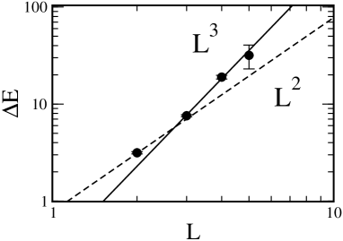
Figure 3: Energy barrier $\Delta E$ as a function of the side $L$ of the parallelepiped, obtained by an exponential fitting of the decay time vs the inverse temperature $\beta$. Here is $\alpha=3$, $J=1/20$ and $D=0.5$ (nucleation).

The energy barrier $\Delta E$ extracted from the numerical fit of the Arrhenius Law $\tau=\tau_{0}\exp(\beta\Delta E)$ has been plot as a function of the side $L$ of the parallelepiped. For sake of comparison the lines proportional to the cross section ($L^{2}$) and to the volume ($L^{3}$) has been drawn. As one can see without any doubt the barrier grows as the volume.

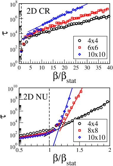
Figure 4: Decay time $\tau$ vs the rescaled inverse temperature $\beta/\beta_{stat}$ for a square lattice ($d=2$) with $\alpha=1$. for $J=1$ and $D=0.025$ (upper panel, coherent rotation); and for $J=1/40$ and $D=1/2$ (lower panel, nucleation). Symbols refer to numerical data, while full lines are the analytical prediction Eq. (7). Vertical dashed lines represent the rescaled inverse statistical temperature $\beta/\beta_{stat}=1$. Note that in case of coherent rotation (upper panel), the anisotropy energy is proportional to $DN$, while in the case of nucleation (lower panel), the anisotropy energy is proportional to $JN^{3/2}$. Lattice dimensions have been indicated in the legend

From Eqs (6) and (7), it also follows that, when $\alpha<d$ the anisotropy barrier can grow even faster than the volume of the particle. This can happen up to a critical value of the particle volume, for which $DN=\Delta E_{\uparrow\downarrow}$. Such an effect is a distinguished feature of long–range interaction and it is forbidden in the case of short range interactions. To confirme such theoretical prediction let us consider a square lattice ($d=2$) characterized by an exchange interaction decaying as $1/r$ ($\alpha=1$). Even in this case we can distinguish between the regime of coherent rotation (large anisotropy barriers $D$) from that of nucleation (small $D$ values). The results of our simulation have been shown in Fig. 4. In the lower panel the theoretical predictions have been indicated as full lines while symbols represents numerical results from Montecarlo simulation. As one can see the agreement with the theory, which predicts an energy barrier $\Delta E_{tnt}\propto JN^{3/2}$ is fairly good. For sake of comparison, the regime of coherent rotation (Fig. 4, upper panel) is also shown, indicating that, in this case, the energy barrier is proportional to the volume of the particle, namely $\Delta E_{tnt}\propto DN$.

Another important point to be discussed is in which temperature range the Arrhenius Law with the exponent given by Eq. (7) holds. In the cases of coherent rotation and nucleation, see also Ref. brown , we might expect that the Arrhenius Law is valid only when $k_{B}T\ll\Delta E_{tnt}$. Clearly this gives an upper bound for the temperature for which Eq. (4) is valid. Moreover it should be $T\ll T_{stat}$, where the latter is the temperature at which the barrier at $m=0$ in the free energy vanishes (and it coincides with the temperature at which a phase transition occurs in the thermodynamic limit). It is very interesting that, computing $T_{stat}=1/k_{B}\beta_{stat}$ by means of a standard mean field approach, one gets a very nice estimate of the validity range of the Arrhenius Law (see dashed vertical lines in Figs. 2 and 4). Nevertheless we stress that this delicate point needs further analysis to be clarified.

V Coherent Rotation and Nucleation

Let us notice that the use of the words coherent rotation and nucleation, are not only ways to label two different mechanisms taken from the short range models, but correspond to the spin dynamics. To prove that we first consider in Fig. 5 two different situations taken from the upper (coherent rotation) and the lower panel (nucleation) of Fig. 4. In particular we consider one single Montecarlo trajectory and we plot, in Fig. 5 the value of $M=|\frac{1}{N}\sum_{i=1}^{N}\vec{S}_{i}|$ and $m=\frac{1}{N}\sum_{i=1}^{N}S^{z}_{i}$, as a function of the Metropolis time. It is clear that while in the case of coherent rotation (upper panel of Fig. 5) $M\approx 1$ and $m$ change its sign, for nucleation (lower panel of Fig. 5) one has $M\simeq|m|$.

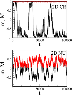
Figure 5: Upper panel (coherent rotation) for a square lattice $6\times 6$, $\beta=5$. Lower panel (nucleation) for a square lattice $8\times 8$ and $\beta=4.5$. In both panels the red curve refers to $M$, while the black one to $m$.

As an interesting consequences of the coherent motion of the spins during the magnetic reversal, we show here, focusing on the one dimensional case, that one can estimate the whole probability distribution of the magnetization in the canonical ensemble, $P_{T}(m)$ at low temperature and around $m=0$.

Note that the knowledge of the probability distribution of the magnetization allows one to compute the magnetic decay time:

$$\tau\propto e^{\beta\Delta F}=\frac{P_{T}(m_{max})}{P_{T}(m_{min})},$$ (8)

where $P_{T}(m_{max,min})$ stands for the maximum/minimum value of the probability distribution.

Due to the coherent motion of all spins it is possible to express the energy of the system as a function of the total magnetization along the easy axis; from the knowledge of $E(m)$ we can compute $P_{T}(m)$ since:

$$P_{T}(m)\ dm=P_{T}(E)\ dE=e^{-E(m)/k_{B}T}\rho(E)\ dE$$

where $\rho(E)$ is the density of states at fixed energy. Using the fact that $\rho(E)dE=\rho(m)dm$, where $\rho(m)$ is the density of states at fixed magnetization, we have:

$$P_{T}(m)\ dm=e^{-E(m)/k_{B}T}\ \rho(m)\ dm.$$ (9)

Let us compute $E(m)$ for coherent rotation and nucleation. When the decay of the magnetization occurs through coherent rotation we have $\vec{S}_{i}\vec{S}_{j}=1$, and $S_{i}^{z}=\langle S^{z}\rangle=m$ so that, from Eq. (5) we have:

$$E(m)=-J/2\sum 1/r_{i,j}^{\alpha}-DNm^{2}.$$ (10)

Since all spins move coherently on a sphere, the density of states at fixed magnetization along any axis is constant, $\rho(m)=const.$ Moreover the first term in the r.h.s. of Eq. (10) is independent of $m$ and we have (for coherent rotations):

$$P_{T}(m)\propto e^{\beta DNm^{2}}.$$ (11)

We verified numerically that Eq. (11) gives an excellent approximation of the probability distribution of the magnetization around $m=0$ in the coherent rotation regime, see Fig. 6 (upper panel).

In case of nucleation the possible configurations which the system can visit can be obtained assuming that magnetic decay occurs by first reversing one of the edge spins, then its nearest neighbor, and then the spin immediately after until all spins are reversed. If we have $k$ spins on the left pointing upwards and $N-k$ spins pointing downwards, we can write the energy of this configuration as

$$E(k,N)=E_{min}(k)+E_{min}(N-k)+W(k,N-k),$$ (12)

where $W(k,N-k)$ is the interaction energy between the two neighbors blocks of $k$ and $N-k$ spins and

$$E_{min}(k)=-J/2\sum^{k}_{i=1}\sum^{k}_{j\neq i}1/r_{i,j}^{\alpha}-Dk,$$ (13)

is the minimal energy for a system of $k$ spins. The minimal energy of a system of $N$ spins can be easily obtained from (12) by changing the sign of $W(k,N-k)$,

$$E_{min}(N)=E_{min}(k)+E_{min}(N-k)-W(k,N-k).$$ (14)

Taking into account that $m=(2k-N)/N$ is the magnetization of a system composed by $k$ spins along the easy axis and $N-k$ opposite to it, one gets,

$$E(m)=2E_{min}(N_{+})+2E_{min}(N_{-})-E_{min}(N),$$ (15)

where $N_{\pm}=N(1-m)/2$. In this case it is more difficult to estimate $\rho(m)$. Assuming, also in this case $\rho(m)=const.$, from the knowledge of $E(m)$ (Eq. (15)), we obtain $P_{T}(m)\propto e^{-\beta E(m)}$ which agrees very well (apart close to $m=\pm 1$) with numerical results in the nucleation regime, see Fig. 6 (lower panel).

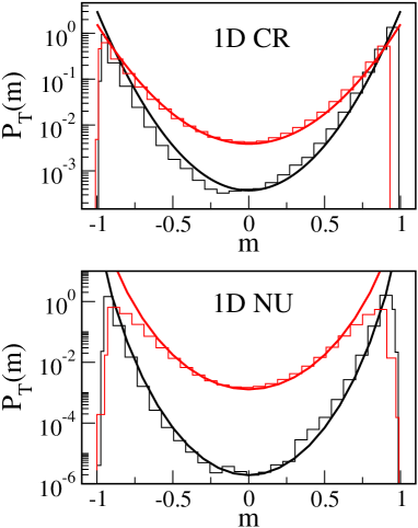
Figure 6: Probability distribution of the magnetization $P_{T}(m)$ vs the magnetization $m$ for $\alpha=d=1$, $N=20$ and different temperatures $\beta=1/k_{B}T$. Upper panel is for $J=1$ and $D=0.05$ (coherent rotation regime) and $\beta=6$ (upper red hystogram), $\beta=9$ (lower black hystogram). The lower panel is for $J=1/16$ and $D=0.5$ (nucleation) and $\beta=8$ (upper red hystogram), $\beta=11$ (lower black hystogram). Hystograms represent numerical data, while smooth curves analytical results.

The validity of Eq. (4) and of our method to approximate $P_{T}(m)$ at low temperature, have been tested for a wide range of values of $\alpha$ (even for short range interactions) and a detailed study will be reported elsewhere fausto .

VI Conclusions

In conclusion we propose a general method to determine the anisotropic energy barrier in spin systems. The barrier, which determines magnetic decay times, can be computed from the topological non-connectivity energy threshold in the corresponding isolated systems. Our analysis shows that for long range interaction two different regimes can be identifyied, coherent rotation and nucleation. In the first regime we have predicted and numerically confirmed that magnetic decay time depends exponentially on the volume of the particle. Nevertheless, in the regime of nucleation, the magnetic barrier depends on a suitable power of the volume, $V^{2-\alpha/d}$, where $\alpha<d$ is the range of interaction and $d$ is the lattice dimension. These facts have two remarkable consequences. The first one is that magnetic decay times depend exponentially on the volume of the particle and not on its cross sectional area, as happens for short range interactions. The second one is that, the fast growth of the magnetic barrier with the volume, gives rise to the possibility to observe long-lived metastable ferromagnetism in finite systems at high temperature which is ruled out for short range interaction.

We acknowledge useful discussion with B. Goncalves, D. Mukamel, S. Ruffo, R. Trasarti-Battistoni and A. Vindigni. This work has been supported by Regione Lombardia and CILEA Consortium through a Laboratory for Interdisciplinary Advanced Simulation (LISA) Initiative (2010) grant [link:http://lisa.cilea.it] ”. Support by the grant D.2.2 2010 (Calcolo ad alte prestazioni) from Universitá Cattolica is also acknowledged.

References

- (1) W. Wernsdorfer et al., Phys. Rev. Lett. 77, 1873 (1996); Phys. Rev. Lett. 78, 1791 (1997); Phys. Rev. Lett. 79, 4014 (1997).
- (2) C. Coulon, H. Miyasaka, R. Clerac, Structure and Bonding, 2006, Volume 122/2006, 163-206.
- (3) A. Vindigni, Inorganica Chimica Acta 361, 3731 (2008).
- (4) D. Hinzke and U. Nowak, Phys. Rev. B 61, 6734 (2000).
- (5) P.Gambardella et al., Nature 146, 301 (2002).
- (6) A.B. Shick, F. Máca, P.M. Oppeneer, JMMM 290-291, 257 (2005); A. Vindigni, A. Rettori, M.G. Pini, C. Carbone, P. Gambardella, Appl. Phys. A 82, 385 (2006); Y. Li, Bang-Gui Liu, Phys. Rev. B 73, 174418 (2006); L. He, D. Kong, C. Chen, J. Phys. C 19, 446207 (2007).
- (7) N.D. Mermin, H. Wagner, Phys. Rev. Lett. 17, 1133 (1966) ; P.Bruno, Phys. Rev. Lett. 87, 137203 (2001).
- (8) T. Dauxois, S. Ruffo, E. Arimondo, M. Wilkens Eds., Lect. Notes in Phys., 602, Springer (2002).
- (9) A.H. Macdonald, P. Schiffer and N. Samarth, Nature Materials 4, 195 (2005).
- (10) J.M. Coey, M. Venkatesan and C.B. Fitzgerald, Nature Materials 4, 173 (2005).
- (11) L. Neél, Ann. Geophys., 5, 99 (1949).
- (12) W.F. Brown, Phys. Rev. 130, 1677 (1963).
- (13) H.B. Braun, Phys. Rev. B 50,16501 (1994); H.-B. Braun, J. Appl. Phys. 76, 10 (1994); H.-B. Braun, J. Appl. Phys. 75, 9 (1994); H.B. Braun, Jour. Appl. Phys. 99, 08F908 (2006);
- (14) U. Nowak et al., Phys. Rev. B 72, 172410 (2005).
- (15) D. Hinzke and U. Nowak, Phys. Rev. B 58, 265 (1998); U. Nowak and D. Hinzke, Journal of Applied Physics 85, 4337 (1999).
- (16) M. Bode, O. Pietzsch, A.Kubetzka, and R. Wiesendanger, Phys. Rev. Lett. 92, 067201 (2004).
- (17) R.B. Griffiths, C.-Y. Weng and J.S. Langer, Phys. Rev. 149, 301 (1966).
- (18) F. Borgonovi, G. L. Celardo, M. Maianti, E. Pedersoli, J. Stat. Phys. 116, 516 (2004); G. Celardo, J. Barré, F.Borgonovi, and S.Ruffo, Phys. Rev. E 73, 011108 (2006); R. Trasarti-Battistoni, F. Borgonovi, and G. L. Celardo, EPJ B 50, 69 (2006); F. Borgonovi, G. L. Celardo, and R. Trasarti-Battistoni, EPJ B 50, 27 (2006).
- (19) D. Mukamel, S. Ruffo, and N. Schreiber, Phys. Rev. Lett. 95, 240604 (2005); Freddy Bouchet, Thierry Dauxois, David Mukamel, and Stefano Ruffo, Phys. Rev. E 77, 011125 (2008); A. Campa, R. Khomeriki, D. Mukamel, and S. Ruffo, Phys. Rev. B 76, 064415 (2007), A. Campa, T. Dauxois, S. Ruffo Phys. Rep 480, 57 (2009).
- (20) F. Borgonovi, G. L. Celardo, A. Musesti, R. Trasarti-Battistoni, and P. Vachal, Phys. Rev. E 73, 026116 (2006).
- (21) F. Borgonovi, G. L. Celardo, B. Goncalves and L. Spadafora, Phys. Rev. E, 77, 061119 (2008).
- (22) N. Metropolis, A. W. Rosenbluth, M. N. Rosenbluth, A. H. Teller and E. Teller. J. Chem. Phys. 21, 1087, (1953).
- (23) M.J. Calderon and S. Das Sarma, Annals of Physics 322, 2618 (2007).
- (24) P.J. Priour, Jr. E. H. Hwang and S. Das Sarma, Phys. Rev. Lett. 92, 117201 (2004).
- (25) F. Borgonovi and G.L. Celardo, in preparation.