Dynamic modeling of gene expression in prokaryotes: application to glucose-lactose diauxie in Escherichia coli

Abstract

Coexpression of genes or, more generally, similarity in the expression profiles poses an unsurmountable obstacle to inferring the gene regulatory network (GRN) based solely on data from DNA microarray time series. Clustering of genes with similar expression profiles allows for a course-grained view of the GRN and a probabilistic determination of the connectivity among the clusters. We present a model for the temporal evolution of a gene cluster network which takes into account interactions of gene products with genes and, through a non-constant degradation rate, with other gene products. The number of model parameters is reduced by using polynomial functions to interpolate temporal data points. In this manner, the task of parameter estimation is reduced to a system of linear algebraic equations, thus making the computation time shorter by orders of magnitude. To eliminate irrelevant networks, we test each GRN for stability with respect to parameter variations, and impose restrictions on its behavior near the steady state. We apply our model and methods to DNA microarray time series’ data collected on Escherichia coli during glucose-lactose diauxie and infer the most probable cluster network for different phases of the experiment.

Keywords: Gene regulatory networks, DNA microarray, gene product degradation, gene clustering, optimization, dynamic robustness

1 Introduction

The information encoded in the genome of living organisms has presented a new level of complexity that continues to challenge the mind. Both theoretical and experimental studies have proven to be very difficult mainly due to the large dimension of the system of interacting genes. Even the simplest of prokaryotic cells contain some 4000 genes of which a significant fraction participates directly or indirectly in regulating (enhancing or inhibiting) the expression of one another. Despite these daunting obstacles, progress in unraveling Gene Regulatory Networks (GRN) has been made mainly due to new experimental methods that allow for more detailed studies of the intricate mechanisms within the living cells.

In particular, owing to the development of DNA microarrays techniques, it has become possible to probe the behavior of thousands of genes simultaneously over a certain course of time. The advantage of recording the temporal evolution of the genome (or at least a large part of it) as compared to having the same information on only a handful of genes is obviously quite important and has led to the onset of new types of studies, e. g. see [1] and [2]. The challenge of inferring the GRN however still persists due to the abovementioned problem of large dimensionality, but also because of (still) partial and noisy data. This makes improvements in both theory and experiment equally important.

The difficulty of dealing with a large number of genes has forced one to proceed to various simplifications of the GRN problem. In many studies researchers have made use of simple models for the gene-gene product (GP) interactions including Boolean and Baysian networks [3], and linear coupled differential equations as in the works by [4], [5] and [6]. Although simple models are attractive, especially when dealing with a large number of genes, they often suffer from lack of physical relevance. The biochemical interactions on the molecular level are known to be more complicated than most simple models can account for. Nevertheless, the correlations between genes that many simple models predict can provide a course-grained view of the GRN. Another popular trend in simplifying the GRN problem is to focus on a subset of genes that are known to regulate each other under the assumption that no other gene has a regulatory influence on this sub-network. This type of approximation makes more complicated models, i.e. non-linear models, feasible as was shown in [7] and [8].

An additional difficulty is related to the fact that many genes are coexpressed and exhibit thus basically the same expression profiles, and that even non-coexpressed genes may have similar profiles under certain circumstances and/or during a certain time span. As a consequence one cannot obtain the information about the correlations among all genes from DNA microarray data alone, regardless of the quality or complexity of the model at hand. This issue can be partly resolved by grouping genes with similar expression profiles into clusters, which allows one to shift focus from individual genes to the study of how clusters influence each other. Consequently, the dimension of the problem is reduced to the number of clusters, which in many cases is much less than a hundred. Such a drastic reduction in dimensionality also opens the door to more complicated (and hence more accurate) models, and can reveal a more realistic course-grained picture of the GRN. The last difficulty we address here is the multitude of possible GRNs that generate the same gene (or cluster) expression profile. This is sometimes referred to as gene elasticity [9].

In this paper we attempt to further the methods of identifying the connections among gene clusters on the basis of DNA microarray time series and propose criteria that eliminate many possible solutions for the gene cluster network. The system under consideration consists of E. coli bacteria in a glucose-lactose environment. The GRN model we design takes into account gene-GP and GP-GP interactions that are derived from physical arguments. Our work is a further step towards reliably predicting cluster gene networks on the basis of DNA microarray time series.

The paper is structured as follows. In section one we give a brief description of the known regulatory mechanisms in prokaryotic cells and derive a physical model that describes them. We then adapt this model to be suited for cluster-cluster interactions. In section two we discuss the procedure of parameter identification and parameter reduction. The application of our model to E. coli during glucose-lactose diauxie is covered in section three where we also discuss the criteria for GRN selection. In the last section, we summarize our results and discuss possible issues as well as outlooks for further studies in this field.

2 Modeling the biochemical processes

The living cell is like a small factory whose products (GPs), i.e. RNA and proteins, sustain it, allow it to divide, and even terminate its life. The cell absorbs various chemicals from the environment and uses them for many purposes. Some of them serve as fuel to drive its internal machinery, others are used for intra-cell or cell-to-cell signal propagation and many other essential functions. Genes and their promoter sequences act as pieces of software that hold the instructions for synthesizing RNA molecules, some of which, i.e. the (messenger) mRNAs, are then translated into proteins; all RNAs and proteins are collectively referred to as GPs and we will make no distinction between them in what follows.

The GPs that bind to regulatory promoter sites and hence regulate the transcription of genes (direct regulation) are called transcription factors (TF). Other GPs which are not TFs themselves but bind to TFs can also influence gene regulation (indirect regulation). In fact, virtually all GPs can play a role, either directly or indirectly, in the regulation of gene expression. Depending on the external environment some genes may be highly active (expressed) while others can have low output or even be completely off. Which gene is expressed and when depends on the abundance of specific GPs and their affinity to bind the gene’s regulatory sites or other GPs. Since gene regulation is much more complicated in eukaryotes than in prokaryotes (see e.g. [10]) we concentrate on the latter. Hence, the rest of this article deals exclusively with prokaryotes.

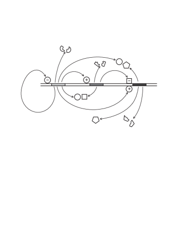
Figure 1: A GRN of three genes showing the regulatory pathways. The circle, square, and pentagon represent the GPs synthesized by genes 1, 2, and 3, respectively (from left to right), and the broken circle, square, and pentagon represent degraded GPs. The $+$ and $-$ signs correspond to activation and repression respectively. The third gene synthesizes a GP that is not a TF as it does not directly regulate any of the other two genes. Also shown is the interaction among the different GPs.

2.1 A model of prokaryotic gene regulation

In figure 1. we show a toy model of three genes that mutually interact through their GPs. The arrows indicate the gene-GP and GP-GP interaction pathways. Because of thermodynamic instabilities, degradation by enzymes, transport to other cell compartments, and effects of dilution upon cell growth, GPs inevitably degrade or loose activity in some characteristic time. Depending on this time GPs can have either long or short lasting influence on genes. In what follows we present a mathematical description of how the GPs influence a gene’s transcription rate.

We begin by assuming that time delays between the production of GPs and their influence on a gene are negligible compared to the times over which the concentration levels change significantly. This assumption is supported by comparing the typical diffusion and transcription rates, and amounts to neglecting the effects of translational regulation and any distinction between RNA and proteins.

The most general set of differential equations describing a system of $M$ genes under constant environment has the form

$$\dot{X}_{i}=R_{i}({\bf X},{\bf C}_{i})$$ (1)

where $i=1,...,M$. $R_{i}({\bf X},{\bf C}_{i})$, ${\bf X}=(X_{1},...,X_{M})$ and ${\bf C}_{i}=(C^{1}_{i},...,C^{N}_{i})$ are an influence function, the concentration vector of GPs and the set of all parameters pertaining to gene $i$, respectively. The influence function consists of two terms:

$$R_{i}({\bf X},{\bf C}_{i})=f_{i}({\bf X},{\bf C}_{i})+g_{i}({\bf X},{\bf C}_{i}),$$ (2)

with

$$f_{i}({\bf X},{\bf C}_{i})>0,\,\,\,\,\,\,\,\,g_{i}({\bf X},{\bf C}_{i})<0.$$ (3)

The first term in Eq. (2) depends on the abilities of various GPs to bind a promoter of gene $i$, i. e. the binding affinities, and on the efficiency of recruiting the RNA-polymerase, while the second term gives the rate of GP degradation. To understand the structure of $f_{i}$, let us first look at a simple example of two TF’s competing for the same promoter. Suppose that the transcription of gene $i$ is enhanced by two activators $1$ and $2$. The probability that say $1$ will bind to the promoter is (see [11])

$$P_{A}^{1}({\bf X},{\bf A}_{i})=\frac{A_{i1}X_{1}}{1+A_{i1}X_{1}+A_{i2}X_{2}},$$ (4)

with $X_{1}$ and $X_{2}$ being the concentrations of GP $1$ and $2$. The index $A$ stands for activation. The parameters $A_{i1}$ and $A_{i2}$ are proportional to the frequencies of collisions between the gene’s promoter and the GPs $1$ and $2$, and to their binding affinities. The term 1 in the denominator indicates that the promoter may be unoccupied, and the term $A_{i2}X_{2}$ comes from the fact that the GPs $1$ and $2$ compete for the same promoter. Indeed, if the concentration of GP $2$ becomes very large, the probability for GP $1$ to bind the promoter becomes low. On the other hand, if the converse were to occur this probability would approach one.

For a transcription to occur the part of the promoter which admits only activators must be occupied while the part that admits repressors must be unoccupied. The probability for such a scenario is given by the probability that an activator is bound to the promoter multiplied by the probability that the converse is true for a repressor. The probability for gene $i$ to have a certain rate of transcription is then

$$P_{i}({\bf X},{\bf\Gamma}_{i})=P_{A}({\bf X},{\bf A}_{i})(1-P_{S}({\bf X},{\bf S}_{i})),$$ (5)

where ${\bf\Gamma}_{i}=({\bf A}_{i},{\bf S}_{i})$, $A^{j}_{i}\geq 0$, $S^{j}_{i}\geq 0$,

$$P_{A}({\bf X},{\bf A}_{i})=\frac{A^{j}_{i}X_{j}}{1+A^{j}_{i}X_{j}}$$ (6)

and

$$P_{S}({\bf X},{\bf S}_{i})=\frac{S^{j}_{i}X_{j}}{1+S^{j}_{i}X_{j}}.$$ (7)

The repeated index $j$ sums over all the GPs which influence gene $i$: $A^{j}_{i}X_{j}=\sum_{j}A_{ij}X_{j}$. The total probability for gene $i$ to be occupied by any activator is then

$$P_{i}({\bf X},{\bf\Gamma}_{i})=\frac{A^{j}_{i}X_{j}}{(1+A^{j}_{i}X_{j})(1+S^{j}_{i}X_{j})}.$$ (8)

Note that in deriving this equation we made the assumption that the expression of a gene may be activated or repressed by a single GP, and does not require complexes of GPs or cascades of interacting GPs. The motivation for this choice is that most genes in prokaryotes are regulated by forming DNA-protein complexes involving single proteins.

Since ${\bf X}$ is a stochastic variable we have to average the transcription rate over an ensemble of many cells under the same external conditions:

$$f_{i}({\bf X},{\bf\Gamma}_{i})=\langle r_{i}P_{i}({\bf X},{\bf\Gamma}_{i})\rangle.$$ (9)

The parameter $r_{i}$ is the maximum transcription rate corresponding to the saturation point at $A^{j}_{i}X_{j}\rightarrow\infty$ and is taken to be independent of the particular combination of GPs that bind to gene $i$. Note that by averaging over an ensemble, the stochastic variables of the system become determininstic. For that purpose we first write in Eq. (9) $X_{i}=x_{i}+\eta_{i}$ where $x_{i}$ is the average expression of gene $i$ over an ensemble of identical cells and $\eta_{i}$ is a Gaussian noise function of the same gene. We then expand with respect to $\eta$:

$$f_{i}({\bf X},{\bf\Gamma}_{i})=r_{i}\left[P_{i}({\bf x},{\bf\Gamma}_{i})+\frac{\partial}{\partial x_{j}}P_{i}({\bf x},{\bf\Gamma}_{i})\langle\eta_{j}\rangle+O(\langle\eta^{2}\rangle)+...\right].$$ (10)

Since $\langle\eta_{j}\rangle=0$ for a Gaussian function, the first order approximation of the rate function $f_{i}$ in Eq. (10) yields

$$f_{i}({\bf X},{\bf\Gamma}_{i})=r_{i}P_{i}({\bf x},{\bf\Gamma}_{i})=r_{i}\frac{A^{j}_{i}x_{j}}{(1+A^{j}_{i}x_{j})(1+S^{j}_{i}x_{j})}.$$ (11)

Various environmental conditions within the cell can cause the GPs to degrade, or loose their activity, after some characteristic time $\tau_{c}$ [12]. Since the ability of a GP to influence a gene depends on how long it remains active, those GPs with a long $\tau_{c}$ are more likely to bind a gene’s promoter. The converse is true for GPs with short $\tau_{c}$. We hypothesize that GPs mutually interact to either prolong (e.g. through stabilizing complexes) or shorten (e.g. through degradation by proteases) their $\tau_{c}$ in order to provide another channel for gene control. The nature of GP-GP interaction is too complicated for our purposes here and will not be treated on the molecular level. Instead we want to write down a course-grained expression that corresponds to the behavior expected from the arguments just outlined. In particular, we expect that overabundance of any one GP would saturate its influence on other GPs. On the basis of this assumption, we define a general $\bf X$-dependent degradation rate $k_{i}$ of the form:

$$\frac{1}{\tau_{i}}\equiv k_{i}({\bf X},{\bf\ell}_{i})=\frac{K_{i}^{+}+K_{i}^{-}e^{K_{i}^{j}X_{j}}}{1+e^{K_{i}^{j}X_{j}}},$$ (12)

where ${\bf\ell}_{i}=(K_{i}^{+},K_{i}^{-},{\bf K}_{i})$, $K^{\pm}_{i}\geq 0$, $-\infty<K^{j}_{i}<\infty$, and $\tau_{i}$ is the characteristic time associated with GP i. The two parameters $K_{i}^{+}$ and $K_{i}^{-}$ symbolize the maximum and minimum degradation rate respectively. The matrix elements $K_{i}^{j}$ give the influence of GP $j$ on GP $i$. Notice that when $K_{i}^{j}X_{j}$ is large and positive, $k_{i}({\bf X},{\bf\ell}_{i})$ approaches $K_{i}^{-}$ which corresponds to the longest $\tau_{i}$ for GP $i$ while the opposite limit yields $K_{i}^{+}$ - the shortest $\tau_{i}$. The sign of each matrix element $K_{i}^{j}$ determines whether GP $j$ has a stabilizing (a plus sign) or destabilizing (a minus sign) influence on GP $i$. As before, Eq. (12) must be averaged over the ensemble of cells. The degradation term $g_{i}$ of Eq. (2) can now be written as

$$g_{i}({\bf X},{\bf\ell}_{i})=-k_{i}({\bf X},{\bf\ell}_{i})X_{i}.$$ (13)

Making the same substitution as before, $X_{i}=x_{i}+\eta_{i}$, and expanding to the second order on $\eta$ leads, after ensemble averaging, to the following first order approximation:

$$g_{i}({\bf x},{\bf\ell}_{i})=-\frac{K_{i}^{+}+K_{i}^{-}e^{K_{i}^{j}x_{j}}}{1+e^{K_{i}^{j}x_{j}}}x_{i}$$ (14)

Combining Eqs. (11) and (14), the influence function in Eq. (1) becomes

$$R_{i}({\bf x},{\bf\Gamma}_{i},{\bf\ell}_{i}) = f_{i}({\bf x},{\bf\Gamma}_{i})-k_{i}({\bf x},{\bf\ell}_{i})x_{i}$$ (15)

$$= r_{i}\frac{A^{j}_{i}x_{j}}{(1+A^{j}_{i}x_{j})(1+S^{j}_{i}x_{j})}-\frac{K_{i}^{+}+K_{i}^{-}e^{K_{i}^{j}x_{j}}}{1+e^{K_{i}^{j}x_{j}}}x_{i}.$$

2.2 A model of gene cluster regulation

Given that genes with similar expression profiles cannot be differentiated on the basis of data from microarray time series, we are led to group genes into clusters according to the similarity of their profiles. This compels us to rewrite our model in terms of gene clusters and treat the deviations in concentration levels from the cluster average as external perturbations. Let us write $x_{i}=\bar{X}_{q}+\xi_{i}$, where $\xi_{i}$ is the deviation of gene $i$ from the average concentration $\bar{X}_{q}$ of cluster $q$. This transforms all terms of the form $A_{i}^{j}x_{j}$ into $A_{i}^{p}\bar{X}_{p}+A_{i}^{j}\xi_{j}$, where $A_{i}^{p}=\sum_{j}A_{i}^{j}$ is the sum over all genes in cluster $p$ denoted $N_{p}$, and the sum over $p$ goes over all clusters $N_{c}$. Inserting this into Eq. (1), expanding the right hand side up to first order on $\xi$, and averaging over cluster $q$ and over the ensemble of cells yields

$$\dot{\bar{X}}_{q} = \varphi_{q}({\bf\bar{X}})+\delta_{q},$$ (16)

$$\varphi_{q}({\bf\bar{X}}) = F_{q}({\bf\bar{X}})-K_{q}({\bf\bar{X}})\bar{X}_{q},$$ (17)

where ${\bf\bar{X}}=(\bar{X}_{1},...\bar{X}_{N_{c}})$,

$$F_{q}({\bf\bar{X}})=\frac{1}{N_{q}}\sum_{i=1}^{N_{q}}f_{i}({\bf\bar{X}},{\bf\Gamma}_{i}),$$ (18)

$$K_{q}({\bf\bar{X}})=\frac{1}{N_{q}}\sum_{i=1}^{N_{q}}k_{i}({\bf\bar{X}},{\bf\ell}_{i}),$$ (19)

and

$$\delta_{q}=\frac{1}{N_{q}}\sum_{i=1}^{N_{q}}\bigg{[}\sum_{j=1}^{N_{q}}\left(\frac{\partial f_{i}}{\partial\xi_{j}}-X_{i}\frac{\partial k_{i}}{\partial\xi_{j}}\right)\langle\xi_{j}\rangle-k_{i}\langle\xi_{i}\rangle-\langle\dot{\xi}_{i}\rangle\bigg{]}.$$ (20)

In what follows, we only consider the zeroth order approximation: $\delta_{q}=0$.

To complete our journey from genes to clusters we must reformulate the functions under the summation in Eqs. (18), (19). The concentration levels $\bar{X}_{p}$ already represent the cluster average, but the parameters $r_{q}$, $A_{i}^{p}$, $S_{i}^{p}$, $K_{i}^{+}$, $K_{i}^{-}$, and $K_{i}^{p}$ need to be replaced with some effective parameters $\rho_{q}$, $\alpha_{q}^{p}$, $\beta_{q}^{p}$, $\kappa_{q}^{+}$, $\kappa_{q}^{-}$, and $\kappa_{q}^{p}$, respectively. Even though doing this alters the local behavior of the multivariable functions defined in Eqs. (18) and (19), their general behavior will remain the same given an appropriate set of effective parameters. In other words, if one takes several functions that follow a certain behavior, i.e. starting linearly near zero and saturating for large values, their average will produce a function with the same behavior. A downside to this reformulation is a loss of oversight of the connection between the original set of parameters $(r_{q},A_{q}^{p},S_{q}^{p},K_{q}^{+},K_{q}^{-},K_{q}^{p})$ and the effective set ${\bf a}\equiv(\rho_{q},\alpha_{q}^{p},\beta_{q}^{p},\kappa_{q}^{+},\kappa_{q}^{-},\kappa_{q}^{p})$. The above reasoning thus yields the following model:

$$F_{q}({\bf\bar{X}})=\rho_{q}\frac{\alpha_{q}^{p}\bar{X}_{p}}{(1+\alpha_{q}^{p}\bar{X}_{p})(1+\beta_{q}^{p}\bar{X}_{p})}$$ (21)

$$K_{q}({\bf\bar{X}})=\frac{\kappa_{q}^{+}+\kappa_{q}^{-}e^{\kappa_{q}^{p}\bar{X}_{p}}}{1+e^{\kappa_{q}^{p}\bar{X}_{p}}}$$ (22)

This model contains a large number of parameters compared to the number of data points, which raises the issue of overfitting. In the following sections we address this problem and demonstrate how a lower bound on the total number of parameters necessary to fit the data can be determined through parameter reduction.

3 Parameter identification

Having formulated a dynamical model of the cluster network we move on to identifying the unknown parameters ${\bf a}$. A standard practice is to define a distance function

$$d({\bf a})=\frac{1}{\sqrt{N_{t}N_{c}}}\left[\sum_{q=1}^{N_{c}}\sum_{t=1}^{N_{t}}\left[\frac{d}{dt}\bar{X}_{q}(t)-\varphi_{q}({\bf\bar{X}},{\bf a})\right]^{2}\right]^{1/2},$$ (23)

where $N_{t}$ is the number of time points provided by the data, and $N_{c}$ represents the number of clusters. In order to estimate the derivatives $d{\bar{X}}_{q}(t)/dt$ one must choose an interpolating function fitting the data points (discussed further in the next section). The function $\varphi_{q}({\bf\bar{X}},{\bf a})$ defines the model; it is given by eq. (17). Minimizing $d({\bf a})$ with respect to all the parameter sets ${\bf a}$ gives the model that fits the data the best.

The minimization problem depends heavily on the total number of parameters to be optimized and so, reducing the number of parameters is a valuable endeavor. We can start by noticing that if the parameter sets ${\bf a}_{q}$ for each cluster $q$ are independent of each other one can minimize the parameter function

$$d_{q}({\bf a}_{q})=\frac{1}{\sqrt{N_{t}}}\left[\sum_{t=1}^{N_{t}}\left[\frac{d}{dt}{\bar{X}}_{q}(t)-\varphi_{q}({\bf{X}},{\bf a}_{q})\right]^{2}\right]^{1/2},$$ (24)

with respect to the parameters ${\bf a}_{q}$ for each cluster separately. In this manner, the problem is reduced from optimizing $3N_{c}(N_{c}+1)$ parameters in one step to optimizing $3(N_{c}+1)$ parameters $N_{c}$ times.

3.1 Parameter reduction

We now present a useful method for reducing the number of parameters of specific types of models, namely those of the form $\varphi_{q}({\bf\bar{X}},\omega_{q}^{p}\bar{X}_{p},{\bf\nu}_{q})$, where at least some of the parameters, i. e. $\omega_{q}^{p}$s, range from $-\infty$ to $+\infty$. The remaining parameters, ${\bf\nu}_{q}$, are positive.

The temporal profile of each cluster consists of discrete time points. In order to determine the functions $d{\bar{X}}_{q}/dt$ one must interpolate the data points with a smooth continuous curve. We chose for that purpose polynomial functions of order $w$:

$$\bar{X}_{q}=\sum_{n=0}^{w}c_{qn}t^{n}.$$ (25)

Inserting Eq. (25) into $\varphi_{q}({\bf\bar{X}},\omega_{q}^{p}\bar{X}_{p},{\bf\nu}_{q})$ gives

$$\varphi_{q}({\bf\bar{X}},\omega_{q}^{p}\bar{X}_{p},{\bf\nu}_{q})=\varphi_{q}(c_{qn}t^{n},\omega_{q}^{p}c_{pn}t^{n},{\bf\nu}_{q})$$ (26)

where we again sum over repeated indices. We can now define the new matrix element $B_{qn}=\omega_{q}^{p}c_{pn}$ which allows us to rewrite Eq. (24) as

$$d_{q}(\textbf{B}_{q},{\bf\nu}_{q})=$$

$$\frac{1}{\sqrt{N_{t}}}\left[\sum_{t=1}^{N_{t}}\left[c_{qn}nt^{n-1}-\varphi_{q}(c_{qn}t^{n},B_{qn}t^{n},{\bf\nu}_{q})\right]^{2}\right]^{1/2}.$$ (27)

The number of parameters to be determined for each cluster now equals $w+1$ plus the number of elements in the set ${\bf\nu}_{q}$. This simple procedure reduces the number of parameters and provides a degree of control when interpolating the data points. For instance, one may want to use low order polynomials at the expense of good data fit in order to reduce the number of parameters and thus avoid the problem of overfitting.

After determining the new parameters $B_{qn}$ by minimizing Eq. (3.1) we can solve for the original matrix elements $\omega_{q}^{p}$. Notice however, that if $w$ is less than the dimension of matrix $\omega_{q}^{p}$ we end up with many different solutions for the parameter set $(\omega_{q}^{i_{0}},...,\omega_{q}^{i_{w}})$ depending on what integers we assign to the indices $i_{0}...i_{w}$. For instance, if $w=4$ then we may solve for the parameter sets ($\omega_{q}^{1},\omega_{q}^{3},\omega_{q}^{7},\omega_{q}^{8},\omega_{q}^{9})$ or $(\omega_{q}^{2},\omega_{q}^{5},\omega_{q}^{6},\omega_{q}^{10},\omega_{q}^{12})$, and so on. Regardless of which parameter set we chose to solve for, the fit initially determined by minimizing $d$ will be the same. The number of parameter sets, and thus the number of solutions for each cluster, is $N_{c}!/[(w+1)!(N_{c}-w-1)]!$. Hence the total number of ways the clusters can be connected to give the same value of $d$ is $[N_{c}!/[(w+1)!(N_{c}-w-1)!]]^{N_{c}}$.

The advantage of this method is twofold: firstly, it allows one to obtain all solutions for the parameters $\omega^{p}_{q}$ which yield the same value of $d$; and secondly, to obtain these solutions, one only has to solve a set of linear algebraic equations for each set $(\omega_{q}^{i_{0}},...,\omega_{q}^{i_{w}})$, thus significantly reducing the computation time. In the next section we will discuss criteria for selecting solutions most likely adopted by nature.

4 Modeling the glucose-lactose diauxie in E. coli

We chose to model the gene expression profile of E. coli during glucose-lactose diauxie. The DNA microarray data was collected by Traxler et al [13]. The diauxie experiment is designed to observe the response of an organism to environmental stress, i.e. starvation. In the case at hand, the E. coli colony was exposed to a mixture of two sugars, glucose and lactose. The initial reaction of the colony was to feed exclusively on glucose while steadily growing in size. Once glucose was exhausted the growth came to a halt for a certain amount of time after which it was resumed due to the onset of lactose consumption. While the exact mechanism of this metabolic switch is not known it has been hypothesized that the gene network of the organism becomes rewired in response to the changing environment (decrease in glucose) in order to survive. We want to model this metabolic transition and study how the cluster network changes with the varying conditions of the environment.

The model we presented in the earlier section does not include any explicit time dependence due to environmental changes. We introduce this feature into our model according to the following observations and the conceptual model of glucose-lactose diauxie presented in [13]. The growth arrest happens very abruptly and therefore should not be linearly proportional to the depletion rate of the glucose. Rather, the sudden drop in the growth rate should be the result of the glucose level crossing a certain threshold below which a new GRN becomes active. The primary function of the new GRN should be to rapidly decrease cell growth while continuing to feed on glucose. During the time of growth arrest (mixed phase) the system makes a smooth crossover from the glucose to lactose phase in which the cell growth is resumed again. The system thus ends up with the GRN that is most suited for the consumption of lactose and cell growth. The processes just described can be represented in symbols as

$$\dot{\bar{X}}_{q}=h^{g}(t)\varphi^{g}_{q}({\bf\bar{X}})+h^{gl}(t,n_{q})[1-h^{g}(t)]\varphi^{1gl}_{q}({\bf\bar{X}})$$

$$+[1-h^{gl}(t,n_{q})][1-h^{l}(t)]\varphi^{2gl}_{q}({\bf\bar{X}})+h^{l}(t)\varphi^{l}_{q}({\bf\bar{X}}),$$ (28)

where $g$ and $l$ stand for glucose and lactose, respectively. The glucose and lactose phases are described by the models $\varphi^{g}$ and $\varphi^{l}$, respectively, whereas the mixed phase is a superposition of two models defined by $\varphi_{1}^{1gl}$ and $\varphi_{1}^{2gl}$. The functions allowing for these transitions are taken to have sigmoidal shapes:

$$h^{g}(t)=\frac{1}{1+(t/\tau_{g})^{m_{g}}},$$

$$h^{gl}(t,n_{q})=\frac{1}{1+(t/\tau_{gl})^{n_{q}}},$$

$$h^{l}(t)=\frac{(t/\tau_{l})^{m_{l}}}{1+(t/\tau_{l})^{m_{l}}}.$$ (29)

Here the exponents $m_{g}$ and $m_{l}$ are positive numbers that determine how abruptly the system transits from the glucose to the mixed phase and from the mixed to the lactose phase, respectively. The constants $\tau_{g}$ and $\tau_{l}$ give the points in time of the respective transitions. In the mixed phase, the system makes a transition from one network to another characterized by the exponent $n_{q}$ and the time constant $\tau_{gl}$ which we consider to be half way through the mixed phase. The functions in Eq. (4) can be thought of as average fractions of cells with a particular GRN. Although they have not been derived from experimental observation, using sigmoidal functions is a standard practice in studying biological transitions.

4.1 Data analysis and gene clustering

Until this point we have been considering protein concentration levels as the quantity that is available from experimental data. However, the DNA microarray experiments detect the presence of mRNA molecules - the precursors of proteins. The pathway from mRNA to proteins occurs very quickly in prokaryotes and so, the concentrations of these two quantities have an approximately linear relationship [14] [2]. Hence the data on the levels of mRNA can be identified with data on protein levels.

The DNA microarray experiments as they are currently performed do not measure the absolute mRNA concentration directly. What they measure is the intensity of light emitted by the mRNAs after they are illuminated by a laser. The intensity $I$ is approximately proportional to the absolute mRNA concentration $X$. The actual relationship between $I$ and $X$ follows a sigmoidal curve of the form $I=aX/(1+bX)$ where $a$ and $b$ are probe specific parameters [15]. For simplicity we assume that the linear approximation $I=aX$ is sufficient for our purposes. The DNA microarray data are usually presented in the form

$$Z_{i}=\log_{2}(I_{i}/I_{0i})\cong\log_{2}(a_{i}X_{i}/I_{0i})$$ (30)

with $I_{0i}$ being some constant background intensity or the intensity at a given time point in a well-defined environment. The index $i$ refers to a particular gene. Solving this expression for $X_{i}$ gives

$$X_{i}\cong\frac{I_{0i}}{a_{i}}e^{Z_{i}\ln 2}.$$ (31)

As we discussed earlier, a standard practice in microarray data analysis is gene clustering, to cope with the indistinguishability of groups of gene profiles. Although in principle one may choose to cluster the mRNA concentrations $a_{i}X_{i}/I_{0i}$, it is more relevant to cluster the $Z_{i}$’s. The main reason for this is that the standard deviation of mRNA concentrations measured by DNA microarray techniques, due to noise and systematic experimental errors, has been shown to grow linearly with the expression level when this level exceeds some threshold. Taking the logarithm makes these errors additive rather than multiplicative [16]. The clustering is thus less sensitive to the large errors on large concentrations when applied to the logarithms of the concentrations, and thus to the $Z_{i}$’s.

The genes are clustered on the basis of the similarity of their temporal expression profiles. We use for that purpose an ordinary tree-like clustering algorithm, which starts by considering each gene as forming a class on its own and then groups classes two by two. In each step, the two classes are merged for which the average distance between all pairs of gene profiles, $Z_{i}(t)$ and $Z_{j}(t)$, taken in either of the two classes, is minimum. The distance between the gene profiles is defined as

$$D_{ij}=\left[\frac{1}{N_{t}}\sum_{t=1}^{N_{t}}[Z_{i}(t)-Z_{j}(t)]^{2}\right]^{1/2}.$$ (32)

The procedure stops when the average distance $<D_{ij}>$ in the newly created class exceeds a certain threshold. We chose this threshold to be $0.45$ which leads to 12 clusters, each represented by the average profile $\bar{Z}_{q}(t)$. This clustering method could be modified by e. g. adding a shift or introducing a scaling factor in the distance function $D_{ij}$, however, for our purposes the simplest one suffices. One could also choose different thresholds, but we limited ourselves here to a threshold giving a sufficiently low number of clusters while keeping the profiles in each cluster reasonably similar.

The variation of each profile around the mean is defined as $Z_{i}=\bar{Z}_{q}+z_{i}$. Making an expansion on $z_{i}$, Eq. (31) then becomes

$$\frac{X_{i}}{I_{0i}/a_{i}}\cong e^{\bar{Z}_{q}\ln 2}(1+z_{i}\ln 2).$$ (33)

Inserting this expression into our model, Eq. (16), simply redefines all model parameters as $C^{old}_{ij}/(aI_{0j})=C^{new}_{ij}$ and the deviation function as $\xi_{i}=e^{Z_{q}\ln 2}z_{i}\ln 2$.

The DNA microarray data is inflicted with random noise which makes the temporal evolution of concentration levels seem more disjunct than it actually is. In order to alleviate this problem we apply a simple filtering procedure to each cluster. We define the cluster average as a linear combination of $\bar{Z}_{q}(t_{n})$ at the $n$th time point and the two neighboring points $n-1$ and $n+1$. In symbols:

$$\bar{Z}_{q}(t_{n}) \rightarrow \bar{Z}_{q}(t_{n}),\;\;\;\;\;\;n=1,N_{t}$$ (34)

$$\bar{Z}_{q}(t_{n}) \rightarrow \frac{1}{2}\bar{Z}_{q}(t_{n})+\frac{1}{4}\bar{Z}_{q}(t_{n-1})+\frac{1}{4}\bar{Z}_{q}(t_{n+1}),$$

$$\;\;\;\;\;\;\;1<n<N_{t}$$

While other filtering methods exist, this one is the simplest and has been successfully used before [4].

4.2 Criteria for network selection

We used the global minimization algorithms on Mathematica to minimize the distance functions defined in Eq. (24) for each cluster. Since only a few time points of the data set belong to the glucose phase, our modeling procedure cannot be reliably applied in this temporal region without the risk of overfitting. For this reason, we begin our analysis with the glucose-lactose transition phase, which we estimate to start at the third time point, and continue with the lactose phase passed the time point number eight until the last (seventeenth) time point. Hence, the number of time points in each respective phase is: $N_{t}^{g}=3$, $N_{t}^{gl}=6$, and $N_{t}^{l}=10$. These time points span a few hours.

As mentioned before, the number of possible networks which give the same fit is very large. However, a good fit does not guarantee that the temporal evolution of the system will be stable with respect to the small deviations $\Delta_{q}(t)={\bar{X}}_{q}(t)-\hat{X}_{q}(t)$, where $\hat{X}_{q}(t)$ is the modeled curve and ${\bar{X}}_{q}(t)$ the interpolated data curve. Since our model contains terms such as $C_{q}^{p}\bar{X}_{p}$, one can see that a deviation from the interpolated curve $\bar{X}_{q}(t)={\hat{X}}_{q}(t)+\Delta_{q}(t)$ will lead to $C_{q}^{p}{\bar{X}}_{p}+C_{q}^{p}\Delta_{p}$. Unless $C_{q}^{p}\Delta_{p}$ is small it will cause the system to deviate more and more after each iteration of the differential equation solving algorithm. We therefore argue that small parameters are likely to lead to greater stability than large parameters. While we do not give a formal proof here we report that running simulations with different sets of parameters do support this argument. Although large parameter values make the system unstable, the opposite cannot always be said of small parameters. Once we select the solution set with the smallest parameter values we must weed out the ones that fit the data points poorly. This can be done by computing the quantity

$$\Omega=\left[\frac{1}{N_{t}N_{c}}\sum_{n=1}^{N_{t}}|\hat{\bf X}(t_{n})-{\bf\bar{X}}(t_{n})|^{2}\right]^{1/2},$$ (35)

and keeping the parameter sets which give the lowest $\Omega$.

Another restriction we impose on the possible solutions is that the system must settle in a fixed point after some relaxation time in the absence of external perturbations. We argue that the fixed point should be of the same order of magnitude as the average vector $\langle{\bf\bar{X}}\rangle=(1/N_{t})\sum_{n}{\bf\bar{X}}(t_{n})$. We base this assumption on the observation that even the most abrupt changes during the diauxie experiment lead to the log intensity levels no larger than $|Z|\approx 2$. It is therefore reasonable to suppose that fixed points which differ by more than one order of magnitude from $\langle{\bf\bar{X}}\rangle$ are not biologically meaningful. We quantify this criterion by defining the scalar quantity

$$\chi=|\langle{\bf\bar{X}}\rangle-{\bf\hat{X}}(t\rightarrow t_{\infty})|,$$ (36)

where $t_{\infty}$ was chosen to be three times the difference between the first and the last time point.

Random mutations in the genes and GPs can be beneficial to biological systems; however, in many cases they degrade their performance and even become lethal. Other random variations such as temperature, pH factor, diet change, etc. can also hinder the phenotype of a biological system. All of these changes translate into the alteration of some network connections, i.e. parameters $\alpha^{p}_{q}$, $\beta^{p}_{q}$, and $\kappa^{p}_{q}$. However, survival of biological systems partly relies on the fact that their parameters are not rigid but can vary within a certain range (see Gutenkunst et al [17]). A system which is robust with respect to perturbations of the network connections is therefore well suited for survival (for more detailed discussion of robustness, see [18]). We define a parameter robustness function

$$\mu=\left[\frac{1}{N_{t}N_{c}N_{s}}\sum_{n=1}^{N_{t}}\sum_{i=1}^{N_{c}}\sum_{s=1}^{N_{s}}\left(\frac{\partial\hat{X}_{i}(t_{n})}{\partial C_{s}}\right)^{2}\right]^{1/2},$$ (37)

where the dummy variable $s$ runs over all model parameters $N_{s}$ and $C_{s}$ stands for a particular parameter. The partial derivative compares a system with one of its variables perturbed by a small amount to the unperturbed system. Those networks which gave the smallest value of $\mu$ were preferentially selected as possible candidates over the others. We should mention that small values of $\mu$ can have two implications. Either the system is very sensitive to only a few parameter changes, or it is mildly sensitive to many parameter perturbations. The former would imply that certain parameter values must be preserved at all cost in order for the system to function properly, while the latter necessitates that a large alteration in one, or several, of the parameters must occur for a significant phenotypic change. Irrespective of which one of these scenarios takes place, a system with the lowest $\mu$ is said to be most robust.

5 Results and Discussion

The abundance of the information obtained from DNA microarrays scales with the number of time points. Given the scarcity of data points in the glucose phase and the fact that the concentration levels are nearly constant (probably because the system has reached a steady state or fixed point), we cannot obtain reliable information about the gene network in this temporal region. Therefore, we start at the third time point which marks the beginning of the growth arrest. The last three points approach another plateau due to depletion of the lactose. Since we do not introduce this feature to our model we stop at the fourteenth point.

Following the procedures of parameter reduction and parameter identification detailed in the preceding sections we found that the mixed phase requires a polynomial of order eight to have a good interpolation between the data points (see Eq. (25)). In the lactose phase the interpolating polynomial turned out to be of order four. The global optimization algorithms give less reliable results as the number of parameters grows. For this reason, we separated the problem into two parts. First, we considered Eq. (22) to be independent of the $\kappa_{q}^{p}$’s, i.e. $K_{q}({\bf\bar{X}})=\kappa_{q}^{+}+\kappa_{q}^{-}$, which leaves Eq. (21) as the source of transcription control. We then minimized the distance function Eq. (24) with respect to $\rho_{q}$, $\kappa_{q}^{\pm}$, $\alpha_{q}^{p}$ and $\beta_{q}^{p}$, and recorded how well it fitted the data. Second, we set Eq. (21) to a constant, i.e. $F_{q}({\bf\bar{X}})=\rho_{q}$, and optimized the distance function $d_{q}$ with respect to $\rho_{q}$, $\kappa_{q}^{\pm}$, and the $B_{pn}$’s.

The application of this approach to the lactose phase showed that imposing the latter assumption ($F_{q}({\bf\bar{X}})=$ constant) allowed us to fit the data orders of magnitude better than when imposing the former assumption ($K_{q}({\bf\bar{X}})=$ constant) for clusters $1$ through $10$. For clusters $11$ and $12$ we had to include all parameters contained in our model and found that the only nonzero $\beta_{q}^{p}$’s are those with the index $p$ having values $p=4,8,12$ and $p=11$ for cluster $11$ and $12$ respectively.

Application of the procedure just outlined to the mixed phase yielded similar results, namely, that keeping $F_{q}({\bf\bar{X}})$, rather than $K_{q}({\bf\bar{X}})$, constant for all clusters gives a much better fit of the data. However, in the mixed phase, minimization with respect to the parameters $B_{qn}$ of Eq. (3.1) yielded $\kappa_{q}^{p}$’s that were very large. Due to this complication we resorted to the conventional way of parameter identification, Eq. (24), and optimized $d_{q}$ with respect to the original parameters $\kappa_{q}^{p}$’s. The latter gave good results while keeping the $\kappa_{q}^{p}$’s small.

Figure 2: Temporal expression profile of cluster 9. The vertical axis is proportional to the absolute concentration levels $\bf\bar{X}$, while the horizontal axis represents the time in hours. The dots and the solid line represent the data points filtered according to Eq. (34) and the modeled curve, respectively. The transition from mixed to lactose phase occurs at time 2.4 hours. a) Temporal evolution during the diauxie. b) Extrapolation of the expression profile well outside of the experimental data showing the expression level approaching a fixed point.

These results suggest that the effects of GP-GP interaction, as described by the second term of Eq. (21), are absolutely necessary in gene regulation during the glucose-lactose diauxie. They also imply that the rate of transcription, corresponding to the first term of Eq. (21), is relatively constant indicating that the GPs which participate in gene activation are abundant while the ones that inhibit transcription are low in concentration. Another observation one can make is that the GRN is completely connected in the mixed phase and becomes more sparse in the lactose phase. This means that in the mixed phase there is no room for different parameter sets - only one network accomplishes the temporal profiles given by the data.

In contrast, the number of possible parameter sets in the lactose phase is very large. In order to pick out the most probable network in the lactose phase we employed the network selection criteria described in the previous section. First, we selected for each cluster the five parameter sets with the smallest parameter values and then ran simulations for 350 randomly chosen combinations among the clusters (refer to section 3A). For each combination we computed the three quantities $\Omega$, $\chi$ and $\mu$ (Eqs. (35), (36), (37)), which monitor the goodness of fit, the approach to a fixed point and the robustness, respectively. We ended up with only $10$ combinations that yielded small values for all three criteria. Note that the fixed point criterion $\chi$ showed a discontinuity in the possible values it could take centering around the numbers $\approx 1$ or $\approx 15$. Figure 4 shows a three dimensional plot representing $\Omega$, $\chi$, and $\mu$. One can see that the concentration of points nearest to zero is relatively low. The isolated group of 10 points within the circle comprises the best candidates for the GRN in the lactose phase. For a particular GRN in the lactose phase, we exhibit in Figs 3 a and 3 b the data fit of cluster 9 between the time points 1 and 14, and the extrapolated curve showing the fixed point, respectively. For temporal profiles of the other clusters refer to Fig 1. and Fig 2. of the supplementary material.

Although the “true“ GRN cannot be determined with certainty, one can hope to at least identify the connections that are indispensable. By comparing different possible GRNs we can assign more importance to the connections that appear most often. We define the average connectivity:

$$\langle\kappa_{q}^{p}\rangle=\frac{1}{M}\sum_{n}\kappa_{nq}^{p}$$ (38)

where $M=10$ is the number of GRNs considered and $\kappa_{nq}^{p}$ is the connection between clusters $p$ and $q$ (see Eq. (22)) given by the $n$th GRN. The associated standard deviation is given by:

$$\sigma_{qp}=\left[\frac{1}{M}\sum_{n=1}^{M}(\langle\kappa_{q}^{p}\rangle-\kappa_{nq}^{p})^{2}\right]^{1/2}$$ (39)

between clusters $q$ and $p$. If a connection $\langle\kappa_{q}^{p}\rangle$ has a large value its contribution to gene regulation is significant. However, if $\sigma_{qp}$ is also large, i.e. $\sigma_{qp}\sim\langle\kappa_{q}^{p}\rangle$, the certainty of this connection’s value is low and one cannot consider its significance with confidence. Another important common factor is the uniformity of the sign for each connection. If a connection has a positive sign in one solution, it should have the same sign in all the other solutions.

To have an objective measure of how important a connection is, on the basis of its strength, standard deviation and sign, we define a significance factor which ranges from 0 to 1:

$$S_{qp}=\frac{|\langle\kappa_{q}^{p}\rangle|}{|\langle\kappa_{max}\rangle|}(1-e^{-|\langle\kappa_{q}^{p}\rangle|/\sigma_{qp}})e^{-N_{\pm}},$$ (40)

where $|\langle\kappa_{max}\rangle|$ is the value of the largest average connection and $N_{\pm}$ is the number of times a connection changes sign. In figure 4 we showed the gene network in the lactose phase, with only the significant connections indicated, as defined by $S_{qp}\geq 0.1$.

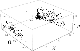
Figure 3: Plot of $\Omega$, $\chi$, and $\mu$. The points within the circle correspond to the best candidates for the ”true“ GRN.

5.1 Concluding remarks and outlook

We have presented a detailed analysis of the problem of GRN inference through the design of a model which captures the biochemical effects between genes and GPs as well as the interaction among the GPs themselves. We hypothesized that the most important role of the GP-GP interaction is to vary (increase or decrease) the characteristic time during which a GP can perform its function. The agreement between data and simulation based on our model suggests that the role of the interaction among GPs is essential in GRNs. To our surprise, the regulation of genes by direct binding of GPs to the genes’ promoters, as described by Eq. (11), amounted to a constant independent of time in all except two clusters, 11 and 12, in the lactose phase. Although one may be tempted to conclude from this result that the transcription rates of nearly all genes are constant in both phases, leaving the non-constant degradation rate in charge of the gene regulation, it should be kept in mind that Eqs (21) and (22) deal with gene clusters, not individual genes. The transcription rates of all genes in a particular cluster may exhibit temporal variations while yielding a constant value when averaged over the cluster. Therefore, our results must be interpreted in the context of cluster network and cannot be directly compared to data on networks containing individual genes.

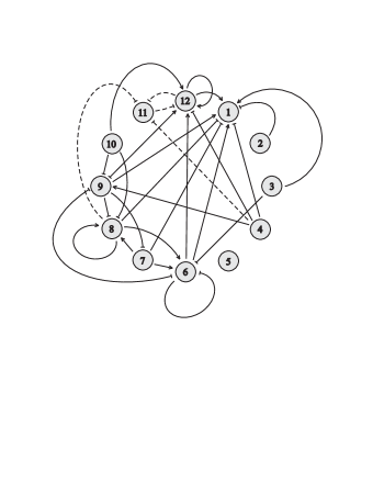
Figure 4: A plausible gene cluster network in the lactose phase based on our criteria. The full lines correspond to the $\kappa^{p}_{q}$’s of Eq. (22) while the dashed lines represent the $\alpha^{p}_{q}$s and $\beta^{p}_{q}$s in Eq. (21).

The cluster network in the lactose phase is very sparse compared to that in the mixed phase. Previous works on the dynamic robustness of GRNs suggests that biological networks with low connectivity are better suited for survival than more densely connected networks [19]. Our results suggest that under external stress, e.g. starvation, the GRN of E. coli becomes highly connected in order to adapt to the suboptimal conditions. This implies that while in the mixed phase, E. coli is more vulnerable to random external perturbations, upon transition to the lactose phase the robustness with respect to environmental insults becomes restored.

The complete connectivity of the mixed phase can also be taken to mean that upon depletion of glucose the different cells try different GRNs, each of which is possibly sparse [20]. Under this assumption, the DNA microarray data would correspond to a superimposition of different GRNs experimented by the system until it finds the right GRN, which allows it to feed on lactose. More experimental and theoretical work will be needed to settle this issue.

Acknowledgements We thank E. Bojilova, T. Konopka, and J. M. Kwasigroch for useful discussions. We acknowledge support from the Belgian State Science Policy Office through an Interuniversity Attraction Poles Programme (DYSCO), and the Belgian Fund for Scientific Research (FNRS) through a FRFC project. MR is Research Director at the FNRS.

References

- [1] T.S Gardner and J.J Faith. Reverse-engineering transcription control networks. Physics of Life Reviews. 2: 65-88 (2005)
- [2] H. Bolouri. Computational Modeling of Gene Regulatory Networks. Imperial College Press. UK (2008)
- [3] H. Lähdesmäki, S. Hautaniemi, I. Shmulevich, O. Y.-Harja. Relationships between probabilistic Boolean networks and dynamic Bayesian networks as models of gene regulatory networks. Signal Processing. 86: 814-834 (2006)
- [4] A. Haye, Y. Dehouck, J. M. Kwasigroch, P. Bogaerts, and M. Rooman. Modeling the temporal evolution of the Drosophila gene expression from DNA microarray time series. Phys. Biol. 6: 016004 (2009)
- [5] J. Gebert, N. Radde, and G.-W. Weber. Modelling gene regulatory networks with piecewise linear differential equations. European Journal of Operational Research. 181: 1148-1165. (2006)
- [6] W. Liebermeister. Linear modes of gene expression determined by independent component analysis. Bioinformatics. 18: 51-60 (2002)
- [7] J. Vohradsky. Neural Model of the Genetic Network. The Journal of Biological Chemistry 276: 39 (2001)
- [8] T.T. Vu and J. Vohradsky. Nonlinear differential equation model for quantification of transcriptional regulation applied to microarray data of Saccharomyces cerevisiae. Nucleic Acid Research. 35: 279-287 (2007)
- [9] A. Krishnan, A. Giuliani, and M. Tomita. Indeterminacy of Reverse Engineering of Gene Regulatory Networks: The Curse of Gene Elasticity. PlosOne. Issue 6: e562 (2007)
- [10] H. Lodish, A. Berk, P. Matsudaira, C. Kaiser, M. Krieger, M. P. Scott, S. L. Zipursky, and J. Darnell. ”Molecular Cell biology.” W. H. Freeman and Company. NY (2004)
- [11] N. E. Buchler, Ulrich Gerland, and Terence Hwa. On schemes of combinatorial transcription logic. PNAS 100 (9): 5136-5141 (2003)
- [12] M. R. Maurizi. Proteases and protein degradation in Escherichia coli. Experientia. 48: 178-201 (1992)
- [13] M. F. Traxler, D-E Chang, and T. Conway. Guanosine 3’,5’-bispyrophosphate coordinates global gene expression during glucose-lactose diauxie in Escherichia coli. Proc. Natl. Acad. Sci. USA. 103(7): 2374-9 (2003)
- [14] P. Smolen, D. E. Baxter, and J. H. Byrne. Frequency selectivity, multistability, and oscillations emerge from models of genetic regulatory systems. Am. J. Physiol. Cell Physiol. 274: 531-542 (1998)
- [15] D. Hekstra, A. R. Taussing, M. Magnasco, and F. Naef. Absolute mRNA concentrations from sequence-specific calibration of oligonucleotide arrays. Nucleic Acids Research. 31(7):1962-1968 (2007)
- [16] B.P. Durbin, J.S. Hardin, D.M. Hawkins, and D.M. Rocke. A variance-stabilizing transformation for gene-expression microarray data. Bioinformatics. 18: S105 (2002)
- [17] R. N. Gutenkunst, J. J. Waterfall, F. P. Casey, K. S. Brown, C. R. Myers, J. P. Sethna. Universally Sloppy Parameter Sensitivities in Systems Biology Models. Plos Computational Biology 3: Issue 10 e189 (2007)
- [18] H. Kitano. Towards a theory of biological robustness. Mol. Syst. Biol. 3: 137 (2007)
- [19] R. D. Leclerc. Survival of the sparsest: robust gene networks are parsimonious. Mol. Syst. Biol. 4: 213 (2008)
- [20] M. Tigges, T. T. Marquez-Lago1, J. Stelling1, and M. Fussenegger. A tunable synthetic mammalian oscillator. Nature 457: 309-312 (2009)