Markovian and non-Markovian dynamics in quantum and classical systems

Abstract

We discuss the conceptually different definitions used for the non-Markovianity of classical and quantum processes. The well-established definition for non-Markovianity of a classical stochastic process represents a condition on the Kolmogorov hierarchy of the $n$-point joint probability distributions. Since this definition cannot be transferred to the quantum regime, quantum non-Markovianity has recently been defined and quantified in terms of the underlying quantum dynamical map, using either its divisibility properties or the behavior of the trace distance between pairs of initial states. Here, we investigate and compare these definitions and their relations to the classical notion of non-Markovianity by employing a large class of non-Markovian processes, known as semi-Markov processes, which admit a natural extension to the quantum case. A number of specific physical examples is constructed which allow to study the basic features of the classical and the quantum definitions and to evaluate explicitly the measures for quantum non-Markovianity. Our results clearly demonstrate several fundamental distinctions between the classical and the quantum notion of non-Markovianity, as well as between the various quantum measures for non-Markovianity.

I Introduction

A lot of effort has been put into the study and understanding of non-Markovian effects and dynamics within the description of open quantum systems Breuer2002 (1). These efforts have faced quite a huge amount of difficulties arising both because of practical as well as fundamental reasons. Indeed, on the one hand the treatment of non-Markovian systems is especially demanding because one cannot rely on simplifying assumptions such as weak coupling, separation of time scales between system and environment, and the factorization of the system-environment state. On the other hand, in the non-Markovian case there is no general characterization of the equations of motion, such as in the Markovian setting thanks to the theory of quantum dynamical semigroups, and the very notion of non-Markovianity in the quantum case still has to be cleared up. In the last few years this topic has experienced a significant revival, leading to important improvements and to the deeper understanding of quite a few issues in the theory of open quantum systems (see e.g. Stockburger2002a (2, 3, 4, 5, 6, 7, 8, 9) and references therein).

Apart from the explicit detailed treatment of many specific quantum systems where memory effects show up, efforts have been made to obtain general classes of non-Markovian equations leading to well-defined completely positive time evolutions Budini2004a (10, 5). At the same time advances have been made in order to actually define what is meant by a non-Markovian quantum dynamics Wolf2008a (11, 12, 13). This work has raised all sorts of questions regarding the connection among the different approaches, as well as the relationship between the notion of non-Markovianity used in classical and quantum setting, together with the quest for clearcut signatures of non-Markovian behavior.

The present paper is devoted to address some of these questions, focussing in particular on the connection between the very definition of non-Markovian process used in classical probability theory, and the Markovian or non-Markovian behavior in the dynamics of a physical system. It will naturally appear that these two notions are quite different. Starting within the classical framework, we will analyze how the non-Markovianity of a process reflects itself in the behavior of its one-point probability density, which naturally leads to criteria for the characterization of non-Markovian behavior in the dynamics. These criteria can be extended to the quantum setting, thus providing natural tools to assess the non-Markovianity of a quantum time evolution. They are based on the possibility to connect the probability vectors giving the state of the system at different times through well defined transition matrices, and to the behavior of solutions corresponding to different initial states with respect to the Kolmogorov distance.

Despite the abstract framework, the whole presentation is built with reference to explicit examples. These examples find their common root in being related to realizations of a class of non-Markovian processes for which, as an exceptional case, an explicit characterization is available, namely semi-Markov processes. This approach will enable us to construct different non trivial dynamics both in the classical and the quantum case, showing quite different behaviors and amenable to an explicit analysis, both in terms of the previously introduced criteria and of the recently proposed measures of non-Markovianity, thus allowing for a concrete comparison of these measures.

The paper is organized as follows. In Sect. II we introduce the notion of classical and quantum map for the dynamics of an open system, introducing the notions of P-divisibility and CP-divisibility which will turn out to be useful in order to compare different behaviors. In Sect. III we recall the notion of non-Markovianity for a classical process, showing its relation to the behavior of the one-point probability density. We further consider examples of classical semi-Markov processes characterized by different stochastic matrices and waiting time distributions, studying their P-divisibility and the behavior with respect to the Kolmogorov distance. In Sect. IV we perform a similar analysis in the quantum setting, considering classes of dynamics which can be related to semi-Markov processes. These dynamics still allow for an exact determination of their divisibility properties and of their quantum measure of non-Markovianity according to the recent proposals. In particular we provide exact expressions for the values of these measures, thus allowing for their explicit comparison. We further comment on our results in Sect. V.

II Dynamical maps

If the initial state of system and environment factorizes, the dynamics of an open quantum system can be described by a trace preserving completely positive (CPT) map, so that the state of the system $\rho\left(t\right)$ evolving from an initial state $\rho\left(t_{0}\right)$ is given by

$$\rho\left(t\right) = \Phi\left(t,t_{0}\right)\rho\left(t_{0}\right).$$ (1)

The most general structure of such time evolution maps is not known, apart from the important subclass of maps which obey a semigroup composition law, which can be characterized via a suitable generator Lindblad1976a (14, 15). In order to characterize and actually define Markovianity or non-Markovianity in this setting one can follow essentially two approaches: either one assumes that the map $\Phi\left(t,t_{0}\right)$ is known, and therefore relys on looking at certain mathematical properties of the map itself, which is essentially the path followed in different ways in Wolf2008a (11, 13); or one studies the behavior in time of the solutions $\rho\left(t\right)$ allowing the initial condition to vary over the possible set of states, which is the approach elaborated in Breuer2009b (12, 16) relying on a suitable notion of distinguishability of quantum states Hayashi2006 (17), an approach which captures the idea of information flow between system and environment. Note that Markovianity or non-Markovianity should be a property of the map or equivalently of the time evolved states, not of the equations admitting such states as solutions. Indeed quite different form of the equations, e.g. integrodifferential or local in time, might admit the very same solutions, as we shall also see in the examples in Sect. IV. Of course, since in a concrete physical setting one is rather faced with the equations of motion rather than with their general solution, it is therefore also of great interest to assess possible links between the equations themselves and the Markovian or non-Markovian behavior of their solutions.

To better understand and compare these two approaches, besides the notion of complete positivity and trace preservation other finer characterizations of the time evolution map $\Phi\left(t,0\right)$ turn out to be useful, where we have set for the sake of simplicity $t_{0}=0$. If the map $\Phi\left(t,0\right)$ can be split according to

$$\Phi\left(t,0\right) = \Phi\left(t,s\right)\Phi\left(s,0\right)$$ (2)

for any $t\geqslant s\geqslant 0$, with $\Phi\left(t,s\right)$ itself a CPT map, we say that the map $\Phi\left(t,0\right)$ is CP-divisible, which implies that $\Phi\left(t,s\right)$ is itself a well-defined time evolution having as domain the whole set of states. Note that at variance with Ref. Wolf2008b (18) focussing on quantum channels, the notion of divisibility considered here refers to families of time dependent dynamical maps. The existence of $\Phi\left(t,s\right)$ as a linear map is granted if $\Phi\left(s,0\right)$ is invertible, which is typically the case away from isolated points of time, so that

$$\Phi\left(t,s\right) = \Phi\left(t,0\right)\Phi^{-1}\left(s,0\right).$$ (3)

The existence of $\Phi\left(t,s\right)$ as a linear map, however, does not entail its complete positivity. Indeed, we will say that the map $\Phi\left(t,0\right)$ is P-divisible if $\Phi\left(t,s\right)$ send states into states but is only positive, and that it is indivisible if neither P-divisibility nor CP-divisibility hold. Examples of such maps together with their physical interpretation will be provided in Sect. IV.

The notion of P-divisibility can be considered also in the classical setting. Suppose to consider a finite dimensional classical system, described by a probability vector $\boldsymbol{p}\left(t\right)$. Its time evolution can be described by a time dependent collection of stochastic matrices $\Lambda\left(t,0\right)$ according to

$$\boldsymbol{p}\left(t\right) = \Lambda\left(t,0\right)\boldsymbol{p}\left(0\right).$$ (4)

Similarly as before, we say that the classical map $\Lambda\left(t,0\right)$ is P-divisible provided for any $t\geqslant s\geqslant 0$ one can write

$$\Lambda\left(t,0\right) = \Lambda\left(t,s\right)\Lambda\left(s,0\right),$$ (5)

where each of the $\Lambda\left(t,s\right)$ is itself a stochastic matrix. Its matrix elements satisfy therefore $\left(\Lambda\left(t,s\right)\right)_{ij}\geqslant 0$ and $\sum_{k}\left(\Lambda\left(t,s\right)\right)_{kj}=1$, which provide the necessary and sufficient conditions ensuring that probability vectors are sent into probability vectors Norris1999 (19). Once again this need not generally be true, even if the map $\Lambda\left(s,0\right)$ is invertible as linear operator. Note that we are here only considering the one-point probabilities $\boldsymbol{p}\left(t\right)$, which are certainly not enough to assess Markovianity or non-Markovianity of a process according to the mathematically precise definition used in classical probability theory.

III Classical non-Markovian processes

Let us now recall what is the very definition of non-Markovian process in the classical probabilistic setting.  Indeed the analysis of classical processes is a natural starting point, also adopted in Chruscinski2010c (20, 21, 22, 23, 24). Suppose we are considering a stochastic process taking values in a numerable set $\left\{x_{i}\right\}_{i\in\mathbbm{N}}$. The process is said to be Markovian if the conditional transition probabilities satisfy

$$p_{1|n}\left(x_{n},t_{n}|x_{n-1},t_{n-1};\ldots;x_{0},t_{0}\right)=\\ p_{1|1}\left(x_{n},t_{n}|x_{n-1},t_{n-1}\right)$$ (6)

with $t_{n}\geqslant t_{n-1}\geqslant\ldots\geqslant t_{1}\geqslant t_{0}$, so that the probability that the random variable assumes the value $x_{n}$ at time $t_{n}$, given that it has assumed given values $x_{i}$ at previous times $t_{i}$, actually only depends on the last assumed value, and not on previous ones. In this sense the process is said to lack memory. This statement obviously involves all $n$-times probabilities, so that the non-Markovianity of the process cannot be assessed by looking at the one-time probabilities only VanKampen1998a (25, 26). It immediately appears from Eq. (6) that such a definition cannot be transferred to the quantum realm, since the very notion of conditional probability does depend on the measurement performed in order to ascertain the previous value of the random variable, and on how it transforms the state for the subsequent time evolution.

If we know that the process is Markovian the $n$-point probabilities can be easily obtained in terms of the initial probability density and the conditional transition probability $p_{1|1}$ according to

$$p_{n}\left(x_{n},t_{n};x_{n-1},t_{n-1};\ldots;x_{0},t_{0}\right)=\\ \prod_{i=1}^{n}p_{1|1}\left(x_{i},t_{i}|x_{i-1},t_{i-1}\right)p_{1}\left(x_{0},t_{0}\right).$$ (7)

The Markov condition Eq. (6) in turn implies that the conditional transition probability $p_{1|1}$ obeys the Chapman-Kolmogorov equation

$$p_{1|1}\left(x,t|y,s\right) = \sum_{z}p_{1|1}\left(x,t|z,\tau\right)p_{1|1}\left(z,\tau|y,s\right),$$ (8)

with $t\geqslant\tau\geqslant s$, whose possible solutions characterize the transition probabilities of a Markov process. A Markov process is therefore uniquely characterized by its conditional transition probability and the initial distribution.

If $\boldsymbol{p}\left(t\right)$ denotes the vector giving the one-point probability of a Markov process taking values in a finite space, and if $\Lambda\left(t,s\right)$ is its conditional transition probability expressed in matrix form, the probability vectors at different times are related according to

$$\boldsymbol{p}\left(t\right) = \Lambda\left(t,s\right)\boldsymbol{p}\left(s\right)$$ (9)

with $t\geqslant s\geqslant 0$ and $\Lambda\left(t,s\right)$ a stochastic matrix obeying the Chapman-Kolmogorov equation, which in this case is equivalent to the requirement of P-divisibility in the sense of Eq. (5). However, in general validity of the Chapman-Kolmogorov equation and P-divisibility obviously do not coincide, since the P-divisibility does not tell anything about the higher-point conditional probabilities. Indeed, for a given process one might find a matrix $\Lambda\left(t,s\right)$ satisfying Eq. (9) even if the process is non-Markovian, however in this case the matrix is not the conditional transition probability of the process Hanggi1977a (27, 28). Similarly to Eq. (3), if $\Lambda\left(t,0\right)$ is invertible one can obtain such a matrix as

$$\Lambda\left(t,s\right) = \Lambda\left(t,0\right)\Lambda^{-1}\left(s,0\right),$$ (10)

which warrants independence from the initial probability vector. On the contrary, the conditional transition probability of a non-Markovian process does depend on the initial probability vector Hanggi1977a (27).

III.1 Classical semi-Markov processes

To spell out this situation in detail let us consider an example. The main difficulty lies in the fact that generally very little is known on non-Markovian processes. We will however consider a class of non-Markovian processes allowing for a compact characterization, that is to say semi-Markov processes Feller1971 (29). To this end we consider a system having a finite set of states, which can jump from one state to the other according to certain jump probabilities $\pi_{mn}$, waiting a random time in each state before jumping to the next. Such a process turns out to be Markovian if and only if the waiting time distributions $f_{n}\left(\tau\right)$ characterizing the random sojourn time spent in each state are given by exponential probability distributions, and non-Markovian otherwise. Each such process is fixed by its semi-Markov matrix

$$\left(Q\right)_{mn}\left(\tau\right) = \pi_{mn}f_{n}\left(\tau\right),$$ (11)

where the $\pi_{mn}$ are the elements of a stochastic matrix. Assuming for the sake of simplicity a two-dimensional system, a site independent waiting time distribution and the stochastic matrix to be actually bistochastic Norris1999 (19), the semi-Markov matrix is determined according to

$$Q\left(\tau\right) = \left(\begin{array}[]{cc}1-\pi&\pi\\ \pi&1-\pi\end{array}\right)f\left(\tau\right),$$ (14)

$$\equiv \Pi f\left(\tau\right)$$ (15)

with $\pi$ a positive number between zero and one giving the probability to jump from one site to the other, and $f\left(\tau\right)$ an arbitrary waiting time distribution with associated survival probability

$$g\left(t\right) = 1-\int_{0}^{t}\mathrm{d}\tau f\left(\tau\right).$$ (16)

III.2 Transition probability

The transition probability for such a process can be determined exploiting the fact that it is known to obey the following integrodifferential Kolmogorov forward equation Feller1964a (31)

$$\frac{\mathrm{d}}{\operatorname{dt}}T\left(t,0\right) = \int_{0}^{t}\mathrm{d}\tau W\left(\tau\right)T\left(t-\tau,0\right),$$ (17)

here expressed in matrix form with

$$W\left(\tau\right) = \left(\Pi-\mathbbm{1}\right)k\left(\tau\right),$$ (18)

where the memory kernel $k\left(\tau\right)$ relates waiting time distribution and survival probability according to

$$f\left(\tau\right) = \int_{0}^{\tau}\mathrm{d}tk\left(\tau-t\right)g\left(t\right).$$ (19)

Denoting by $\hat{v}\left(u\right)$ the Laplace transform of a function or matrix $v\left(\tau\right)$ according to

$$\hat{v}\left(u\right) = \int^{+\infty}_{0}\mathrm{d}\tau v\left(\tau\right)\mathrm{e}^{-u\tau},$$ (20)

the solution of this equation with initial condition $T\left(0,0\right)=\mathbbm{1}$ can be expressed as

$$\hat{T}\left(u\right) = \frac{\hat{g}\left(u\right)}{\mathbbm{1}-\Pi\hat{f}\left(u\right)}.$$ (21)

III.3 Explicit examples

The explicit solution of Eq. (21) for $\pi=1/2$, so that at each step the system has equal probability to remain in the same site or change, is given by

$$T\left(t,0\right) = \frac{1}{2}\left(\begin{array}[]{cc}1+g\left(t\right)&1-g\left(t\right)\\ 1-g\left(t\right)&1+g\left(t\right)\end{array}\right),$$ (24)

so that according to Eq. (10) we can introduce the matrices

$$T\left(t,s\right) = T\left(t,0\right)T^{-1}\left(s,0\right)$$ (27)

$$= \frac{1}{2}\left(\begin{array}[]{cc}1+g\left(t\right)/g\left(s\right)&1-g\left(t\right)/g\left(s\right)\\ 1-g\left(t\right)/g\left(s\right)&1+g\left(t\right)/g\left(s\right)\end{array}\right),$$

which indeed connect the probability vectors at different times according to

$$\boldsymbol{p}\left(t\right) = T\left(t,s\right)\boldsymbol{p}\left(s\right).$$ (28)

Given the fact that for any non vanishing waiting time distribution the survival probability is a strictly positive monotonic decreasing function, the matrices $T\left(t,s\right)$ are well-defined stochastic matrices for any pair of times $t\geqslant s$, so that the classical map $T\left(t,0\right)$ is always P-divisible, irrespective of the fact that the underlying process is Markovian only for the special choice of an exponential waiting time distribution of the form

$$f\left(\tau\right) = \lambda\mathrm{e}^{-\lambda\tau}.$$ (29)

This result implies that the one-point probabilities of the considered non-Markovian semi-Markov process can be equally well obtained from a Markov process with conditional transition probability $p_{1|1}$ given by $T$, whose $n$-point probabilities can be obtained as in Eq. (7). The latter would however differ from those of the considered semi-Markov process.

As a complementary situation, let us consider the case $\pi=1$, so that once in a state the system jumps with certainty to the other, thus obtaining as explicit solution of Eq. (21) the expression

$$T\left(t,0\right) = \frac{1}{2}\left(\begin{array}[]{cc}1+q\left(t\right)&1-q\left(t\right)\\ 1-q\left(t\right)&1+q\left(t\right)\end{array}\right),$$ (32)

and therefore

$$T\left(t,s\right) = T\left(t,0\right)T^{-1}\left(s,0\right)$$ (35)

$$= \frac{1}{2}\left(\begin{array}[]{cc}1+q\left(t\right)/q\left(s\right)&1-q\left(t\right)/q\left(s\right)\\ 1-q\left(t\right)/q\left(s\right)&1+q\left(t\right)/q\left(s\right)\end{array}\right).$$

The quantity $q\left(t\right)$ appearing in these matrices is the inverse Laplace transform of the function

$$\hat{q}\left(u\right) = \frac{1}{u}\frac{1-\hat{f}\left(u\right)}{1+\hat{f}\left(u\right)}.$$ (36)

Recalling that the probability for $n$ jumps in a time $t$ for a waiting time distribution $f\left(t\right)$ is given by

$$p_{n}\left(t\right)=\int^{t}_{0}\mathrm{d}\tau f\left(t-\tau\right)p_{n-1}\left(\tau\right),$$ (37)

so that

$$\hat{p}_{n}\left(u\right) = \hat{p}_{0}\left(u\right)\hat{f}^{n}\left(u\right),$$ (38)

one has

$$q\left(t\right) = \sum^{\infty}_{n=0}p_{2n}(t)-\sum^{\infty}_{n=0}p_{2n+1}(t)$$

$$= p_{\operatorname{even}}\left(t\right)-p_{\operatorname{odd}}\left(t\right).$$

The quantity $q\left(t\right)$ therefore expresses the difference between the probability to have an even or an odd number of jumps. At variance with the previous situation, the quantity $q\left(t\right)$ depending on the waiting time distribution can assume quite different behavior, showing oscillations and going through zero at isolated time points, so that at these time points, corresponding to a crossing of trajectories starting from different initial conditions, the transition matrix $T\left(t,s\right)$ is not defined. Moreover due to the non monotonicity of $q\left(t\right)$ the matrices $T\left(t,s\right)$ cannot always be interpreted as stochastic matrices. Of course in the Markovian case, corresponding to Eq. (29) and therefore to $q\left(t\right)=\exp\left(-2\lambda t\right)$, all these features are recovered.

The variety of possible behaviour is best clarified by considering explicit expressions for the waiting time distribution $f\left(t\right)$ which determines the process once the stochastic matrix $\Pi$ is given. Quite general expressions of waiting time distribution can be obtained by considering convex mixtures or convolutions of exponential waiting time distributions with equal or different parameters, whose Laplace transform is given by rational functions Cox1965 (32, 33). To better understand the dynamics generated by the maps Eq. (24) and Eq. (32) in the following examples note that for  $\pi=1/2$ the matrix $\Pi$ is idempotent, sending each probability vector to the uniform distribution, while for $\pi=1$ one has $\Pi^{2n}=\mathbbm{1}$, and the action of the bistochastic matrix consists in swapping the two elements of the probability vector.

III.3.1 Convolution of exponential waiting time distributions

The behavior of the quantity $q\left(t\right)$ can be explicitly assessed for the case of a waiting time distribution $\mathsf{f}\left(t\right)$ given by the convolution of two exponential waiting time distributions. Let us first consider the case in which the waiting time distributions share the same parameter $\lambda$, so that $\mathsf{f}=f\ast f$ with $f$ as in Eq. (29), corresponding to

$$\mathsf{f}\left(t\right) = \lambda^{2}t\mathrm{e}^{-\lambda t}$$ (40)

and therefore

$$\mathsf{g}\left(t\right) = \left(1+\lambda t\right)\mathrm{e}^{-\lambda t}.$$ (41)

This is a special case of the Erlang distribution Medhi1994 (33), leading to

$$q\left(t\right) = \mathrm{e}^{-\lambda t}\left[\cos\left(\lambda t\right)+\sin\left(\lambda t\right)\right],$$ (42)

which oscillates and crosses zero at isolated points, so that the matrices $T\left(t,s\right)$ are not defined at these points and cannot be always interpreted as stochastic matrices, since their entries can become negative. This behavior is exhibited in Fig. 1

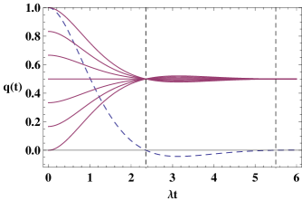
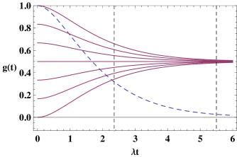
Figure 1: (Color online) (top) Plot of the function $q$ (dashed line) given by Eq. (III.3) as a function of $\lambda t$ for the convolution of two equal exponential waiting time distributions, for the case of a semi-Markov process with $\pi=1$, together with a few trajectories (continuous lines) for the upper element $w\left(t\right)$ of the one-point probability according to Eq. (45). The initial data $w\left(0\right)$ are uniformly taken between 0 and 1. When $q\left(t\right)$ goes through zero the trajectories cross. At these points $\left|q\left(t\right)\right|$ starts growing, which indicates the failure of P-divisibility of the time evolution as defined in Eq. (5). (bottom) Plot of the function $g$  given by Eq. (16) as a function of $\lambda t$, for the same waiting time distribution, together with a few trajectories, corresponding to a semi-Markov process with $\pi=1/2$. As it appears, despite sharing the same waiting time distribution the trajectories for this semi-Markov process never cross, and P-divisibility holds even if the process is non-Markovian.

, where the quantity Eq. (42) is plotted together with the trajectories of the probability vector with different initial conditions. We also consider the behavior of $\mathsf{g}\left(t\right)$ and of the trajectories for the same waiting time distribution but a semi-Markov process with stochastic matrix fixed by $\pi=1/2$. The probability vector is of the form

$$\boldsymbol{p}\left(t\right) = \left(\begin{array}[]{c}w\left(t\right)\\ 1-w\left(t\right)\end{array}\right),$$ (45)

so that its trajectories are displayed showing $w\left(t\right)$, where

$$w\left(t\right) = \frac{1}{2}\left[1-q\left(t\right)+2q\left(t\right)w\left(0\right)\right]$$ (46)

or

$$w\left(t\right) = \frac{1}{2}\left[1-\mathsf{g}\left(t\right)+2\mathsf{g}\left(t\right)w\left(0\right)\right]$$ (47)

in the two cases $\pi=1$ and $\pi=1/2$ respectively. Note how for $\pi=1$ the different trajectories tend to group together and then separate again depending on the behaviour of $q\left(t\right)$. A more general situation is given by $\mathsf{f}=f_{1}\ast f_{2}$, where each $f_{i}$ is of the form Eq. (29) with parameter $\lambda_{i}$, so that one has

$$\mathsf{f}\left(t\right) = 2\frac{p}{s}\mathrm{e}^{-\frac{1}{2}st}\frac{1}{\xi}\operatorname{Sinh}\left(\frac{st}{2}\xi\right)$$ (48)

and correspondingly

$$\mathsf{g}\left(t\right) = \mathrm{e}^{-\frac{1}{2}st}\left[\operatorname{Cosh}\left(\frac{st}{2}\xi\right)+\frac{1}{\xi}\operatorname{Sinh}\left(\frac{st}{2}\xi\right)\right],$$ (49)

where we have set

$$s = \lambda_{1}+\lambda_{2}$$

$$p = \lambda_{1}\lambda_{2}$$

$$\xi = \sqrt{1-4\frac{p}{s^{2}}}.$$ (50)

The function $q\left(t\right)$ determining the matrices $T\left(t,s\right)$ is now given by

$$q\left(t\right) = \mathrm{e}^{-\frac{1}{2}st}\left[\operatorname{Cosh}\left(\frac{st}{2}\chi\right)+\frac{1}{\chi}\operatorname{Sinh}\left(\frac{st}{2}\chi\right)\right]$$ (51)

with

$$\chi = \sqrt{1-8\frac{p}{s^{2}}}.$$ (52)

The expression given by Eq. (51) shows an oscillatory behaviour if $\chi$ becomes imaginary, for $3-2\sqrt{2}\leqslant\lambda_{1}/\lambda_{2}\leqslant 1/\left(3-2\sqrt{2}\right)$, while it is a positive monotonic function of $t$ otherwise. The latter situation is considered in Fig. 2

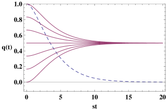
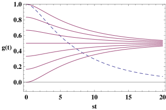
Figure 2: (Color online) (top) Plot of the function $q\left(t\right)$ (dashed line) and of the trajectories (continuous lines) as in Fig. 1, but for the convolution of two different exponential waiting time distributions. We plot $q$ as a function of $st$, taking $p/s^{2}=0.12$, with $s$ and $p$ sum and product of the two parameters characterizing the exponential waiting time distributions as in Eq. (50). For this case the quantity $\chi$ given by Eq. (52) is positive, ensuring monotonicity of $q\left(t\right)$. (bottom) Plot of $g\left(t\right)$ and the corresponding trajectories for the same waiting time distribution.

.

III.3.2 Mixture of exponential waiting time distributions

For the case of a convex mixture of two exponential distributions on the contrary the trajectories never cross, and the matrices $T\left(t,s\right)$ always are well-defined stochastic matrices. Indeed this can be seen from

$$\mathsf{f}\left(t\right) = \mu f_{1}\left(t\right)+\left(1-\mu\right)f_{2}\left(t\right),$$ (53)

with $0\leqslant\mu\leqslant 1$, so that

$$\mathsf{g}\left(t\right) = \mu\mathrm{e}^{-\lambda_{1}t}+\left(1-\mu\right)\mathrm{e}^{-\lambda_{2}t}$$ (54)

and

$$q\left(t\right) =\mathrm{e}^{-\frac{1}{2}\left(\lambda_{1}+\lambda_{2}+\langle\lambda\rangle\right)t}$$ (55)

$$\hphantom{=}\times\left[\operatorname{Cosh}\left(\frac{\bar{\lambda}t}{2}\right)+\frac{\left(\lambda_{1}+\lambda_{2}-3\langle\lambda\rangle\right)}{\bar{\lambda}}\operatorname{Sinh}\left(\frac{\bar{\lambda}t}{2}\right)\right],$$

with

$$\langle\lambda\rangle = \mu\lambda_{1}+\left(1-\mu\right)\lambda_{2}$$ (56)

the mean rate and

$$\bar{\lambda} = \sqrt{\left(\lambda_{1}+\lambda_{2}+\langle\lambda\rangle\right)^{2}-8\lambda_{1}\lambda_{2}}.$$ (57)

This case is considered in Fig. 3

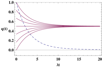
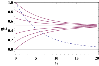
Figure 3: (Color online) (top) Plot of $q\left(t\right)$ (dashed line) and the trajectories (continuous lines) as in Fig. 1, but for the convex mixture of two different exponential waiting time distributions. We plot $q$ as as a function of $\lambda t$, taking $\lambda_{1}=a_{1}\lambda$ and $\lambda_{2}=a_{2}\lambda$, with $a_{1}=.1$ and $a_{2}=.2$, together with mixing parameter $\mu=0.3$. (bottom) Plot of $g\left(t\right)$ and the corresponding trajectories for the same waiting time distribution.

.

It should be noticed that in all these situations the process is non-Markovian, but P-divisibility of the time evolution $\Lambda\left(t,0\right)$ in the sense of Eq. (5) still holds in some cases. For a semi-Markov process with semi-Markov matrix as in Eq. (14) and $\pi=1/2$, P-divisibility always holds, in particular as shown in the examples the trajectories never cross and $\left|q\left(t\right)\right|$ never grows. For $\pi=1$ on the contrary the behaviour depends on the waiting time distribution, which determines whether or not the quantity $q\left(t\right)$ shows an oscillating behavior, implying that the trajectories start getting closer till they cross and then get apart once again.

III.4 Kolmogorov distance

It is interesting to relate this behavior to the time dependence of the Kolmogorov distance among probability distributions arising from different initial states. The Kolmogorov distance between two probability vectors can be written as Fuchs1999a (34, 35)

$$D_{K}\left(\boldsymbol{p}^{1}\left(t\right),\boldsymbol{p}^{2}\left(t\right)\right) = \frac{1}{2}\sum_{i}\left|p_{i}^{1}\left(t\right)-p_{i}^{2}\left(t\right)\right|.$$ (58)

If the map $\Lambda\left(t,0\right)$ is P-divisible in the sense of Eq. (5), then the Kolmogorov distance is a monotonic decreasing function of time. Indeed by the two basic properties of a stochastic matrix, the positivity of its entries and the fact that each row sum up to one, one has for $t\geqslant s\geqslant 0$

$$D_{K}\left(\boldsymbol{p}^{1}\left(t\right),\boldsymbol{p}^{2}\left(t\right)\right) = \frac{1}{2}\sum_{i}\left|\sum_{k}\Lambda\left(t,s\right)_{ik}\left(\boldsymbol{p}^{1}\left(s\right)-\boldsymbol{p}^{2}\left(s\right)\right)_{k}\right|$$ (59)

$$\leqslant \frac{1}{2}\sum_{i}\sum_{k}\Lambda\left(t,s\right)_{ik}\left|\left(\boldsymbol{p}^{1}\left(s\right)-\boldsymbol{p}^{2}\left(s\right)\right)_{k}\right|$$

$$= \frac{1}{2}\sum_{k}\left|\left(\boldsymbol{p}^{1}\left(s\right)-\boldsymbol{p}^{2}\left(s\right)\right)_{k}\right|$$

$$= D_{K}\left(\boldsymbol{p}^{1}\left(s\right),\boldsymbol{p}^{2}\left(s\right)\right).$$

This holds true independently of the fact that the underlying classical process is Markovian or not, it only depends on the fact the one-point probabilities can be related at different times via stochastic matrices.

In a generic non-Markovian situation the Kolmogorov distance can both show a monotonic decreasing behavior as well as revivals. Indeed, focusing on the examples considered above, for a semi-Markov matrix as in Eq. (14) and $\pi=1/2$ one has

$$D_{K}\left(\boldsymbol{p}^{1}\left(t\right),\boldsymbol{p}^{2}\left(t\right)\right) = g\left(t\right)D_{K}\left(\boldsymbol{p}^{1}\left(0\right),\boldsymbol{p}^{2}\left(0\right)\right),$$ (60)

while for $\pi=1$ one has

$$D_{K}\left(\boldsymbol{p}^{1}\left(t\right),\boldsymbol{p}^{2}\left(t\right)\right) = \left|q\left(t\right)\right|D_{K}\left(\boldsymbol{p}^{1}\left(0\right),\boldsymbol{p}^{2}\left(0\right)\right).$$ (61)

Thus, while for $\pi=1/2$ the Kolmogorov distance is a monotonic contraction for any waiting time distribution, thanks to the fact that $g\left(t\right)$ is a survival probability, for $\pi=1$ the distance among distributions can show revivals depending on the explicit expression of $q\left(t\right)$, as can be seen from Fig. 1 for the case of the convolution of two exponential waiting time distributions with the same parameter.

We have thus studied, by means of explicit examples, the behavior of the probability vector or one-point probability $\boldsymbol{p}\left(t\right)$ of a classical process. In particular, we have seen that while for a Markovian process P-divisibility is always granted and the Kolmogorov distance is a monotone contraction, non-Markovianity can spoil these features, even though neither the lack of P-divisibility nor the growth of the Kolmogorov distance can be taken as necessary signatures of non-Markovianity. This is not surprising due to the fact that the non-Markovianity of a classical process cannot be traced back to the behavior of the one-point probabilities, since it involves all $n$-point probabilities.

IV Quantum non-Markovian processes

We now come back to the quantum realm, studying a class of quantum dynamics which have a clearcut physical meaning, allowing both for the evaluation and the comparison of two recently introduced measures of non-Markovianity for the quantum case, and for a direct connection with the classical situation analyzed in Sect. III. Indeed, while in the classical case one has a well settled definition of non-Markovianity for a stochastic process, which can be used to speak of Markovianity or non-Markovianity of the time evolution of the associated probability distributions, equivalent characterizations for the quantum case have been proposed only recently. As follows from the discussion in Sect. III, such approaches cope by necessity with the behavior of the one-point probabilities only, which can be obtained from the statistical operator $\rho\left(t\right)$, since a definition involving the whole hierarchy of $n$-point probabilities cannot be introduced without explicit reference to a particular choice of measurement scheme. Note that in the study of quantum dynamics one speaks about measures of non-Markovianity, since apart from clarifying what is the signature of non-Markovianity, so as to define it and therefore make it detectable, one would like to quantify the degree of non-Markovianity of a given dynamics.

The two measures that we will consider here Breuer2009b (12, 13) actually respectively rely on the violation of the quantum analog of the classical properties of P-divisibility and monotonic decrease in time of the Kolmogorov distance, that we have considered in Sect. III and hold true for the Markovian case, while also other approaches have been considered Wolf2008a (11). Note that the violation of these properties in the classical case provide a sufficient but not necessary condition to detect a non-Markovian process, as clarified in the examples considered in Sect. III.1.

IV.1 Quantum semi-Markov processes

As in the classical case, in order to study the Markovian or non-Markovian features of a quantum dynamics we consider a class of time evolutions which allow for an explicit treatment and the connection to a classical counterpart. Let us study dynamics given by master equations of the form Budini2004a (10)

$$\frac{\mathrm{d}}{\operatorname{dt}}\rho\left(t\right) = \int^{t}_{0}d\tau k\left(t-\tau\right)\left[\mathcal{E}-\mathbbm{1}\right]\rho\left(\tau\right),$$ (62)

where $\mathcal{E}$ is a CPT map and $k\left(t\right)$ a memory kernel associated to a waiting time distribution $f\left(t\right)$ according to Eq. (19). Such master equations generate by construction completely positive dynamics, which provide a quantum counterpart of classical semi-Markov processes Breuer2008a (5, 30). Indeed, as it can be checked, the solution of Eq. (62) can be written as

$$\rho\left(t\right) = \Phi\left(t,0\right)\rho\left(0\right)$$ (63)

$$= \sum^{\infty}_{n=0}p_{n}(t)\mathcal{E}^{n}\rho\left(0\right),$$

with $p_{n}(t)$ fixed by $f\left(t\right)$ according to Eq. (37), while $\mathcal{E}^{n}$ denotes the $n$-fold composition of the map $\mathcal{E}$. The map $\Phi\left(t,0\right)$ is thus completely positive by construction and can be interpreted as the repeated action of the CPT map $\mathcal{E}$, implementing a quantum operation, distributed in time according to the waiting time distribution $f\left(t\right)$. For the case of an exponential waiting time distribution the memory kernel is a delta function and one goes back to a semigroup dynamics. In Sect. III we considered semi-Markov processes with a semi-Markov matrix of the form Eq. (14), with arbitrary $f\left(t\right)$ and $\Pi$ a bistochastic matrix, and where Markovianity or non-Markovianity of the process depended only on the choice of $f\left(t\right)$, while P-divisibility and behavior of the Kolmogorov distance did depend on both $f\left(t\right)$ and $\Pi$. In the quantum setting we also leave $f\left(t\right)$ arbitrary and consider bistochastic CPT maps, in the sense that $\mathcal{E\left[\mathbbm{1}\right]=}\mathbbm{1}$, so that also $\Phi\left(t,0\right)$ is bistochastic, preserving both the trace and the identity.

IV.2 Dephasing dynamics and time-local equation

A purely quantum dynamics, only affecting coherences, is obtained considering the CPT map

$$\mathcal{E}_{z}\rho = \sigma_{z}\rho\sigma_{z},$$ (64)

which satisfies $\mathcal{E}_{z}^{2n}=\mathbbm{1}$ and $\mathcal{E}_{z}^{2n+1}=\mathcal{E}_{z}$, so that one has

$$\rho\left(t\right) = p_{\operatorname{even}}\left(t\right)\rho\left(0\right)-p_{\operatorname{odd}}\left(t\right)\sigma_{z}\rho\left(0\right)\sigma_{z}$$ (65)

$$= \left(\begin{array}[]{cc}\rho_{11}(0)&q(t)\rho_{10}(0)\\ q(t)\rho_{01}(0)&\rho_{00}(0)\end{array}\right),$$ (68)

recalling the definition Eq. (III.3) of $q\left(t\right)$ and considering matrix elements in the basis of eigenvectors of $\sigma_{z}$. Before addressing the issue of characterization of these dynamics, it is of interest to recast the integrodifferential master equation Eq. (62) in a time-convolutionless form. Indeed, while Markovianity or non-Markovianity is a property of the solution $\rho\left(t\right)$, rather then of the equation, it is quite important to read the signatures of a non-Markovian behavior from the equations themselves, and this task turns out to be much easier when the equations are written in time-local form. To rewrite the master equation Eq. (62) in time-local form we follow the constructive approach used in Smirne2010b (36). We thus obtain the time-convolutionless generator, which is formally given by $\dot{\Phi}\left(t,0\right)\Phi^{-1}\left(t,0\right)$, by a representation of the map as a matrix with respect to a suitable operator basis in $\mathbbm{C}^{2}$, given by $\left\{X_{i}\right\}=\left\{\frac{1}{\sqrt{2}}\mathbbm{1},\frac{1}{\sqrt{2}}\sigma_{i}\right\}_{i=1,2,3}$, orthonormal according to $\operatorname{Tr}_{S}\left\{X_{i}X_{j}\right\}=\delta_{ij}$. The matrix $F=\left(F_{kl}\right)$ associated to the map $\Phi$ is then determined as

$$F_{kl} = \operatorname{Tr}_{S}\left\{X^{{\dagger}}_{k}\Phi\left[X_{l}\right]\right\},$$

so that

$$\Phi\left[\rho\right] = \sum_{kl}F_{kl}\operatorname{Tr}_{S}\left\{X_{l}^{{\dagger}}\rho\right\}X_{k}.$$

The matrix $F$ for our map is given by

$$F\left(t,0\right) = \operatorname{diag}\left(1,q\left(t\right),q\left(t\right),1\right)$$ (69)

and accordingly the time-convolutionless master equation simply reads

$$\frac{\mathrm{d}}{\operatorname{dt}}\rho\left(t\right) = \gamma\left(t\right)\mathcal{L}_{z}\left[\rho\left(t\right)\right],$$ (70)

where we have a single quantum channel given by

$$\mathcal{L}_{z}\left[\rho\right] = \sigma_{z}\rho\sigma_{z}-\rho$$ (71)

and the time dependent rate $\gamma\left(t\right)$ is

$$\gamma\left(t\right) = -\frac{1}{2}\frac{\dot{q}\left(t\right)}{q\left(t\right)}$$

$$= -\frac{1}{2}\frac{\mathrm{d}}{\operatorname{dt}}\log\left|q\left(t\right)\right|.$$

IV.2.1 Divisibility

Relying on the matrix representation of the map $\Phi\left(t,0\right)$ given by Eq. (69) we are now in the position to study its divisibility according to Eq. (2). In particular the map $\Phi\left(t,0\right)$ will turn out to be P-divisible if the matrices

$$F\left(t,s\right) = \operatorname{diag}\left(1,\frac{q\left(t\right)}{q\left(s\right)},\frac{q\left(t\right)}{q\left(s\right)},1\right)$$ (73)

obtained as in Eq. (3) represent a positive map $\Phi\left(t,s\right)$ for any $t\geqslant s\geqslant 0$, which is the case provided

$$\left|\frac{q\left(t\right)}{q\left(s\right)}\right| \leqslant 1.$$ (74)

This condition is satisfied if $\left|q\left(t\right)\right|$ is a monotonic decreasing function, and therefore the time dependent rate $\gamma\left(t\right)$ is always positive. In order to assess when CP-divisibility holds, one can consider positivity of the associated Choi matrix Choi1975a (37), which still leads to the constraint (74). It follows that for this model CP-divisibility and P-divisibility are violated at the same time, whenever $\left|q\left(t\right)\right|$ increases, so that $\gamma\left(t\right)$ becomes negative. Thus, as discussed in Laine2010a (16), for the case of a single quantum channel positivity of the time dependent rate ensures CP-divisibility of the time evolution, which is violated if $\gamma\left(t\right)$ becomes negative at some point.

IV.2.2 Measures of non-Markovianity

We can now evaluate the measures of non-Markovianity for this model according to both approaches devised in Breuer2009b (12) and in Rivas2010a (13).

The first approach by Breuer, Laine and Piilo relies on the study of the behavior in time of the trace distance among different initial states. The trace distance among quantum states quantifies their distinguishability Fuchs1999a (34, 35), and is defined in terms of their distance with respect to the trace class norm, thus providing the natural quantum analog of the Kolmogorov distance

$$D\left(\rho^{1}\left(t\right),\rho^{2}\left(t\right)\right) = \frac{1}{2}\|\rho^{1}\left(t\right)-\rho^{2}\left(t\right)\|_{1}.$$ (75)

For our case it reads

$$D\left(\rho^{1}\left(t\right),\rho^{2}\left(t\right)\right) = \sqrt{\Delta_{p}\left(0\right)^{2}+\left|\Delta_{c}\left(0\right)\right|^{2}q^{2}\left(t\right)},$$ (76)

where we have set

$$\Delta_{p}\left(0\right) = \rho^{1}_{11}\left(0\right)-\rho^{2}_{00}\left(0\right)$$ (77)

$$\Delta_{c}\left(0\right) = \rho^{1}_{10}\left(0\right)-\rho^{2}_{10}\left(0\right)$$ (78)

for the differences of the populations and the coherences between two given initial states $\rho^{1}\left(0\right)$ and $\rho^{2}\left(0\right)$ respectively. Its time derivative is then given by

$$\sigma\left(t,\rho^{1,2}\left(0\right)\right)=\frac{\left|\Delta_{c}\left(0\right)\right|^{2}}{\sqrt{\Delta_{p}\left(0\right)^{2}+\left|\Delta_{c}\left(0\right)\right|^{2}q^{2}\left(t\right)}}q\left(t\right)\dot{q}\left(t\right),$$ (79)

so that the trace distance among states can indeed grow provided $q\left(t\right)$ and $\dot{q}\left(t\right)$ have the same sign, so that $\left|q\left(t\right)\right|$ does increase. Thus the map has a positive measure of non-Markovianity whenever P-divisibility or equivalently CP-divisibility is broken.

In order to obtain the measure of non-Markovianity for this time evolution according to Breuer2009b (12) one has to integrate the quantity $\sigma\left(t,\rho^{1,2}\left(0\right)\right)$ over the time region, let us call it $\Omega_{+}$, where it is positive, and then maximize the result over all possible initial pairs of states. The region $\Omega_{+}$ now corresponds to the time intervals where $\left|q\left(t\right)\right|$ increases, and the maximum is obtained for initial states such that $\Delta_{p}\left(0\right)=0$ and $\Delta_{c}\left(0\right)=1$, so that we have the following explicit expression for the measure of non-Markovianity

$$\mathcal{N}\left(\Phi\right) = \int_{\Omega_{+}}\mathrm{d}t\frac{\mathrm{d}}{\mathrm{d}t}\left|q\left(t\right)\right|$$

$$= \sum_{i}\left(\left|q\left(b_{i}\right)\right|-\left|q\left(a_{i}\right)\right|\right),$$

where we have set $\Omega_{+}=\bigcup_{i}\left(a_{i},b_{i}\right)$. A couple of states which maximize the growth of the trace distance is given in this case by the pure states $\rho^{1,2}\left(0\right)=|\psi_{\pm}\rangle\langle\psi_{\pm}|$, with $\left.|\psi_{\pm}\rangle=\left(1/\sqrt{2}\right)\left(|0\right\rangle\pm|1\rangle\right)$.

The approach by Rivas, Huelga and Plenio instead focuses on the CP-divisibility of the map. While for this model this requirement for non-Markovianity is satisfied at the same time as the growth of the trace distance, the effect is quantified in a different way. Indeed these authors quantify non-Markovianity as the integral

$$\mathcal{I}\left(\Phi\right) = \int_{\mathbbm{R_{+}}}\mathrm{d}t\mathfrak{g}\left(t\right)$$ (81)

where the quantity $\mathfrak{g}\left(t\right)$ is given by

$$\mathfrak{g}\left(t\right) = \lim_{\epsilon\rightarrow 0}\frac{\frac{1}{2}\|\Phi_{\operatorname{Choi}}\left(t,t+\epsilon\right)\|_{1}-1}{\epsilon},$$ (82)

where $\Phi_{\operatorname{Choi}}$ denotes the Choi matrix associated to the map $\Phi$, and it is different from zero only when CP-divisibility is broken. For the case at hand one has

$$\mathcal{I}\left(\Phi\right) = \int_{\Omega_{+}}\mathrm{d}t\frac{\mathrm{d}}{\operatorname{dt}}\log\left|q\left(t\right)\right|$$

$$= \sum_{i}\left(\log\left|q\left(b_{i}\right)\right|-\log\left|q\left(a_{i}\right)\right|\right)$$

$$= -2\int_{\Omega_{+}}\mathrm{d}t\gamma\left(t\right).$$

For this model the growth of $\left|q\left(t\right)\right|$ determines both the breaking of CP-divisibility as well as the growth of the trace distance, so that both approaches detect non-Markovianity at the same time, even if they quantify it in different ways. This is however not generally true, as observed already in Laine2010a (16) and considered in Haikka2011a (38, 22). We will point to examples for the different performance of the two measures later on. Exploiting the results of Sect. III.1 it is now interesting to consider explicit choices of waiting time distributions, so as to clarify the different possible behaviors.

IV.2.3 Explicit example

For the case of a memoryless waiting time distribution of the form Eq. (29), so that $k\left(t\right)$ is actually a delta function and $q\left(t\right)=\exp\left(-2\lambda t\right)$, according to Eq. (IV.2) the function $\gamma\left(t\right)$ is simply given by the positive constant $\lambda$. Each non-Markovianity measure is easily assessed to be zero.

To consider non-trivial situations, non-Markovian in the classical case, let us first assume a waiting time distribution of the form Eq. (40), arising by convolving two exponential memoryless distributions with the same parameter. The function $q\left(t\right)$ is then given by Eq. (42), so that $\gamma\left(t\right)$ reads

$$\gamma\left(t\right) = \lambda\frac{1}{1+\operatorname{cotg}\left(\lambda t\right)},$$ (84)

which indeed takes on both positive and negative values, diverging for $\lambda t=\left(3/4\right)\pi$ mod $\pi$. Both functions are plotted in Fig. 4

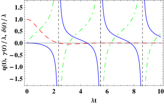
Figure 4: (Color online) Plot of $q$ (red dashed line), $\gamma$ (green dot-dashed line) and $\delta$ (blue continuous line) defined in Eq. (III.3), Eq. (IV.2) and Eq. (100) respectively, as functions of $\lambda t$ for the convolution of two equal exponential waiting time distributions. The vertical asymptotes denote the points where $q\left(t\right)$ goes through zero, so that $\gamma\left(t\right)$ diverges. The functions $\gamma\left(t\right)$ and $\delta\left(t\right)$ appear as time dependent coefficients in front of the various quantum channels in the time local quantum master equations given by Eq. (70) and Eq. (97), so that their sign determines P-divisibility and CP-divisibility of the corresponding quantum semi-Markov processes, as discussed in Sect. IV.1.

. In this case the region $\Omega_{+}$ can be exactly determined and is given by

$$\Omega_{+} = \bigcup_{n\in\mathbbm{N}}\left(\frac{1}{\lambda}\left(\pi+n\pi\right),\frac{1}{\lambda}\left(\frac{3}{4}\pi+n\pi\right)\right).$$ (85)

As already observed both measures become nonzero when $\left|q\left(t\right)\right|$ grows. The measure proposed by Breuer, Laine and Piilo according to Eq. (IV.2.2) can now be exactly calculated and is given by

$$\mathcal{N}\left(\Phi\right) = \sum^{\infty}_{n=0}\left(-\right)^{n+1}\left[q\left(\frac{\pi+n\pi}{\lambda}\right)-q\left(\frac{3\pi/4+n\pi}{\lambda}\right)\right]$$ (86)

$$= \frac{1}{e^{\pi}-1},$$

which is finite and independent on $\lambda$. It is to be stressed that considering the convolution of a higher number of exponential waiting time distributions one obtains a higher value for this measure, according to the fact that the overall waiting time distribution departs more and more from the memoryless exponential case Cox1965 (32). The measure proposed by Rivas, Huelga and Plenio instead is equal to infinity $\mathcal{I}\left(\Phi\right)\eqcirc\infty$, due to the fact that $q\left(t\right)$ goes through zero and therefore $\gamma\left(t\right)$ diverges. Actually $\mathcal{I}\left(\Phi\right)$ is equal to infinity whenever the inverse time evolution mapping fails to exist. It therefore quantifies in the same way non-Markovianity for quite different situations, e.g. in this case waiting time distributions given by the convolution of a different number of exponentials.

As a further example we consider a convolution of two different exponential distributions, corresponding to Eq. (48) and Eq. (51), so that one now has

$$\gamma\left(t\right) = 2\frac{p}{s}\frac{1}{1+\chi\operatorname{Coth}\left(\frac{st}{2}\chi\right)}.$$ (87)

Recalling Eq. (50) and Eq. (52) the argument of the hyperbolic cotangent is real, so that $\gamma\left(t\right)$ always stays positive, if $p\leqslant s^{2}/8$. In this case, despite the underlying non-Markovian classical process, both measures of non-Markovianity are equal to zero. The behavior of $q\left(t\right)$ and $\gamma\left(t\right)$ for this case is depicted in Fig. 5

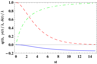
Figure 5: (Color online) The same as Fig. 4, but for the convolution of two different exponential waiting time distributions. We plot the quantities as a function of $st$, taking $p/s^{2}=0.12$. Note that in this case $\gamma\left(t\right)$ (green dot-dashed line) is always positive, while $\delta\left(t\right)$ (blue continuous line) is always negative. The function $q\left(t\right)$ (red dashed line) monotonically decreases reaching the value zero only at infinity.

. When $p>s^{2}/8$, which includes the case $\lambda_{1}=\lambda_{2}$, $q\left(t\right)$ again oscillates between positive and negative values, so that one has a similar behavior as before, with $\mathcal{N}\left(\Phi\right)$ assuming a finite value and $\mathcal{I}\left(\Phi\right)\eqcirc\infty$.

Finally let us consider a convex mixture of two memoryless distributions as given by Eq. (53), so that $q\left(t\right)$ is now given by Eq. (55) and one has

$$\gamma\left(t\right)=\langle\lambda\rangle\frac{1+\frac{1}{4}\frac{\left(\lambda_{1}+\lambda_{2}-3\langle\lambda\rangle\right)\left(\lambda_{1}+\lambda_{2}+\langle\lambda\rangle\right)-\overline{\lambda}^{2}}{\overline{\lambda}\langle\lambda\rangle}\operatorname{Coth}\left(\frac{\bar{\lambda}t}{2}\right)}{1+\frac{\left(\lambda_{1}+\lambda_{2}-3\langle\lambda\rangle\right)}{\overline{\lambda}}\operatorname{Coth}\left(\frac{\bar{\lambda}t}{2}\right)},$$ (88)

which according to the definitions of $\langle\lambda\rangle$ and $\overline{\lambda}$ given in Eq. (56) and Eq. (57) can be checked to always take on positive values. Its behavior is given in Fig. 6

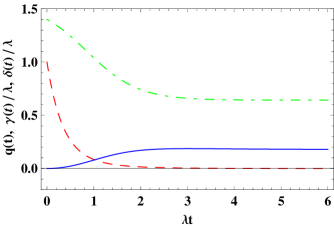
Figure 6: (Color online) The same as Fig. 4, but for a convex mixture of two different exponential waiting time distributions. We plot $q$ (red dashed line), $\gamma$ (green dot-dashed line) and $\delta$ (blue continuous line) as a function of $\lambda t$, taking $\lambda_{1}=a_{1}\lambda$ and $\lambda_{2}=a_{2}\lambda$, with $a_{1}=1$ and $a_{2}=6$, together with mixing parameter $\mu=0.6$. For this kind of waiting time distribution all functions always stay positive, quickly reaching an asymptotic constant value.

. In this situation both measures are equal to zero.

IV.3 Dephasing dynamics via projection

A quantum dynamics corresponding to pure dephasing is also obtained considering a CPT map $\mathcal{E}$ which is also a projection, that is

$$\mathcal{E}_{{}_{P}}\rho = \sigma_{+}\sigma_{-}\rho\sigma_{+}\sigma_{-}+\sigma_{-}\sigma_{+}\rho\sigma_{-}\sigma_{+}$$ (89)

so that one has idempotency $\mathcal{E}^{2}_{{}_{P}}=\mathcal{E}_{{}_{P}}$. For this case the analysis closely follows the one performed for $\mathcal{E}_{z}$, but the crucial quantity instead of $q\left(t\right)$ is the survival probability $g\left(t\right)$, similarly to the classical case with $\pi=1/2$ dealt with in Sect. III.1. The matrix $F$ is given by

$$F\left(t,0\right) = \operatorname{diag}\left(1,g\left(t\right),g\left(t\right),1\right)$$ (90)

and the time-local master equation reads

$$\frac{\mathrm{d}}{\operatorname{dt}}\rho\left(t\right) = h\left(t\right)\left(\mathcal{L}_{+-}\left[\rho\left(t\right)\right]+\mathcal{L}_{-+}\left[\rho\left(t\right)\right]\right),$$ (91)

with Lindblad operators

$$\mathcal{L}_{+-}\left[\rho\right] = \sigma_{+}\sigma_{-}\rho\sigma_{+}\sigma_{-}-\frac{1}{2}\left\{\sigma_{+}\sigma_{-},\rho\right\}$$ (92)

and similarly for $\mathcal{L}_{-+}$. The quantity $h\left(t\right)$ is given by

$$h\left(t\right) = \frac{f\left(t\right)}{g\left(t\right)}$$

$$= -\frac{\mathrm{d}}{\operatorname{dt}}\log g\left(t\right),$$

which provides the so called hazard rate function associated to the waiting time distribution $f\left(t\right)$, given by the ratio of waiting time distribution and survival probability. It gives information on the probability for the first jump to occur right after time $t$ Ross2007 (39). Note that the survival probability is a positive monotonously decreasing function, and the hazard rate function is always positive. As a result CP-divisibility always holds, so that both non-Markovianity measures are equal to zero, whatever the waiting time distribution is.

IV.4 Dissipative dynamics and time-local equation

The choice of CPT map considered above, corresponding to pure dephasing, shows how different probability densities for the waiting time, corresponding to different distributions of the action of the quantum operation in time, can lead to dynamics whose measures of non-Markovianity can be both positive or zero, irrespective of the fact that the only memoryless waiting time distribution is the exponential one. In this case, however, there is no direct connection to a classical dynamics, since only the coherences evolve in time. Another natural choice of CPT map which leads to a non trivial dynamics for the populations is given by

$$\mathcal{E}_{\pm}\rho = \sigma_{-}\rho\sigma_{+}+\sigma_{+}\rho\sigma_{-},$$ (94)

which satisfies $\mathcal{E}_{\pm}^{2n}=\mathcal{E}^{2}_{\pm}$ and $\mathcal{E}_{\pm}^{2n+1}=\mathcal{E}_{\pm}$, so that one can obtain the explicit representation

$$\rho_{11}\left(t\right) = p_{\operatorname{{even}}}\left(t\right)\rho_{11}(0)+p_{\operatorname{{odd}}}\left(t\right)\rho_{00}\left(0\right)$$

$$\rho_{10}\left(t\right) = g(t)\rho_{10}(0)$$

$$\rho_{01}\left(t\right) = g(t)\rho_{01}(0)$$

$$\rho_{00}\left(t\right) = p_{\operatorname{{odd}}}\left(t\right)\rho_{11}\left(0\right)+p_{\operatorname{{even}}}\left(t\right)\rho_{00}(0)$$ (95)

where $g(t)$ denotes as usual the survival probability. As in the previous case we can obtain the matrix $F$ representing the action of the map with respect to the chosen basis of operators in $\mathbbm{C}^{2}$, now given by

$$F\left(t,0\right) = \operatorname{diag}\left(1,g\left(t\right),g\left(t\right),q\left(t\right)\right)$$ (96)

and accordingly the time-convolutionless master equation reads

$$\frac{\mathrm{d}}{\operatorname{dt}}\rho\left(t\right)=\gamma\left(t\right)\left(\mathcal{L}_{+}\left[\rho\left(t\right)\right]+\mathcal{L}_{-}\left[\rho\left(t\right)\right]\right)+\delta\left(t\right)\mathcal{L}_{z}\left[\rho\left(t\right)\right],$$ (97)

where besides $\mathcal{L}_{z}$ as given by Eq. (71) the quantum channels

$$\mathcal{L}_{+}\left[\rho\right]=\sigma_{+}\rho\sigma_{-}-\frac{1}{2}\left\{\sigma_{-}\sigma_{+},\rho\right\}$$ (98)

and

$$\mathcal{L}_{-}\left[\rho\right] = \sigma_{-}\rho\sigma_{+}-\frac{1}{2}\left\{\sigma_{+}\sigma_{-},\rho\right\}$$ (99)

appear. The time dependent rate $\gamma\left(t\right)$ is still given by Eq. (IV.2), while the function $\delta\left(t\right)$ is given by the difference

$$\delta\left(t\right) = \frac{1}{2}\left(h\left(t\right)-\gamma\left(t\right)\right),$$ (100)

where $h\left(t\right)$ is the so called hazard rate function introduced in Eq. (IV.3), which is always positive.

IV.4.1 Divisibility

Also in this case we can consider the divisibility properties of the time evolution. According to the matrix representation of the map, Eq. (3) now leads to

$$F\left(t,s\right) = \operatorname{diag}\left(1,\frac{g\left(t\right)}{g\left(s\right)},\frac{g\left(t\right)}{g\left(s\right)},\frac{q\left(t\right)}{q\left(s\right)}\right),$$ (101)

so that thanks to the property of the survival probability the only condition for P-divisibility is still given by Eq. (74). Therefore the map is  P-divisible whenever $\left|q\left(t\right)\right|$ is a monotonic decreasing function. Note that this condition implies positivity of $\gamma\left(t\right)$, and therefore of the time dependent rate in front of the $\mathcal{L}_{+}$ and $\mathcal{L}_{-}$ channels, which affect the dynamics of the populations. In order to study CP-divisibility one has to consider the associated Choi matrix, whose positivity is granted upon the further condition

$$\frac{g\left(t\right)}{g\left(s\right)} \leqslant \frac{1}{2}\left(1+\frac{q\left(t\right)}{q\left(s\right)}\right),$$ (102)

which sets a non trivial requirement, implying positivity of the function $\delta\left(t\right)$ which provides the coefficient of the purely quantum channel $\mathcal{L}_{z}$. Thus CP-divisibility is violated if and only if at least one of the prefactors in the time-local form Eq. (97) becomes negative. Note however that in this case, due to the presence of different quantum channels, P-divisibility and CP-divisibility are not necessarily violated together, since it can well happen that $\gamma\left(t\right)$ stays positive, but $\delta\left(t\right)$ takes on negative values. As discussed in the examples below and shown in Fig. 5, for a suitable choice of waiting time distribution one can have a process which is P-divisible, but not CP-divisible.

IV.4.2 Measures of non-Markovianity

Also for this model we can obtain the explicit expression for the measures of non-Markovianity according to Breuer2009b (12) and Rivas2010a (13). The trace distance now reads

$$D\left(\rho^{1}\left(t\right),\rho^{2}\left(t\right)\right)=\sqrt{q^{2}\left(t\right)\Delta_{p}\left(0\right)^{2}+\left|\Delta_{c}\left(0\right)\right|^{2}g^{2}\left(t\right)},$$ (103)

where we have used the same notation as in Eq. (77) and Eq. (78), so that the derivative is

$$\sigma\left(t,\rho^{1,2}\left(0\right)\right)=\frac{\Delta_{p}\left(0\right)^{2}q\left(t\right)\dot{q}\left(t\right)-\left|\Delta_{c}\left(0\right)\right|^{2}g\left(t\right)f\left(t\right)}{\sqrt{q^{2}\left(t\right)\Delta_{p}\left(0\right)^{2}+\left|\Delta_{c}\left(0\right)\right|^{2}g^{2}\left(t\right)}}$$ (104)

and can grow in the region $\Omega_{+}$ where $q\left(t\right)$ and $\dot{q}\left(t\right)$ have the same sign. In this region $\left|q\left(t\right)\right|$ does increase. The growth is maximal for $\Delta_{c}\left(0\right)=0$ and $\Delta_{p}\left(0\right)=1$, so that the couple of states which maximize it is given by the projectors on ground and excited state. As a result, similarly as before we have for the measure of non-Markovianity introduced by Breuer, Laine and Piilo

$$\mathcal{N}\left(\Phi\right) = \int_{\Omega_{+}}\mathrm{d}t\frac{\mathrm{d}}{\mathrm{d}t}\left|q\left(t\right)\right|$$

$$= \sum_{i}\left(\left|q\left(b_{i}\right)\right|-\left|q\left(a_{i}\right)\right|\right).$$

This result for the choice of CPT map $\mathcal{E}_{\pm}$ is right the same as for the CPT map $\mathcal{E}_{z}$. This measure becomes nonzero if and only if P-divisibility is broken. It can be shown that this is generally the case for a bistochastic map $\Phi$ in $\mathbbm{C}^{2}$.

The criterion of Rivas, Huelga and Plenio instead assigns to the map a nonzero measure whenever one of the coefficients $\gamma\left(t\right)$ or $\delta\left(t\right)$ take on negative values, so that CP-divisibility is broken. Since $h\left(t\right)$ is always positive, these two functions can take on negative values only on separate time intervals, as can also be seen from Fig. 4. The measure is then given by Eq. (81), where according to Eq. (82) we have $\mathfrak{g}\left(t\right)=0$ whenever both $\gamma\left(t\right)$ and $\delta\left(t\right)$ are positive, while $\mathfrak{g}\left(t\right)=-2\gamma\left(t\right)$ whenever $\gamma\left(t\right)$ is negative, and $\mathfrak{g}\left(t\right)=-2\delta\left(t\right)$ in the complementary time intervals in which $\delta\left(t\right)$ takes on negative values. Note that this measure $\mathcal{I}\left(\Phi\right)$ can become positive even if the measure $\mathcal{N}\left(\Phi\right)$ is zero. Indeed the latter measure for this dynamics is related to P-divisibility rather than CP-divisibility.

IV.4.3 Population dynamics

For the dynamics described by Eq. (62), with the CPT map given by $\mathcal{E}_{\pm}$ as in Eq. (94), coherences and populations decouple, and the populations obey the same equation as the transition probabilities of the classical semi-Markov processes considered in Sect. III for $\pi=1$ and arbitrary waiting time distribution. This is immediately seen identifying the two components of the probability vector with the populations in excited and ground state. Setting $P_{+}\left(t\right)=\langle+|\rho\left(t\right)|+\rangle$ and $P_{-}\left(t\right)=\langle-\rho\left(t\right)|-\rangle$ one has in fact from Eq. (62) with $\mathcal{E}_{\pm}$ the integrodifferential rate equations

$$\frac{\mathrm{d}}{\operatorname{dt}}P_{\pm}\left(t\right) = \int^{t}_{0}d\tau k\left(t-\tau\right)\left[P_{\mp}\left(\tau\right)-P_{\pm}\left(\tau\right)\right]$$ (106)

corresponding to Eq. (17) for

$$W\left(\tau\right) = \left(\begin{array}[]{cc}-1&1\\ 1&-1\end{array}\right)k\left(\tau\right).$$ (109)

Also in the classical case the integrodifferential time evolution equation can be generally recast in time local form Hanggi1978a (40). In this case Eq. (106) would then simply correspond to the diagonal matrix elements of Eq. (97).

The Kolmogorov distance as in Eq. (61) is given by

$$D_{K}\left(\left\{P_{+}^{1}\left(t\right),P_{-}^{1}\left(t\right)\right\},\left\{P_{+}^{2}\left(t\right),P_{-}^{2}\left(t\right)\right\}\right) = \left|\Delta_{p}\left(0\right)\right|\left|q\left(t\right)\right|,$$

so that $\mathcal{N}\left(\Phi\right)$, being obtained by considering as initial states the projections onto ground and excited state, is also given by taking the maximum over the possible initial classical states of the integral of the derivative $\sigma_{K}$ of the Kolmogorov distance in the time intervals in which it is positive. Growth of the Kolmogorov distance again depends on the behavior of $\left|q\left(t\right)\right|$ only, which determines whether the map is P-divisible or not. In view of this connection it appears that one can have non-Markovianity measure $\mathcal{N}\left(\Phi\right)$ for the quantum map $\Phi$ equal to zero even if the dynamics for the populations can be related to a non-Markovian classical process. Again this is not too surprising, since the one-point probabilities cannot really keep track of Markovianity or non-Markovianity in the classical sense, even though in the non-Markovian case they can show up different behaviors than those typical of the Markovian one.

IV.4.4 Explicit examples

At variance with the case of pure dephasing, the two measures of non-Markovianity do not agree for this model. The measure $\mathcal{N}\left(\Phi\right)$ becomes positive as soon as P-divisibility is broken, which depends on the sign of $\gamma\left(t\right)$ only, while $\mathcal{I}\left(\Phi\right)$ becomes positive even when only CP-divisibility does not hold, which also depends on the sign of the function $\delta\left(t\right)$ appearing in front of the purely quantum channel $\mathcal{L}_{z}$, which determines the dynamics of the coherences. To consider the behavior of the measures for this model we thus have to consider also the quantity $\delta\left(t\right)$, which is simply equal to zero for an exponential waiting time distribution, so that in the proper Markovian case this pure quantum channel is not available.

For the case of the convolution of two equal exponential distributions exploiting Eq. (40) and  Eq. (41) together with Eq. (84) we have

$$\delta\left(t\right) = \frac{\lambda}{2}\left(\frac{\lambda t}{1+\lambda t}-\frac{1}{1+\operatorname{cotg}\left(\lambda t\right)}\right),$$ (110)

so that both $\gamma\left(t\right)$ and $\delta\left(t\right)$ oscillate in sign and diverge when $\operatorname{cotg}\left(\lambda t\right)$ takes on the value minus one, as shown in Fig. 4. In this case both measures are positive, while considering the convolution of two different exponential distributions one has thanks to Eq. (48), Eq. (49) and Eq. (87)

$$\delta\left(t\right) = \frac{p}{s}\left(\frac{1}{1+\xi\operatorname{Coth}\left(\frac{st}{2}\xi\right)}-\frac{1}{1+\chi\operatorname{Coth}\left(\frac{st}{2}\chi\right)}\right).$$ (111)

If the ratio $\lambda_{1}/\lambda_{2}$ is far enough from one $\gamma\left(t\right)$ given by Eq. (87) as discussed above stays always positive, so that one has P-divisibility and the measure $\mathcal{N}\left(\Phi\right)$ is equal to zero. On the contrary the function $\delta\left(t\right)$ is negative, so that the coefficient in front of the quantum channel is always negative and CP-divisibility is violated , thus determining a positive measure $\mathcal{I}\left(\Phi\right)$. This situation is considered in Fig. 5.

As a last example we consider a convex mixture of exponential distributions, leading to Eq. (88) as well as

$$h\left(t\right) = \frac{\mu\lambda_{1}\mathrm{e}^{-\lambda_{1}t}+\left(1-\mu\right)\lambda_{2}\mathrm{e}^{-\lambda_{2}t}}{\mu\mathrm{e}^{-\lambda_{1}t}+\left(1-\mu\right)\mathrm{e}^{-\lambda_{2}t}}.$$ (112)

For this case, independently of the value of the mixing parameter $\mu$, one has that both $\gamma\left(t\right)$ and $\delta\left(t\right)$ stay positive. A dynamics of this kind for an open quantum system is often termed time-dependent Markovian Laine2010a (16), since at any time the generator is in Lindblad form. Once again both measures $\mathcal{N}\left(\Phi\right)$ and $\mathcal{I}\left(\Phi\right)$ give a zero value of non-Markovianity, despite the fact that the underlying waiting time distribution is not memoryless, corresponding to a population dynamics described by a classical semi-Markov process which is not Markovian.

V Conclusions and outlook

In this paper we have analyzed the notion of non-Markovianity for the dynamics of open quantum systems, starting from the classical setting and focusing on concrete examples. While knowledge of a non-Markovian classical process requires information on all the conditional probability densities, when studying the dynamics of an open system one only considers the evolution of the state, expressed by a probability vector in the classical case and a statistical operator for a quantum system. The notion of non-Markovianity for classical processes and for dynamical evolutions are therefore by necessity distinct concepts. One is then naturally lead to the question whether and how the non-Markovianity of a process reflects itself in the behavior of the one-point probability. It turns out that the notion of P-divisibility, in the sense of the existence of well-defined stochastic matrices connecting probability vectors at different time points, as well as monotonic decrease in time of the Kolmogorov distance among states arising from different initial conditions, are typical features of Markovian processes in the classical case. The lack of these properties can thus be interpreted as signature of non-Markovianity, and used to quantify it. Note that due to the fact that the classical definition of non-Markovianity actually involves all $n$-point probability densities, these signatures as expected indeed provide a different notion of non-Markovianity, which only gives a sufficient condition in order to assess non-Markovianity in the original sense. This behavior is shown by means of example relying on the study of certain semi-Markov processes.

Such signatures of non-Markovianity can be brought over to the quantum framework, considering the notion of CP-divisibility, corresponding to the fact that the quantum time evolution map can be arbitrary split into CPT maps corresponding to intermediate time intervals, and of the trace distance, which is the quantum version of the Kolmogorov distance. These two criteria are at the basis of two recently introduced measures of non-Markovianity for open quantum systems Breuer2009b (12, 13), which we here compare considering a quantum counterpart of classical semi-Markov processes. Moreover, analyzing both the integrodifferential and the time local form of the equations of motion, we show that one can point to possible signatures of non-Markovianity to be read directly at the level of the equation, despite the fact that Markovianity or non-Markovianity itself is a feature of the solution. In this respect it appears that the time local form of the equations, despite isolated singularities, is certainly more convenient.

More specifically, the classes of examples discussed in the paper, besides clarifying the relationship between the distinct notions of non-Markovianity used for classical processes and for dynamical evolutions, allow an exact evaluation of the measure of non-Markovianity introduced for quantum dynamical maps, see e.g. the remarkable result given by Eq. (86). These physical examples further allow an explicit comparison of the two measures for whole classes of quantum dynamical maps. In particular, as shown by Eq. (IV.2.2) and Eq. (IV.2.2) and discussed thoroughly in Sect. IV.2.3, we put into evidence that the measure based on CP-divisibility Rivas2010a (13) gives the same infinite value to quite different time evolutions, at variance with the measure based on the dynamics of the trace distance Breuer2009b (12), which assigns to them different weights.

In this paper we have discussed the different definitions of non-Markovianity relevant for classical stochastic processes and dynamical evolutions. The latter are based on the divisibility of the time evolution map and on the dynamic behavior of the distinguishability among different initial states. While these definitions of non-Markovianity can be considered both in the classical and the quantum case, as discussed in Sect. III and Sect. IV the original definition of non-Markovianity for a classical process cannot be transferred as such to the quantum realm, because of basic principles of quantum mechanics. On the one hand to make statements about the value of a certain observables at different times, a measurement scheme has to be specified, which affects the subsequent time evolution; on the other hand the statistical operator of a quantum systems provide different, and generally incompatible, classical probability densities for different observables, as a typical feature of quantum probability with respect to classical probability Holevo2001 (41, 42). In this respect one should be satisfied with different definitions and measures of non-Markovianity within the classical and the quantum framework.

It is clear that physical systems can provide us with much more complicated dynamics than the one considered in this paper and the recent literature. However the analysis of these situations sheds light on the basic ideas used in defining Markovianity or non-Markovianity of a time evolution, and to their connection with the classical definition of non-Markovian, thus possibly opening the way for a more refined and general analysis.

VI Acknowledgments

BV and AS gratefully acknowledge financial support by MIUR under PRIN2008, EML by the Graduate School of Modern Optics and Photonics, JP by the Magnus Ehrnrooth Foundation, and HPB by the German Academic Exchange Service.

References

- (1) H.-P. Breuer and F. Petruccione, The Theory of Open Quantum Systems (Oxford University Press, Oxford, 2002)
- (2) J. T. Stockburger and H. Grabert, Phys. Rev. Lett. 88, 170407 (2002)
- (3) S. Daffer, K. Wódkiewicz, J. D. Cresser, and J. K. McIver, Phys. Rev. A 70, 010304 (2004)
- (4) J. Piilo, S. Maniscalco, K. Härkönen, and K.-A. Suominen, Phys. Rev. Lett. 100, 180402 (2008)
- (5) H.-P. Breuer and B. Vacchini, Phys. Rev. Lett. 101, 140402 (2008)
- (6) A. Shabani and D. A. Lidar, Phys. Rev. Lett. 102, 100402 (2009)
- (7) D. Chruscinski and A. Kossakowski, Phys. Rev. Lett. 104, 070406 (2010)
- (8) A. Barchielli, C. Pellegrini, and F. Petruccione, EPL 91, 24001 (2010)
- (9) E.-M. Laine, J. Piilo, and H.-P. Breuer, EPL 92, 60010 (2010)
- (10) A. A. Budini, Phys. Rev. A 69, 042107 (2004)
- (11) M. M. Wolf, J. Eisert, T. S. Cubitt, and J. I. Cirac, Phys. Rev. Lett. 101, 150402 (2008)
- (12) H.-P. Breuer, E.-M. Laine, and J. Piilo, Phys. Rev. Lett. 103, 210401 (2009)
- (13) A. Rivas, S. F. Huelga, and M. B. Plenio, Phys. Rev. Lett. 105, 050403 (2010)
- (14) G. Lindblad, Comm. Math. Phys. 48, 119 (1976)
- (15) V. Gorini, A. Kossakowski, and E. C. G. Sudarshan, J. Math. Phys. 17, 821 (1976)
- (16) E.-M. Laine, J. Piilo, and H.-P. Breuer, Phys. Rev. A 81, 062115 (2010)
- (17) M. Hayashi, Quantum Information (Springer-Verlag, Berlin, 2006)
- (18) M. M. Wolf and J. I. Cirac, Commun. Math. Phys. 279, 147 (2008)
- (19) J. R. Norris, Markov Chains (Cambridge University Press, Cambridge, 1999)
- (20) D. Chruscinski, A. Kossakowski, P. Aniello, G. Marmo, and F. Ventriglia, Open Syst. Inf. Dyn. 17, 255 (2010)
- (21) D. Chruscinski and A. Kossakowski, e-print arXiv:1010:4745v1 (2010)
- (22) D. Chruscinski, A. Kossakowski, and A. Rivas, e-print arXiv:1102:4318v1 (2011)
- (23) A. Rivas and S. F. Huelga, e-print arXiv:1104:5242v1 (2011)
- (24) V. Karimipour and L. Memarzadeh, e-print arXiv:1105:2728v1 (2011)
- (25) N. van Kampen, Braz. J. Phys. 28, 90 (1998)
- (26) D. T. Gillespie, Am. J. Phys. 66, 533 (1998)
- (27) P. Hänggi and H. Thomas, Z. Phys. B 26, 85 (1977)
- (28) P. Hänggi and H. Thomas, Phys. Rep. 88, 207 (1982)
- (29) W. Feller, An introduction to probability theory and its applications. Vol. II (John Wiley & Sons Inc., New York, 1971)
- (30) W. Feller, Proc. Nat. Acad. Sci. U.S.A. 51, 653 (1964)
- (31) D. R. Cox and H. D. Miller, The theory of stochastic processes (John Wiley & Sons Inc., New York, 1965)
- (32) J. Medhi, Stochastic Processes (John Wiley & Sons, 1994)
- (33) C. A. Fuchs and J. van de Graaf, IEEE Trans. Inf. Th. 45, 1216 (1999)
- (34) M. Nielsen and I. Chuang, Quantum Computation and Quantum Information (Cambridge University Press, Cambridge, 2000)
- (35) H.-P. Breuer and B. Vacchini, Phys. Rev. E 79, 041147 (2009)
- (36) A. Smirne and B. Vacchini, Phys. Rev. A 82, 022110 (2010)
- (37) M. D. Choi, Lin. Alg. Appl. 10, 285 (1975)
- (38) P. Haikka, J. D. Cresser, and S. Maniscalco, Phys. Rev. A 83, 012112 (2011)
- (39) S. M. Ross, Introduction to probability models (Academic Press, Burlington, MA, 2007)
- (40) P. Hänggi, H. Thomas, H. Grabert, and P. Talkner, J. Stat. Phys. 18, 155 (1978)
- (41) A. S. Holevo, Statistical Structure of Quantum Theory, Vol. m 67 of Lecture Notes in Physics (Springer, Berlin, 2001)
- (42) F. Strocchi, An introduction to the mathematical structure of quantum mechanics (World Scientific, 2005)