Robustness of quantum discord to sudden death in NMR

Abstract

We investigate the dynamics of entanglement and quantum discord of two qubits in liquid state homonuclear NMR. Applying a phenomenological description for NMR under relaxation process, and taking a group of typical parameters of NMR, we show that when a zero initial state $|00\rangle$ experiences a relaxation process, its entanglement disappears completely after a sequence of so-called sudden deaths and revivals, while the quantum discord retains remarkable values after a sequence of oscillations. That is to say, the quantum discord is more robust than entanglement.

1 Introduction

Entanglement is one of the most striking features for our deeper understanding of the quantum world, and is widely seen as the main resource for quantum information processing [1, 2]. However, entanglement is not the only type of useful correlation. It has been found that entanglement is not necessary for deterministic quantum computation with one pure qubit (DQC1) [3, 4, 5], but another quantum correlation, introduced by [6, 7], called quantum discord (QD), is responsible for the computational efficiency of DQC1. Besides, QD has also been used for some studies such as quantum phase transition [8] and the process of Grover search[9]. Recently, the dynamics of QD has attracted more attentions, such as the robustness of QD to sudden death [10], QD in Heisenberg models [11] and Non-Markovian effect of QD [12].

Nuclear magnetic resonance (NMR) has been used to demonstrate basic concepts of quantum information processing, and has been leading the field both in terms of number of qubits and control techniques [13, 14]. The studies of dynamics characteristics and the implementations for quantum information processing of NMR systems have also received a great deal of attentions in recent years [15, 16, 17, 18, 19, 20].

Due to the fundamental and practical significance, we wish to investigate the dynamics behaviors of entanglement and QD of two qubits in NMR systems. The rest of this paper is organized as follows. In Sec.2, we present a brief review of the entanglement, QD and liquid state two qubits NMR systems. In Sec.3, we investigate the dynamics of entanglement and quantum discord of two qubits NMR without relaxation. In Sec.4, applying a phenomenological method, we investigate the dynamics of entanglement and quantum discord of two qubits NMR with relaxation. Sec.5 is a brief summary.

2 Entanglement,quantum discord, NMR systems

We first recall some basics about entanglement, QD and NMR.

2.1 Concurrence of two qubits states

Two quantum systems A and B, described by the Hilbert spaces $H^{A}$ and $H^{B}$, and the composite system AB is described by the Hilbert space $H^{A}$ $\otimes$ $H^{B}$. A state $\rho$ on $H^{A}$ $\otimes$ $H^{B}$ is called a separable state if and only if it can be written as the form

$$\rho=\sum_{i=1}^{n}p_{i}\rho_{i}^{A}\otimes\rho_{i}^{B},$$ (1)

where n is a positive integer, $p_{i}\geq 0$, $\sum_{i=1}^{n}p_{i}=1$, $\{\rho_{i}^{A}\}_{i=1}^{n}$ are density operators on $H^{A}$, $\{\rho_{i}^{B}\}_{i=1}^{n}$ are density operators on $H^{B}$. A state is called an entangled state if it is not a separable state. For two qubits, one of the most widely used entanglement measures is the so-called concurrence, we will use it as the quantifier in this paper. For two qubits state $\rho$, the concurrence of $\rho$ is defined as [21]

$$C(\rho)=\max\{0,\lambda_{1}-\lambda_{2}-\lambda_{3}-\lambda_{4}\},$$ (2)

where $\lambda_{1}$, $\lambda_{2}$, $\lambda_{3}$, $\lambda_{4}$ are the square roots of the eigenvalues of the matrix $\rho\widetilde{\rho}$ in decreasing order, and

$$\widetilde{\rho}=(\sigma_{y}\otimes\sigma_{y})\rho^{*}(\sigma_{y}\otimes\sigma_{y}),$$ (3)

$\sigma_{y}$ is the Pauli matrix, $\rho^{*}$ is the complex conjugate of $\rho$. For convenience, in Eq.(2) we denote

$$\overline{C}(\rho)=\lambda_{1}-\lambda_{2}-\lambda_{3}-\lambda_{4},$$ (4)

and call it pseudo-concurrence.

2.2 Quantum discord of two qubits states

The quantum discord of $\rho$ on $H^{A}$ $\otimes$ $H^{B}$ (with respect to system A) is defined as [6, 7]

$$D_{A}(\rho)=S(\rho^{A})-S(\rho^{AB})+\inf_{\{|\alpha\rangle\langle\alpha|\otimes I\}_{\alpha=1}^{n_{A}}}\sum_{\alpha=1}^{n_{A}}p_{\alpha}S(\rho_{\alpha}^{B}).$$ (5)

In Eq.(5), $S(\cdot)$ is the entropy function, that is, e.g., $S(\rho^{A})=-tr_{A}(\rho^{A}\log_{2}\rho^{A})$. $n_{A}=dimH^{A}$, inf takes all projective measurements $\{|\alpha\rangle\langle\alpha|\otimes I\}_{\alpha=1}^{n_{A}}$ on system A, that is, $\{|\alpha\rangle\}_{\alpha=1}^{n_{A}}$ is an arbitrary orthonormal basis for $H^{A}$. We use $I$ to denote the identity operators on $H^{A}$ or on $H^{B}$. $p_{\alpha}=tr_{A}(|\alpha\rangle\langle\alpha|\otimes I\rho|\alpha\rangle\langle\alpha|\otimes I)$, $\rho_{\alpha}^{B}=|\alpha\rangle\langle\alpha|\otimes I\rho|\alpha\rangle\langle\alpha|\otimes I/p_{\alpha}$.

Quantum discord captures more correlation than entanglement, this can been seen by Eq.(1) and the fact that [6]

$$D_{A}(\rho)=0\Longleftrightarrow\rho=\sum_{\alpha=1}^{n_{A}}p_{\alpha}|\alpha\rangle\langle\alpha|\otimes\rho_{\alpha}^{B},$$ (6)

where, $\{|\alpha\rangle\}_{\alpha=1}^{n_{A}}$ is an arbitrary orthonormal basis for $H^{A}$, $\{\rho_{\alpha}^{B}\}_{\alpha=1}^{n_{A}}$ are density operators on $H^{B}$, $p_{\alpha}\geq 0$, $\sum_{\alpha=1}^{n_{A}}p_{\alpha}=1$. A state $\rho$ satisfying $D_{A}(\rho)=0$ is called zero quantum discord state or classical state. Comparing Eq.(1) with Eq.(6), it is obvious that a classical state must be a separable state.

Eq.(5) is difficult to optimize, even for two qubits states, up to now only few special states were found to allow analytical solutions [22, 23]. A technical definition of quantum discord, called geometrical measure, was introduced as [24],

$$D_{A}^{G}(\rho)=\inf_{\sigma}tr[(\rho-\sigma)^{2}],$$ (7)

where inf takes all $\sigma$ that $D_{A}(\sigma)=0$. Evidently,

$$D_{A}(\rho)=0\Longleftrightarrow D_{A}^{G}(\rho)=0.$$ (8)

One of the most elegant results about the definition of $D_{A}^{G}(\rho)$ is that it allows analytical expressions for all two qubits states. More specifically, for any two qubits state $\rho$ which can be written as

$$\rho=\frac{1}{4}(I\otimes I+\sum_{i=1}^{3}x_{i}\sigma_{i}\otimes I+\sum_{j=1}^{3}y_{j}I\otimes\sigma_{j}+\sum_{i,j=1}^{3}T_{ij}\sigma_{i}\otimes\sigma_{j}),$$ (9)

then [24],

$$D_{A}^{G}(\rho)=\frac{1}{4}(\sum_{i=1}^{3}x_{i}^{2}+\sum_{i,j=1}^{3}T_{ij}^{2}-\lambda_{\max}).$$ (10)

Where, $\sigma_{1}=\sigma_{x}$, $\sigma_{2}=\sigma_{y}$, $\sigma_{3}=\sigma_{z}$, are Pauli matrices, $\{x_{i}\}_{i=1}^{3}$, $\{y_{j}\}_{j=1}^{3}$, $\{T_{ij}\}_{i,j=1}^{3}$ are all real number sets. $\lambda_{\max}$ is the largest eigenvalue of the matrix $xx^{t}+TT^{t}$, $x=(x_{1},x_{2},x_{3})^{t}$, $T$ is the matrix $(T_{ij})$, t means transpose. Also

$$x_{i}=tr[\rho\sigma_{i}\otimes I],y_{j}=tr[\rho I\otimes\sigma_{j}],T_{ij}=tr[\rho\sigma_{i}\otimes\sigma_{j}].$$ (11)

(The explicit expressions for $\{x_{i}\}_{i=1}^{3}$ and $\{T_{ij}\}_{i,j=1}^{3}$ by the elements of $\rho$, see Appendix A.)

2.3 Two qubits in liquid state NMR

The Hamiltonian of two qubits in NMR (we focus on the liquid state NMR) is well described by [13]

$$\ \ H(t)=H_{sys}+H_{rf}(t),$$ (12)

$$\ \ H_{sys}=-\frac{\hbar\omega_{1}}{2}\sigma_{z}\otimes I-\frac{\hbar\omega_{2}}{2}I\otimes\sigma_{z}+\hbar J\sigma_{z}\otimes\sigma_{z},$$ (13)

$$H_{rf}(t)=-\frac{\hbar g_{1}}{2}[\cos(\omega t)\sigma_{x}\otimes I-\sin(\omega t)\sigma_{y}\otimes I]-\frac{\hbar g_{2}}{2}[\cos(\omega t)I\otimes\sigma_{x}-\sin(\omega t)I\otimes\sigma_{y}].$$ (14)

In $H_{sys}$, $\omega_{1}=B_{0}\gamma_{1}$, $\omega_{2}=B_{0}\gamma_{2}$, are called Lamor frequencies of two qubits (two nuclei), containing the chemical shifts. $B_{0}$ is the static magnetic field along z direction, $\gamma_{1}$, $\gamma_{2}$ are gyromagnetic ratios of two qubits. Typical values of $\omega_{1}$, $\omega_{1}$ are a few $10^{8}$Hz, and chemical shifts of a few $10^{3}$Hz to a few $10^{4}$Hz. J describes the spin-spin couplings including direct dipole-dipole coupling and indirect through-bond coupling. Spin-spin couplings are very small in NMR compared with the Lamor frequencies, for instance, a few $10^{2}$Hz.

In $H_{rf}(t)$, $g_{1}=B_{1}\gamma_{1}$, $g_{2}=B_{1}\gamma_{2}$, $B_{1}$ is the applied magnetic field rotating in x-y plane at frequency $\omega$, at or near the Lamor frequencies $\omega_{1}$, $\omega_{2}$. Typical values of $g_{1}$, $g_{2}$ are up to $10^{5}$Hz.

3 Dynamics of entanglement and quantum discord of two qubits in NMR without relaxation

We study the dynamics of two qubits NMR without relaxation. When the evolution time is much shorter than the relaxation time scales, the system can be approximated as an isolated system, and it evolves obeying the Schr$\ddot{o}$dinger equation

$$i\hbar\frac{\partial}{\partial t}|\Psi(t)\rangle=H(t)|\Psi(t)\rangle.$$ (15)

Notice that $H_{rf}(t)$ in Eq.(14) is time dependent, in order to cancel the time t in Hamiltonian $H(t)$, we put

$$|\Psi(t)\rangle=\exp[\frac{i\omega t}{2}(\sigma_{z}\otimes I+I\otimes\sigma_{z})]|\varphi(t)\rangle.$$ (16)

This transformation is widely used in NMR theory, sometimes called the method of rotating frame. With this transformation, we get

$$\ \ i\hbar\frac{\partial}{\partial t}|\varphi(t)\rangle=\widetilde{H}|\varphi(t)\rangle,$$ (17)

$$\widetilde{H}=-\frac{\hbar(\omega_{1}-\omega)}{2}\sigma_{z}\otimes I-\frac{\hbar(\omega_{2}-\omega)}{2}I\otimes\sigma_{z}+\hbar J\sigma_{z}\otimes\sigma_{z}-\frac{\hbar g_{1}}{2}\sigma_{x}\otimes I-\frac{\hbar g_{2}}{2}I\otimes\sigma_{x},$$ (18)

$$\ \ |\Psi(0)\rangle=|\varphi(0)\rangle.$$ (19)

In above reductions, we have used the facts that for any real number $\lambda$,

$$\ \ \ \ \ \ \ \ \ \ \ \ exp(i\lambda\sigma_{i})=\cos(\lambda)I+i\sin(\lambda)\sigma_{i},$$ (20)

$$exp(-i\lambda\sigma_{z})\sigma_{x}exp(i\lambda\sigma_{z})=\cos(2\lambda)\sigma_{x}+\sin(2\lambda)\sigma_{y},$$ (21)

$$exp(-i\lambda\sigma_{z})\sigma_{y}exp(i\lambda\sigma_{z})=\cos(2\lambda)\sigma_{y}-\sin(2\lambda)\sigma_{x}.$$ (22)

Since $\widetilde{H}$ is time independent, together with Eq.(16) and Eq.(19), we get

$$|\varphi(t)\rangle=\exp(\frac{t}{i\hbar}\widetilde{H})|\varphi(0)\rangle,$$ (23)

$$|\psi(t)\rangle=U(t)|\psi(0)\rangle,$$ (24)

$$U(t)=\exp[\frac{i\omega t}{2}(\sigma_{z}\otimes I+I\otimes\sigma_{z})]\exp(\frac{t}{i\hbar}\widetilde{H}).$$ (25)

In matrix notation,

$$\exp[\frac{i\omega t}{2}(\sigma_{z}\otimes I+I\otimes\sigma_{z})]=\left(\begin{array}[]{llll}e^{i\omega t}&0&0&0\\ 0&1&0&0\\ 0&0&1&0\\ 0&0&0&e^{-i\omega t}\end{array}\right),$$ (30)

$$\widetilde{H}=-\hbar\left(\begin{array}[]{llll}\frac{\omega_{1}+\omega_{2}}{2}-\omega-J&\frac{g_{2}}{2}&\frac{g_{1}}{2}&0\\ \frac{g_{2}}{2}&\frac{\omega_{1}-\omega_{2}}{2}+J&0&\frac{g_{1}}{2}\\ \frac{g_{1}}{2}&0&-\frac{\omega_{1}-\omega_{2}}{2}+J&\frac{g_{2}}{2}\\ 0&\frac{g_{1}}{2}&\frac{g_{2}}{2}&-\frac{\omega_{1}+\omega_{2}}{2}+\omega-J\end{array}\right).$$ (35)

Suppose the initial state is $|00\rangle$, that is

$$\rho=\left(\begin{array}[]{llll}1&0&0&0\\ 0&0&0&0\\ 0&0&0&0\\ 0&0&0&0\end{array}\right)$$ (40)

then

$$C(\rho)=0,\ \ \ \ \ \ D_{A}^{G}(\rho)=0.$$ (41)

After time t, $\rho$ will evolve to $\rho(t)$ as

$$\rho(t)=U(t)\rho U^{\dagger}(t),$$ (42)

where $\dagger$ means Hermitian conjugate. Then $C(\rho(t))$, $D_{A}^{G}(\rho(t))$ can be calculated by Eq.(2) and Eq.(10).

Fig.1 shows $\overline{C}(\rho(t))$ and $D_{A}^{G}(\rho(t))$ at $t=10^{-5}s$, $t=10^{-3}s$, $t=10^{-1}s$. Where we take the parameters of NMR as $\frac{\omega_{1}+\omega_{2}}{2}=3\times 10^{8}Hz$, $\frac{\omega_{1}-\omega_{2}}{2}=10^{4}Hz$, $J=3\times 10^{2}Hz$, $\frac{g_{1}}{2}=5\times 10^{4}Hz$, $\frac{g_{2}}{2}=5\times 10^{4}Hz$. From Fig.1 we see that, only near the frequency $\frac{\omega_{1}+\omega_{2}}{2}=3\times 10^{8}Hz$, entanglement and quantum discord are remarkably generated and evolved. It is a common phenomenon in NMR that the applied magnetic $B_{1}$ can effectively influence or control the nuclear spins at or near the resonance frequencies.

Fig.2 shows $\overline{C}(\rho(t))$ and $D_{A}^{G}(\rho(t))$ at the frequency $\frac{\omega_{1}+\omega_{2}}{2}=3\times 10^{8}Hz$, and we take the parameters of NMR as in Fig.1. From Fig.1 and Fig.2 we see that the dynamical behaviors of entanglement and quantum discord are similar in the evolution where we ignore the relaxation.

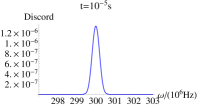
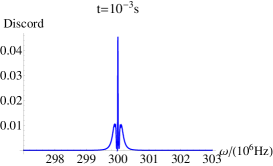
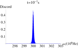
Figure 1: Pseudo-concurrence and quantum discord at time $t=10^{-5}s$, $t=10^{-3}s$, $t=10^{-1}s$.

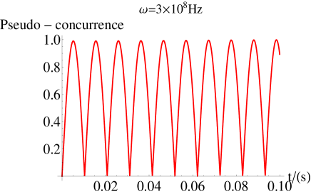
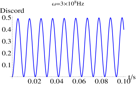
Figure 2: Pseudo-concurrence and quantum discord at frequency $\omega=\frac{\omega_{1}+\omega_{2}}{2}=3\times 10^{8}Hz$.

4 Dynamics of entanglement and quantum discord of two qubits in NMR with relaxation.

When the evolution time gets comparable to the relaxation time scales, the relaxation effects must be taken into account. The relaxation process in NMR can be described in a phenomenological way ([25];[14], 2.10)

$$\frac{d}{dt}\rho(t)=\frac{1}{i\hbar}[H(t),\rho(t)]-R,$$ (43)

$$\ \ \ \ R_{ij}=\frac{\rho_{ij}(t)-\rho_{ij}}{T_{ij}},$$ (44)

$$\ \ \ \ T_{ij}=\delta_{ij}T_{1}+(1-\delta_{ij})T_{2}.$$ (45)

Where $T_{1}$ is the energy relaxation rate, $T_{2}$ is the phase randomization rate. Theoretical calculations and experimental measurements for $T_{1}$ and $T_{2}$ are well developed. The typical value of $T_{1}$ is tens of seconds, and $T_{2}$ is easily on the order of 1 second or more.

Similar to Eq.(16), we let

$$\rho(t)=\exp[\frac{i\omega t}{2}(\sigma_{z}\otimes I+I\otimes\sigma_{z})]\sigma(t)\exp[-\frac{i\omega t}{2}(\sigma_{z}\otimes I+I\otimes\sigma_{z})],$$ (46)

notice that

$$\rho(0)=\sigma(0).$$ (47)

Using Eqs.(20-22), after some straightforward calculations, then Eq.(31) becomes

$$\frac{d\sigma(t)}{dt}=\frac{1}{i\hbar}[\widetilde{H},\sigma(t)]-\left(\begin{array}[]{llll}\frac{\sigma_{11}(t)}{T_{1}}&\frac{\sigma_{12}(t)}{T_{2}}&\frac{\sigma_{13}(t)}{T_{2}}&\frac{\sigma_{14}(t)}{T_{2}}\\ \frac{\sigma_{21}(t)}{T_{2}}&\frac{\sigma_{22}(t)}{T_{1}}&\frac{\sigma_{23}(t)}{T_{2}}&\frac{\sigma_{24}(t)}{T_{2}}\\ \frac{\sigma_{31}(t)}{T_{2}}&\frac{\sigma_{32}(t)}{T_{2}}&\frac{\sigma_{33}(t)}{T_{1}}&\frac{\sigma_{34}(t)}{T_{2}}\\ \frac{\sigma_{41}(t)}{T_{2}}&\frac{\sigma_{42}(t)}{T_{2}}&\frac{\sigma_{43}(t)}{T_{2}}&\frac{\sigma_{44}(t)}{T_{1}}\end{array}\right)+\left(\begin{array}[]{llll}\frac{\sigma_{11}(0)}{T_{1}}&\frac{\sigma_{12}(0)}{T_{2}}e^{-i\omega t}&\frac{\sigma_{13}(0)}{T_{2}}e^{-i\omega t}&\frac{\sigma_{14}(0)}{T_{2}}e^{-2i\omega t}\\ \frac{\sigma_{21}(0)}{T_{2}}e^{i\omega t}&\frac{\sigma_{22}(0)}{T_{1}}&\frac{\sigma_{23}(0)}{T_{2}}&\frac{\sigma_{24}(0)}{T_{2}}e^{-i\omega t}\\ \frac{\sigma_{31}(0)}{T_{2}}e^{i\omega t}&\frac{\sigma_{32}(0)}{T_{2}}&\frac{\sigma_{33}(0)}{T_{1}}&\frac{\sigma_{34}(0)}{T_{2}}e^{-i\omega t}\\ \frac{\sigma_{41}(0)}{T_{2}}e^{2i\omega t}&\frac{\sigma_{42}(0)}{T_{2}}e^{i\omega t}&\frac{\sigma_{43}(0)}{T_{2}}e^{i\omega t}&\frac{\sigma_{44}(0)}{T_{1}}\end{array}\right)$$ (56)

Eq.(36) is a first-order linear nonhomogeneous ordinary differential equations with constant coefficients in the functions $\sigma_{11}(t),\sigma_{12}(t),\sigma_{13}(t),\sigma_{14}(t),\sigma_{21}(t),...,\sigma_{44}(t)$. If we denote $\sigma(t)$ and the last matrix in Eq.(36) by

$$\overrightarrow{\sigma}(t)=(\sigma_{11}(t),\sigma_{12}(t),\sigma_{13}(t),\sigma_{14}(t),\sigma_{21}(t),...,\sigma_{44}(t))^{t},$$ (57)

$$\overrightarrow{f}(t)=(\frac{\sigma_{11}(0)}{T_{1}},\frac{\sigma_{12}(0)}{T_{2}}e^{-i\omega t},\frac{\sigma_{13}(0)}{T_{2}}e^{-i\omega t},\frac{\sigma_{14}(0)}{T_{2}}e^{-2i\omega t},\frac{\sigma_{21}(0)}{T_{2}}e^{i\omega t},...,\frac{\sigma_{44}(0)}{T_{1}})^{t},$$ (58)

then, Eq.(36) can be rewritten as a compact form

$$\frac{d}{dt}\overrightarrow{\sigma}(t)=A\overrightarrow{\sigma}(t)+\overrightarrow{f}(t),$$ (59)

where, A is a $16\times 16$ matrix which is independent of t (the explicit expression of A, see Appendix B). So the general solution of Eq.(39) is

$$\overrightarrow{\sigma}(t)=\exp(tA)\overrightarrow{\sigma}(0)+\int_{0}^{t}\exp[(t-s)A]\overrightarrow{f}(t)ds.$$ (60)

We now take the zero initial state $|00\rangle$ for $\rho$, hence

$$\overrightarrow{\sigma}(0)=(1,0,0,0,0,...,0)^{t}.$$ (61)

$$\overrightarrow{f}(t)=(\frac{1}{T_{1}},0,0,0,0,...,0)^{t}.$$ (62)

Then calculate Eqs.(40,34,2,10), we will get $C(\rho(t))$ and $D_{A}^{G}(\rho(t))$. From the discussions about Fig.1 and Fig.2, in Fig.3 below we only discuss the dynamics of $\overline{C}(\rho(t))$ and $D_{A}^{G}(\rho(t))$ at frequency $\frac{\omega_{1}+\omega_{2}}{2}=3\times 10^{8}Hz$, and we take the parameters of NMR as in Fig.1.

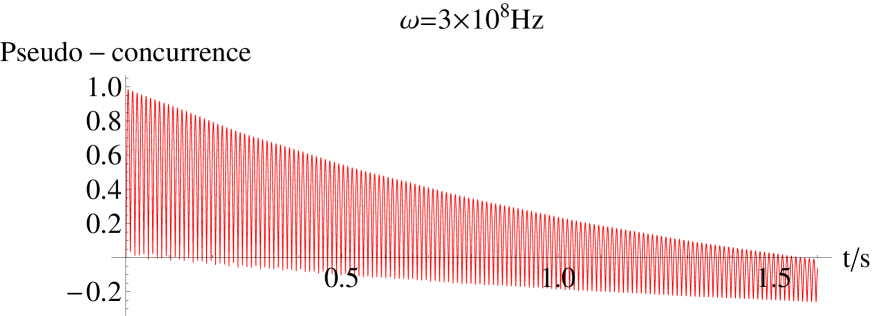
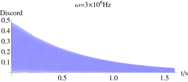
Figure 3: Pseudo-concurrence and quantum discord at frequency $\omega=\frac{\omega_{1}+\omega_{2}}{2}=3\times 10^{8}Hz$.

From Fig.3 we see that, when the evolution time is much shorter than the relaxation scales, the dynamics of entanglement and quantum discord are similar. But for a longer time, namely, near relaxation scales, the entanglement manifests a sequence of sudden deaths and revivals, and finally disappears completely. At the same time, the quantum discord, after a sequence of oscillations, still retains remarkable values.

In a dynamical process, the phenomenon of entanglement disappears in a finite time is named entanglement sudden death [26]. This is an interesting phenomenon in contrast to the usual intuition that decoherence will be in an infinite time. Also, this is an important phenomenon for quantum information processing since much of quantum information processing rely on entanglement [1, 2].

5 Summary

In summary, we investigated the dynamics of entanglement and quantum discord of two qubits in liquid state homonuclear NMR systems. We showed that the dynamical behaviors of entanglement and quantum discord are similar in short time where relaxation effects can be neglected. When the time is long enough to be comparable to the relaxation rates, the entanglement manifests the phenomenon of sudden deaths and survivals, and at last disappears completely. Meanwhile the quantum discord retains remarkable values. That is to say, quantum discord is more robust than entanglement against the relaxation processes. Hence quantum algorithms based only on quantum discord correlation may be more robust than those based on entanglement.

Appendix A Explicit expressions for $\{x_{i}\}_{i=1}^{3}$ and $\{T_{ij}\}_{i,j=1}^{3}$ by the elements of $\rho$ in Eq.(11)

$x_{1}=\rho_{13}+\rho_{24}+\rho_{31}+\rho_{42}$

$x_{2}=i(\rho_{13}+\rho_{24}-\rho_{31}-\rho_{42})$

$x_{3}=\rho_{11}+\rho_{22}-\rho_{33}-\rho_{44}$

$T_{11}=\rho_{14}+\rho_{23}+\rho_{32}+\rho_{41}$

$T_{12}=i(\rho_{14}-\rho_{23}+\rho_{32}-\rho_{41})$

$T_{13}=\rho_{13}-\rho_{24}+\rho_{31}-\rho_{42}$

$T_{21}=i(\rho_{14}+\rho_{23}-\rho_{32}-\rho_{41})$

$T_{22}=-\rho_{14}+\rho_{23}+\rho_{32}-\rho_{41}$

$T_{23}=i(\rho_{13}-\rho_{24}-\rho_{31}+\rho_{42})$

$T_{31}=\rho_{12}+\rho_{21}-\rho_{34}-\rho_{43}$

$T_{32}=i(\rho_{12}-\rho_{21}-\rho_{34}+\rho_{43})$

$T_{33}=\rho_{11}-\rho_{22}-\rho_{33}+\rho_{44}$

Appendix B Explicit expression of matrix A in Eq.(39)

For simplicity, we put $\frac{\omega_{1}+\omega_{2}}{2}=a$, $\frac{\omega_{1}-\omega_{2}}{2}=b$, $J=c$, $\frac{g_{1}}{2}=d$, $\frac{g_{2}}{2}=e$, then

$A=i\{\{0,-e,-d,0,e,0,0,0,d,0,0,0,0,0,0,0\},$

$\ \ \ \ \ \ \ \ \ \{-e,a-y-b-2c,0,-d,0,e,0,0,0,d,0,0,0,0,0,0\},$

$\ \ \ \ \ \ \ \ \ \{-d,0,a-y+b-2c,-e,0,0,e,0,0,0,d,0,0,0,0,0\},$

$\ \ \ \ \ \ \ \ \ \{0,-d,-e,2a-2y,0,0,0,e,0,0,0,d,0,0,0,0\},$

$\ \ \ \ \ \ \ \ \ \{e,0,0,0,-a+y+b+2c,-e,-d,0,0,0,0,0,d,0,0,0\},$

$\ \ \ \ \ \ \ \ \ \{0,e,0,0,-e,0,0,-d,0,0,0,0,0,d,0,0\},$

$\ \ \ \ \ \ \ \ \ \{0,0,e,0,-d,0,2b,-e,0,0,0,0,0,0,d,0\},$

$\ \ \ \ \ \ \ \ \ \{0,0,0,e,0,-d,-e,a-y+b+2c,0,0,0,0,0,0,0,d\},$

$\ \ \ \ \ \ \ \ \ \{d,0,0,0,0,0,0,0,-a+y-b+2c,-e,-d,0,e,0,0,0\},$

$\ \ \ \ \ \ \ \ \ \{0,d,0,0,0,0,0,0,-e,-2b,0,-d,0,e,0,0\},$

$\ \ \ \ \ \ \ \ \ \{0,0,d,0,0,0,0,0,-d,0,0,-e,0,0,e,0\},$

$\ \ \ \ \ \ \ \ \ \{0,0,0,d,0,0,0,0,0,-d,-e,a-b+2c-y,0,0,0,e\},$

$\ \ \ \ \ \ \ \ \ \{0,0,0,0,d,0,0,0,e,0,0,0,-2a+2y,-e,-d,0\},$

$\ \ \ \ \ \ \ \ \ \{0,0,0,0,0,d,0,0,0,e,0,0,-e,-a-b-2c+y,0,-d\},$

$\ \ \ \ \ \ \ \ \ \{0,0,0,0,0,0,d,0,0,0,e,0,-d,0,-a+b-2c+y,-e\},$

$\ \ \ \ \ \ \ \ \ \{0,0,0,0,0,0,0,d,0,0,0,e,0,-d,-e,0\}\}$

$\ \ \ \ \ -DiagonalMatrix[\{\frac{1}{T_{1}},\frac{1}{T_{2}},\frac{1}{T_{2}},\frac{1}{T_{2}},\frac{1}{T_{2}},\frac{1}{T_{1}},\frac{1}{T_{2}},\frac{1}{T_{2}},\frac{1}{T_{2}},\frac{1}{T_{2}},\frac{1}{T_{1}},\frac{1}{T_{2}},\frac{1}{T_{2}},\frac{1}{T_{2}},\frac{1}{T_{2}},\frac{1}{T_{1}}\}].$

References

• [1] M. A. Nielsen and I. L. Chuang, Quantum Computation and Quantum Information, Cambridge University Press, Cambridge, England, 2000.
• [2] R. Horodecki et al., Rev. Mod. Phys. 81 (2009) 865.
• [3] E. Knill and R. Laflamme, Phys. Rev. Lett. 81 (1998) 5672.
• [4] A. Datta, A. Shaji, and C. M. Caves, Phys. Rev. Lett. 100 (2008) 050502.
• [5] B. P. Lanyon, M. Barbieri, M. P. Almeida, and A. G. White, Phys. Rev. Lett. 101 (2008) 200501.
• [6] H. Ollivier and W. H. Zurek, Phys. Rev. Lett. 88 (2001) 017901.
• [7] L. Henderson and V. Vedral, J. Phys. A 34 (2001) 6899.
• [8] R. Dillenschneider, Phys. Rev. B 78 (2008) 224413; M. S. Sarandy, Phys. Rev. A 80 (2009) 022108.
• [9] J. Cui and H. Fan, e-print arXiv:0904.2703.
• [10] T. Werlang, S. Souza, F. F. Fanchini, and C. J. Villas Boas, Phys. Rev. A 80 (2009) 024103.
• [11] T. Werlang and G. Rigolin, Phys. Rev. A 81 (2010) 044101.
• [12] B. Wang, Z.-Y. Xu, Z.-Q. Chen, and M. Feng, Phys. Rev. A 81 (2010) 014101.
• [13] L. M. K. Vandersypen and I. L. Chuang, Rev. Mod. Phys. 76 (2005) 1037.
• [14] I. S. Oliveira, T. J. Bonagamba, R. S. Sarthour, J. C. C. Freitas, and E. R. deAzevedo, NMR Quantum Information Processing, Elsevier, Amsterdam, 2007.
• [15] A. F. Fahmy, R. Marx, W. Bermel, and S. J. Glaser, Phys. Rev. A 78 (2008) 022317.
• [16] G. B. Furman, V. M. Meerovich, and V. L. Sokolovsky, Phys. Rev. A 78 (2008) 042301.
• [17] E. Rufeil-Fiori, C. M. S nchez, F. Y. Oliva, H. M. Pastawski, and P. R. Levstein, Phys. Rev. A 79 (2009) 032324.
• [18] Y. Ota, Y. Goto, Y. Kondo, and M. Nakahara, Phys. Rev. A 80 (2009) 052311.
• [19] W. Zhang, P. Cappellaro, N. Antler, B. Pepper, D. G. Cory, V. V. Dobrovitski, C. Ramanathan, and L. Viola, Phys. Rev. A 80 (2009) 052323.
• [20] D. O. Soares-Pinto, L. C. C leri, R. Auccaise, F. F. Fan-chini, E. R. deAzevedo, J. Maziero, T. J. Bonagamba, and R. M. Serra, Phys. Rev. A 81 (2010) 062118.
• [21] W. K. Wootters, Phys. Rev. Lett. 80 (1998) 2245.
• [22] S. Luo, Phys. Rev. A 77 (2008) 042303.
• [23] M. Ali, A. R. P. Rau and G. Alber, Phys. Rev. A 81 (2010) 042105.
• [24] B. Dakic , V. Vedral and C. Brukner, Phys. Rev. Lett. 105 (2010) 190502.
• [25] H.O. Wijewardane, C.A. Ullrich, Appl. Phys. Lett. 84 (2004) 3984.
• [26] T. Yu and J. H. Eberly, Phys. Rev. Lett. 93 (2004) 140404.