The Fulde-Ferrell-Larkin-Ovchinnikov states for the d-wave superconductor in the two-dimensional orthorhombic lattice

Abstract

The Fulde-Ferrell-Larkin-Ovchinnikov (FFLO) state of a two-dimensional (2D) orthorhombic lattice superconductor is studied based on the Bogoliubov-de-Gennes equations. It is illustrated that the 2D FFLO state is suppressed and only one-dimensional (1D) stripe state is stable. The stripe changes its orientation with the increasing Zeeman field. There exists a crossover region where the gap structure has some local 2D features. These results are significantly different from those of the tetragonal lattice system. The local density of states is also studied which can be checked and compared with experiments in future.

The Fulde-Ferrell-Larkin-Ovchinnikov (FFLO) state, known as the finite momentum of the Copper pair, was predicted in the mid of 1960sFulde1964 ; Larkin1964 . It will occur when the Pauli paramagnetism effect dominates over the orbital effectGruenberg1966 . Thus the low dimensional layered superconducting (SC) materials with the magnetic field parallel to the SC layers are the strong candidates to realize the FFLO state. Recently, signatures for possible FFLO state have been found in various crystal systems, such as the heavy fermion materials $\mathrm{CeCoIn_{5}}$,Radovan2003 ; Bianchi2003 ; Kumagai2006 the organic superconductors $\mathrm{\lambda-(BETS)_{2}GaCl_{4}}$,Tanatar2002 $\mathrm{\lambda-(BETS)_{2}FeCl_{4}}$Uji2001 ; Balicas2001 , $\mathrm{\kappa-(BEDT-TTF)_{2}Cu(NCS)_{2}}$,Shimahara1997 ; Manalo2000 and the iron-based materials LiFeAs.Cho On the other hand, the realization of FFLO state in the cold atom system is studied intensivelyLoh2010 ; Koponen2007 ; Cai2010 ; Koponen2008 ; Parish2007 and recently the experimental signatures are found in the one-dimensional optical lattice.Liao2010

The experimental development for the FFLO state in low dimensional systems has attracted much attention. Theoretically the calculation based on the lattice model is of great interest and the results may compare with the experimental results of the crystal systems or the cold atom system. One of the fundamental issues of the FFLO state is the detailed gap structure, which can be studied through minimizing the free energyCombescot2005 , or through the self-consistent calculation based on the Eilenberger equation.Vorontsov2005 ; Mora2004 At the mean time, the Bogoliubov-de-Gennes (BdG) technique has been a powerful tool to study various imhomogenous SC states and it can also obtain the SC order parameter self-consistently. Thus it is also an effective tool to study the FFLO state especially in lattice system. Previously, based on the BdG equations, the FFLO state was studied intensively in the tetragonal lattice system. Many groups have reported their results and numerically the gap structure depends on the pairing symmetry.Wang2006 ; Wang2007 ; Cui2008 ; Zuo2009 ; Zhou2009 For $s$-wave pairing symmetry, the one-dimensional (1D) stripe-like pattern was reported.Wang2006 ; Cui2008 For $d$-wave paring symmetry, recently it was proposed that a transition from the 1D stripe-like pattern to the two-dimensional (2D) checkerboard pattern will occur as the exchange field increases.Zhou2009 And the 2D pattern may change to the 1D pattern in presence of the impurities.Wang2007 ; Zuo2009

The above results of the gap structure for the tetragonal lattice system are significantly different from the previous theoretical results in the isotropic systems,Shimahara1998 ; Maki2002 as discussed by Ref.[26], indicating that the intrinsic symmetry of the crystal lattice should play an important role in the gap structure of the FFLO states. For a real SC material, there often exists a structural transition from tetragonal- to orthorhombic-lattice with the variation of the doping level. Some possible microscopic orders, such as the stripe orderKivelson2003 or the nematic orderHinkov2008 ; Daou2010 ; Doh2007 ; Vojta2010 may also lead to a weak anisotropy in the ab-plane. Furthermore, the 1D FFLO stripe in the tetragonal lattice itself may induce the in-plane anisotropy. Therefore, the studies of the FFLO states in an orthorhombic lattice system is of great interest while so far little attention is paid to the FFLO state on this system.

In this paper, motivated by the above consideration, we calculate the spatially distributed order parameter self-consistently based on the BdG equations on a 2D lattice with $x-y$ anisotropic hopping. Our results show that the 2D solution of the SC gap structure will be suppressed and disappears as the orthorhombicity strength $\gamma\equiv{t_{x}}/t_{y}$ increases. For the case of $\gamma=1.05$, only stable 1D stripe state exists and it is also found that the stripe changes its orientation with the increasing Zeeman field. A crossover region exists between these two stripe states and some local 2D features are obtained in this region. The local density of states (LDOS) is also studied to distinguish the different states.

We start from the model on the 2D lattice with the Zeeman splitting effect. The model Hamiltonian can be written as,

$$H= -\sum_{ij\sigma}(t_{ij}c_{i\sigma}^{\dagger}c_{j\sigma}+\mathrm{H.c.})-\sum_{i\sigma}(\mu+\sigma{h})c_{i\sigma}^{\dagger}c_{i\sigma}$$ (1)

$$+\sum_{ij}(\Delta_{ij}c_{i\uparrow}^{\dagger}c_{j\downarrow}^{\dagger}+\mathrm{H.c.}),$$

where $t_{ij}$ are the hopping constants and $\mu$ is the chemical potential. $\sigma{h}$ is the Zeeman energy term, caused by the in-plane magnetic field, with $\sigma=\pm 1$ representing the spin-up and spin-down electrons respectively.

This Hamiltonian can be diagonalized by solving the BdG equations,

$$\sum_{j}\left(\begin{array}[]{cc}H_{ij}&\Delta_{ij}\\ \Delta^{*}_{ij}&-H^{*}_{ij}\end{array}\right)\left(\begin{array}[]{c}u^{n}_{j\uparrow}\\ v^{n}_{j\downarrow}\end{array}\right)=E_{n}\left(\begin{array}[]{c}u^{n}_{i\uparrow}\\ v^{n}_{i{\downarrow}}\end{array}\right),$$ (2)

where $H_{ij}$ is expressed by

$$H_{ij}=-t_{ij}-(\mu+\sigma{h})\delta_{ij}.$$ (3)

The SC order parameter and the local electron density $n_{i}$ are obtained self-consistently:

$$\Delta_{ij}=\frac{V_{ij}}{4}\sum_{n}(u_{i\uparrow}^{n}\upsilon_{j\downarrow}^{n*}+u_{j\uparrow}^{n}\upsilon_{i\downarrow}^{n*})\mathrm{tanh}\bigg{(}\frac{E_{n}}{2k_{B}T}\bigg{)},$$ (4)

$$n_{i}=\sum_{n}|u_{i\uparrow}^{n}|^{2}f(E_{n})+\sum_{n}|\upsilon_{i\downarrow}^{n}|^{2}[1-f(E_{n})].$$ (5)

Here $f(x)$ is the Fermi distribution function. $V_{ij}$ is the pairing strength. In the present work, we consider the nearest neighbor (NN) pairing with $V_{ij}=V\delta_{i,j\pm\hat{\alpha}}$. For the tetragonal lattice system the NN pairing will reproduce the $d_{x^{2}-y^{2}}$-pairing symmetry. The $d$-wave order parameter at the site $i$ can be defined as $\Delta^{d}_{i}=1/4(\Delta_{i,i+\hat{x}}+\Delta_{i,i-\hat{x}}-\Delta_{i,i+\hat{y}}-\Delta_{i,i-\hat{y}})$. For the case of orthorhombic lattice the four-fold symmetry is broken so that a $s$-wave component will be induced and is expected to increase as the orthorhombicity strength $\gamma$ increases. The $s$-wave component is defined as $\Delta^{s}_{i}=1/4(\Delta_{i,i+\hat{x}}+\Delta_{i,i-\hat{x}}+\Delta_{i,i+\hat{y}}+\Delta_{i,i-\hat{y}})$. Since we consider only weak $x-y$ isotropy in the present work with $\gamma\leq 1.05$. Our numerical results show that the $s$-wave component is quite small [$\Delta^{s}/\Delta^{d}<0.03$]. Thus in our following presented results we neglect the small $s$-wave component and use the above $d$-wave order parameter as the definition of the on-site order parameter. We also define the The magnetization $m_{i}$ as $m_{i}=\langle{S^{z}_{i}}\rangle=\hbar/2\langle{n_{i\uparrow}}-n_{i\downarrow}\rangle$.

The LDOS is expressed by

$$\rho_{i}(\omega)=\sum_{n}[|u_{i\uparrow}^{n}|^{2}\delta(E_{n}-\omega)+|\upsilon_{i\downarrow}^{n}|^{2}\delta(E_{n}+\omega)],$$ (6)

where the delta function $\delta(x)$ has been approximated by $\Gamma/\pi(x^{2}+\Gamma^{2})$ with $\Gamma=0.02$.

In the following calculation, we consider the NN hopping with the hopping constant in $x$ direction being $t_{x}=1.0$ and that in $y$ direction $t_{y}=t_{x}/\gamma$. Here, $\gamma$ represents the orthorhombicity strength. The pairing potential $V$ and the filling electron density $n$ are chosen as $V=1.3$ and $n=0.84$ (hole-doped samples with doping $\delta=0.16$). The calculation is made on a $48\times 48$ lattice with the periodic boundary condition, and the randomly distributed initial values of the order parameters are chosen. The $10\times 10$ supercell is used to calculate the LDOS.

Figure 1: Phase diagram of an 2D orthorhombic lattice superconductor in the parallel magnetic field. $h=g\mu_{B}H$ is the exchange field and $\gamma$ the orthorhombicity strength. The crossover region is indicated by the shadow.

Our main results are summarized in Fig. 1, where the phase diagram is plotted. As one can see, for low anisotropy, the whole SC state is divided into three regions, namely, the uniform SC state, the 1D FFLO state, and the 2D FFLO state, which is consistent with the previous results.Zhou2009 For $\gamma=1.05$ and at low fields, the SC state still includes the uniform SC state and the 1D FFLO state. At $0.22\leq{h}<0.23$, as indicated by the shadow, there exists a crossover region. In this region, the gap structure forms the coexistence of the 1D stripe-like pattern and some local 2D features. As the exchange field increases further, as seen, another 1D FFLO state shows up. The orientation of the stripe pattern is different from that of the low field, namely, for the lower field FFLO state the stripe is parallel to the $x$ direction (stripe I) and that of the higher field one is parallel to the $y$ direction (stripe II). We also note that the upper critical field $H_{c2}$ increases with the increasing $\gamma$.

We now studied the self-consistent results of the order parameter and magnetization with $\gamma=1.05$ in Fig.2. The order parameters are plotted in Figs.2(a)-2(e). As seen, for the weaker magnetic field, the order parameter is uniform [Fig. 2(a)]. The SC order forms the stripe pattern as the exchange field increases to 0.2, as seen in Fig.2(b). The periodicity of the order parameter is about 24 along $y$ direction as $h=0.20$, which is consistent with the previous results.Zhou2009 For the case of $h=0.22$ and $h=0.225$, a crossover region from stripe I state to stripe II state occurs, indicated in Figs. 2(c) and 2(d). As seen in Fig. 2(c), the gap structure has some 2D features around the point ’A’ with the stripe II state showing up gradually. For $h=0.225$ [Fig. 2(d)], the stripe II state dominates over the stripe I one and the 2D FFLO features are almost suppressed. As $h$ increases further, i.e. for $h=0.23$, the SC order forms the stripe pattern again with the stripe parallelling to the $y$ axis.

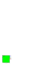
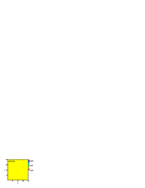
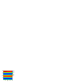
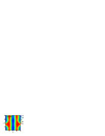
Figure 2: (Color online) Plots of the order parameter $\Delta$ and and the magnetization $m_{i}$ as a function of position for various Zeeman fields $h$ with $T=10^{-5}$ at anisotropic hopping parameter $\gamma=1.05$.

The spatial distributions of the magnetization (with the units $\hbar$) are shown in Figs. 2(f)-2(j). As seen in Fig. 2(f), in the uniform phase, the distribution is also uniform, where the magnetization is very weak (about 0.0017) due to the suppression by the SC order. In the 1D FFLO stripe I state, as seen in Fig. 2(g), the pattern also forms 1D stripe but the periodicity is only half of that of the order parameter. The intensity is largest along the nodal lines and is suppressed when the SC order parameter increases. It reaches the minimum value as the SC order is maximum. These features are similar to previous results in tetragonal lattice system Zhou2009 . In the crossover region, such as $h=0.22$, the magnetization also behaves the coexistence of the 1D and 2D character. As $h$ increasing further, the magnetization forms 1D stripe again with the orientation changing from $y$ axis to $x$ axis.

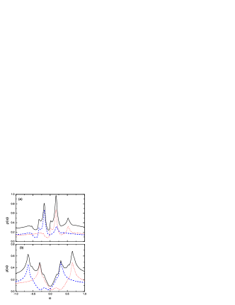
Figure 3: (Color online) The LDOS spectra for 1D stripe I state at $h=0.17$. Panel (a) and (b) are the LDOS spectra at the nodal line and at the site where the order parameter is maximum, respectively. The (blue) dashed and (red) dotted lines, and the (black) solid line are spin-up LDOS, spin-down LDOS, and whole LDOS, respectively.

Now let us study the LDOS spectra. The LDOS from Eq.6 includes two terms, i.e., the spin-up LDOS and spin-down LDOS, respectively. In presence of the Zeeman field, due to the Pauli paramagnetic effect, the spin-up LDOS and spin-down one sperate with the spin-up one shifting to the left and the spin-down one to the right, respectively. The calculated LDOS spectra in the uniform phase are similar to the previous report,Zhou2009 which is not shown here. The LDOS spectra in the 1D stripe I phase with $h=0.17$ are shown in Fig. 3. Fig. 3(a) is for the site on the nodal line. As seen, the spin-up LDOS spectra show two low-energy peaks locating at $\omega=-0.17$ and $-0.32$. The SC coherent peak is suppressed. The spin-down LDOS shifts to the right with the two low-energy peaks at $\omega=0.02$ and $0.17$. These in-gap peaks originate from the finite energy Andreev bound states due to the sign change in the order parameter across the nodal lines, which is the signature of 1D FFLO state, as also discussed previously Wang2006 ; Zhou2009 . The peaks at the negative energy in total LDOS comes from the spin-up LDOS and the peaks at the positive energy are contributed by the spin-down LDOS. The intensity of the in-gap peaks will decrease as the site moves away from the nodal line. As seen from Fig. 3(b), at the site where the order parameter is maximum, the in-gap peaks are turned to be a hump at the midgap position for both spin-up and spin-down LDOS spectra. The SC coherent peaks are seen clearly. The midgap hump is so weak that it is concealed in the whole LDOS spectrum.

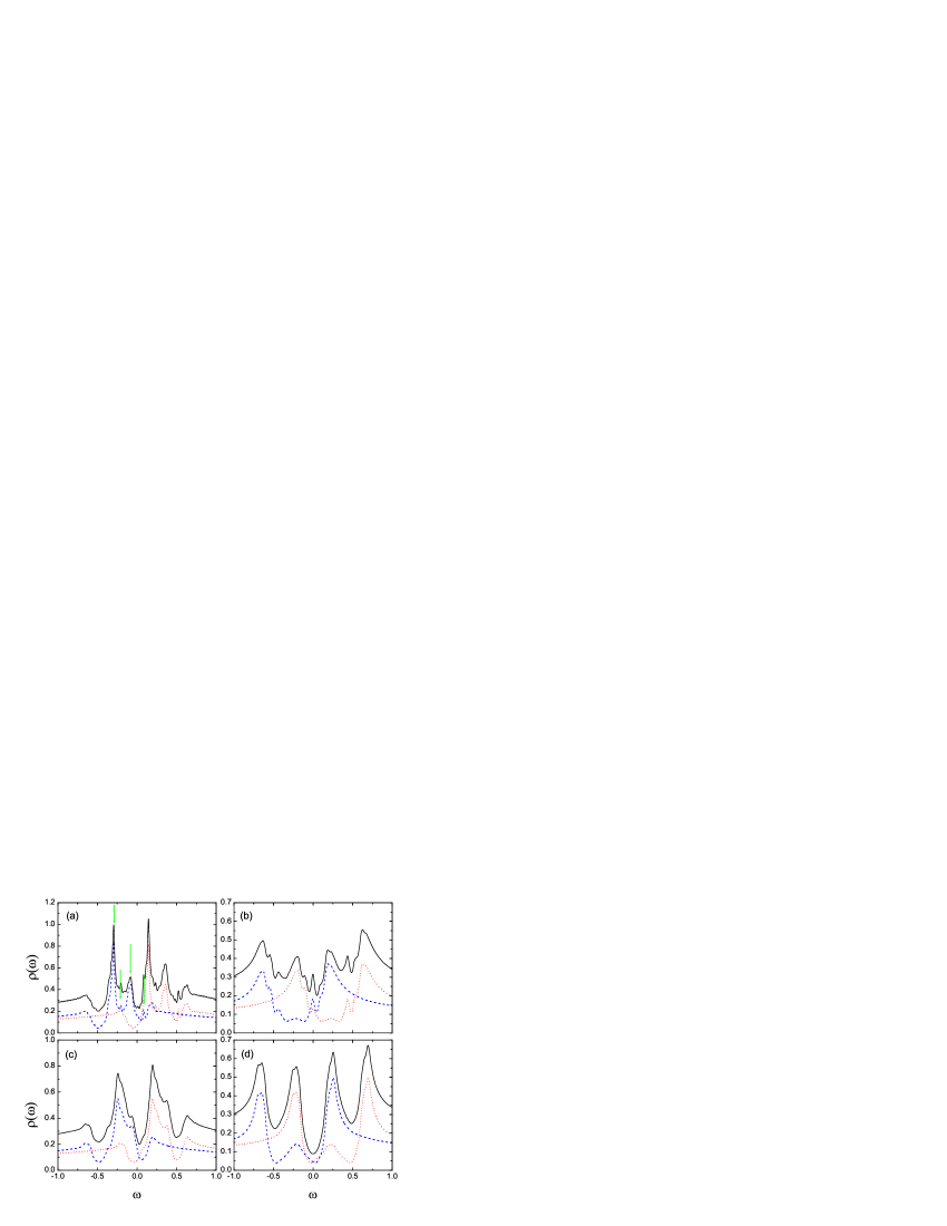
Figure 4: (Color online) The LDOS spectra in the crossover region with $h=0.22$. Panel (a) is the spectrum at the saddle ponit where two nodal lines intersect. Panel (b) is the spectrum at the site where the order parameter is maximum in the 2D FFLO region. Panels (c) and (d) are the spectra at the nodal line and at the site where the order parameter is maximum in the 1D FFLO region, respectively. The (blue) dashed and (red) dotted lines, and the (black) solid line are spin-up LDOS, spin-down LDOS, and whole LDOS, respectively.

The LDOS spectra for the crossover region with $h=0.22$ are presented in Fig.4. The spectrum at the saddle point in the local 2D FFLO region [near the point ”A” in Fig. 2(c)] is presented in Fig. 4(a). Although the gap structure is quite different from previous results in tetragonal lattice system. While actually for this case the spectrum is similar to that of the saddle point’s spectrum in the 2D checkerboard FFLO state Wang2006 ; Zhou2009 , namely, two kinds of Andreev bound states exist. As a result, four in-gap peaks exist in the spin-up LDOS spectra at the energies -0.300, -0.208, -0.052, and 0.081 (indicated by the arrows). At the site where the order parameter is maximum, the LDOS spectrum [Fig. 4(b)] is very complicated, while the two coherence peaks outside can be seen clearly. Shown in Fig. 4(c) is the LDOS spectrum on the nodal line in the 1D FFLO region. There are also two in-gap peaks in both the spin-up and spin-down LDOS spectra, indicating the 1D characteristics. The SC coherent peaks are suppressed again, similar to the case of 1D stripe phase [Fig. 3(a)]. At the site where the order parameter is maximum [Fig. 4(d)], the in-gap peaks are turned to be a hump at the midgap position for both the spin-up and spin-down LDOS spectra, while the SC coherence peaks are clearly seen, which leads to the four peaks in the whole LDOS spectrum. Summing up the above results, it is found that in the crossover region, the FFLO indeed includes both the 1D and 2D FFLO characters, which is consistent with the spatial distribution of the order parameter and the magnetization (Fig. 2).

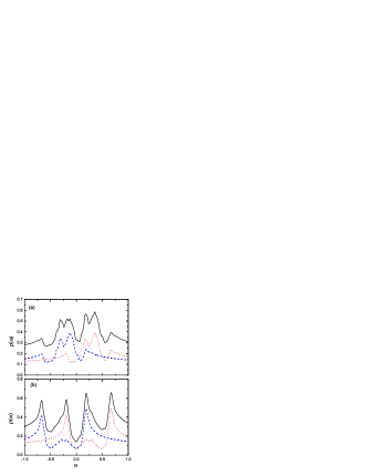
Figure 5: (Color online) Similar to Fig. 3, but for h=0.24.

The LDOS spectra of the 1D stripe II state with $h=0.24$ is presented in Fig. 5. The result at the nodal line is shown in Fig. 5(a). It can be seen that there are two in-gap peaks of both the spin-up and spin-down LDOS, while the SC coherence peaks are suppressed. Presented in Fig. 5(b) is the LDOS spectrum at the site where the order parameter is maximum. It is found that the in-gap peaks are almost suppressed completely, while the SC coherence peaks are clearly seen. Thus, the feature of the LDOS spectra of the 1D stripe II state is similar to that of the 1D stripe I state.

We have shown the LDOS spectra of the three different phases, namely the 1D strip 1 phase, the crossover region, and the 1D stripe II phase. As seen in Fig. 4(a)-4(d), the spectra of the Q2D state are quite different from that of the other two 1D stripe phases. In the Q2D state, the 1D and 2D FFLO states coexist in different regions. These features are expected to be detected by the scanning tunneling microscopy (STM) experiments.

Figure 6: (Color online) The LDOS maps for quasiparticles with $\omega=0$ and different exchange fields.

To distinguish the two stripe phases, we present the LDOS images with $\omega=0$. Shown in Fig. 6(a) is the LDOS image at $h=0.20$ in the 1D stripe I state. As seen, in this state it also forms 1D stripe-like pattern similar to the spatial distribution of the order parameter but the periodicity is only half of that of the order parameter. The intensity is largest along the nodal lines and is suppressed when the SC order parameter increases. It reaches the minimum value as the SC order is maximum. The stripe parallels to the $x$ axis, consistent with the gap structure. The images in the crossover region are presented in Figs. 6(b) and 6(c) with $h=0.22$ and $h=0.225$, respectively. As seen from Fig. 6(b), the LDOS image in this state also behaves the Q2D characteristics, i.e., the stripe-like and the local 2D patterns coexist. The intensity is largest at the saddle points where two nodal lines intersect. It reaches the minimum value as the SC order is maximum. The LDOS image at $h=0.23$ in the 1D stripe II phase is presented in Fig. 6(d). It is found that the image forms stripe-like pattern again with the orientation switching to the $y$ axis. Therefore, it can be used to distinguish the two stripe phases by the STM experiments.

In summary, based on the BdG equations and the $d$-wave superconductivity, the phase diagram and the order-parameter structure is studied in presence of the external exchange field of a 2D orthorhombic lattice superconductor. It is found that for weak anisotropic hoping, i.e. $\gamma=1.05$, the 2D FFLO state is suppressed and only the 1D state exists. The orientation of the stripe changes as the exchange field increases. The local Q2D state exists in the crossover region. These results are much different from those of the tetragonal lattice system. Our result suggests that the symmetry of the lattice plays an important role in the gap structure of the FFLO state. The local Q2D state can be detected by the STM experiments according to the calculated spectra of LDOS. The LDOS images with $\omega=0$ in these phases are also presented, which can be used to distinguish the different phases.

We thank Dr. Chen Wei and Dr. Xue Hongtao for the technical support. This work was supported by the Scientific Research Foundation from Nanjing University of Aeronautics and Astronautics.

References

- (1) P. Fulde and R. A. Ferrell, Phys. Rev. 135, A550 (1964).
- (2) A. I. Larkin and Yu. N. Ovchinnikov, Zh. Eksp. Teor. Fiz. 47, 1136 (1964) [Sov. Phys. JETP 20, 762 (1965)].
- (3) L. W. Gruenberg and L. Gunther, Phys. Rev. Lett. 16, 996 (1966).
- (4) H. A. Radovan, N. A. Fortune, T. P. Murphy, S. T. Hannahs, E. C. Palm, S. W. Tozer, and D. Hall, Nature (London) 425, 51 (2003).
- (5) A. Bianchi, R. Movshovich, C. Capan, P. G. Pagliuso, and J. L. Sarrao, Phys. Rev. Lett. 91, 187004 (2003).
- (6) K. Kumagai, M. Saitoh, T. Oyaizu, Y. Furukawa, S. Takashima, M. Nohara, H. Takagi, and Y. Matsuda, Phys. Rev. Lett. 97, 227002 (2006).
- (7) M. A. Tanatar, T. Ishiguro, H. Tanaka, and H. Kobayashi, Phys. Rev. B 66, 134503 (2002).
- (8) S. Uji, H. Shinagawa, T. Terashima, T. Yakabe, Y. Terai, M. Tokumoto, A. Kobayashi, H. Tanaka, and H. Kobayashi, Nature (London) 410, 908 (2001).
- (9) L. Balicas, J. S. Brooks, K. Storr, S. Uji, M. Tokumoto, H. Tanaka, H. Kobayashi, A. Kobayashi, V. Barzykin, and L. P. Gorkov, Phys. Rev. Lett. 87, 067002 (2001).
- (10) H. Shimahara, J. Phys. Soc. Jpn. 66, 541 (1997).
- (11) S. Manalo and U. Klein, J. Phys.: Condens. Matter 12, L471 (2000).
- (12) K. Cho, H. Kim, M. A. Tanatar, Y. J. Song, Y. S. Kwon, W. A. Coniglio, C. C. Agosta, A. Gurevich, and R. Prozorov, Phys. Rev. B 83, R060502 (2011).
- (13) Zi Cai, Yupeng Wang, and Congjun Wu, arXiv:1009.3257.
- (14) Y. L. Loh and N. Trivedi, Phys. Rev. Lett. 104, 165302 (2010).
- (15) T. K. Koponen, T. Paananen, J. P. Martikainen, and P. Törmä, Phys. Rev. Lett. 99, 120403 (2007).
- (16) T. K. Koponen, T. Paananen, J. P. Martikainen, M. R. Bakhtiari and P. Törmä,, N. J. Phys. 10, 045014 (2008).
- (17) M. M. Parish, S. K. Baur, E. J. Mueller, and D. A. Huse, Phys. Rev. Lett. 99, 250403 (2007).
- (18) Yean-an Liao, Ann Sophie C. Rittner, Tobias Paprotta, Wenhui Li, Guthrie B. Partridge, Randall G. Hulet, Stefan K. Baur and Erich J. Mueller, Nature (London) 467 567 (2010).
- (19) R. Combescot and C. Mora, Phys. Rev. B 71, 144517 (2005).
- (20) A. B. Vorontsov, J. A. Sauls, and M. J. Graf, Phys. Rev. B 72, 184501 2005.
- (21) C. Mora and R. Combescot, Europhys. Lett. 66, 833 (2004).
- (22) Qian Wang, H.-Y. Chen, C.-R. Hu, and C. S. Ting, Phys. Rev. Lett. 96, 117006 (2006).
- (23) Q. Cui and K. Yang, Phys. Rev. B 78, 054501 (2008).
- (24) Q. Wang, C.-R. Hu, and C.-S. Ting, Phys. Rev. B 75, 184515 (2007).
- (25) X.-J. Zuo and C.-D. Gong, EPL 86, 47004 (2009).
- (26) Tao Zhou and C. S. Ting, Phys. Rev. B 80, 224515 (2009).
- (27) H. Shimahara, J. Phys. Soc. Jpn. 67, 736 (1998).
- (28) K. Maki and H. Won, Physica B (Amsterdam) 322, 315 (2002).
- (29) S. A. Kivelson, I. P. Bindloss, E. Fradkin, V. Oganesyan, J. M. Tranquada, A. Kapitulnik, and C. Howald, Rev. Mod. Phys. 75, 1201 (2003).
- (30) V. Hinkov, D. Haug, B. Fauqu e, P. Bourges, Y. Sidis, A. Ivanov, C. Bernhard, C. T. Lin, and B. Keimer, Science 319, 597 (2008).
- (31) R. Daou, J. Chang, D. LeBoeuf, O. Cyr-Choiniere, F. Laliberte, N. Doiron-Leyraud, B. J. Ramshaw, R. Liang, D. A. Bonn, W. N. Hardy, and L. Taillefer, Nature 463, 519 (2010).
- (32) Matthias Vojta, Eur. Phys. J. Special Topics 188, 49 (2010).
- (33) Hyeonjin Doh and Hae-Young Kee, Phys. Rev. B 75, 233102 (2007).