KP solitons and total positivity for the Grassmannian

Abstract.

Soliton solutions of the KP equation have been studied since 1970, when Kadomtsev and Petviashvili proposed a two-dimensional nonlinear dispersive wave equation now known as the KP equation. It is well-known that one can use the Wronskian method to construct a soliton solution to the KP equation from each point of the real Grassmannian $Gr_{k,n}$. More recently, several authors [3, 15, 2, 4, 6] have studied the regular solutions that one obtains in this way: these come from points of the totally non-negative part of the Grassmannian $(Gr_{k,n})_{\geq 0}$.

In this paper we exhibit a surprising connection between the theory of total positivity for the Grassmannian, and the structure of regular soliton solutions to the KP equation. By exploiting this connection, we obtain new insights into the structure of KP solitons, as well as new interpretations of the combinatorial objects indexing cells of $(Gr_{k,n})_{\geq 0}$ [25]. In particular, we completely classify the spatial patterns of the soliton solutions coming from $(Gr_{k,n})_{\geq 0}$ when the absolute value of the time parameter is sufficiently large. We demonstrate an intriguing connection between soliton graphs for $(Gr_{k,n})_{>0}$ and the cluster algebras of Fomin and Zelevinsky [9], and we use this connection to solve the inverse problem for generic KP solitons coming from $(Gr_{k,n})_{>0}$. Finally we construct all the soliton graphs for $(Gr_{2,n})_{>0}$ using the triangulations of an $n$-gon.

1. Introduction

The KP equation is a two-dimensional nonlinear dispersive wave equation given by

(1.1) $$\frac{\partial}{\partial x}\left(-4\frac{\partial u}{\partial t}+6u\frac{\partial u}{\partial x}+\frac{\partial^{3}u}{\partial x^{3}}\right)+3\frac{\partial^{2}u}{\partial y^{2}}=0,$$

where $u=u(x,y,t)$ represents the wave amplitude at the point $(x,y)$ in the $xy$-plane for fixed time $t$. The equation was proposed by Kadomtsev and Peviashvili in 1970 to study the transversal stability of the soliton solutions of the Korteweg-de Vries (KdV) equation [13]. The KP equation can also be used to describe shallow water waves, and in particular, the equation provides an excellent model for the resonant interaction of those waves (see [16] for recent progress). The equation has a rich mathematical structure, and is now considered to be the prototype of an integrable nonlinear dispersive wave equation with two spatial dimensions (see for example [23, 1, 7, 22, 12]).

One of the main breakthroughs in the KP theory was given by Sato [27], who realized that solutions of the KP equation could be written in terms of points on an infinite-dimensional Grassmannian. The present paper deals with a real, finite-dimensional version of the Sato theory; in particular, we are interested in solutions that are regular in the entire $xy$-plane, where they are localized along certain rays. We call such solution line-soliton solution, and they can be constructed from a point $A$ of the real Grassmannian [27, 28, 10, 12]. In this paper, we denote by $u_{A}(x,y,t)$ the solution associated to $A$.

Recently several authors have worked on classifying the regular line-soliton solutions [3, 15, 2, 4, 6]. These solutions come from points of the totally non-negative part of the Grassmannian, that is, those points of the real Grassmannian whose Plücker coordinates are all non-negative. They found a large variety of soliton solutions which were previously overlooked by those using the Hirota method of a perturbation expansion [12]. In the generic situation, the asymptotic pattern at $y\to\pm\infty$ of the solution consists of $n$ line-solitons. However, because of the nonlinearity in the KP equation, the interaction pattern of the soliton solutions are very complex. Figure 1 illustrates the time evolution of the pattern of a line-soliton solution. Each figure shows the contour plot of the solution at a fixed time $t$ in the $xy$-plane with $x$ in the horizontal and $y$ in the vertical directions.

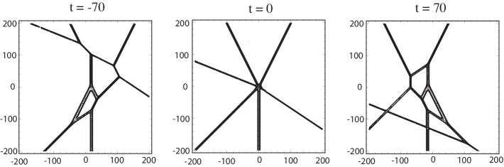
Figure 1. Time evolution of the spatial pattern of a soliton solution. The figures illustrate the contour plots of the solution (see Example 8.16 to reconstruct the figures).

One of the main goals of this paper is to give a combinatorial classification of the patterns generated by the line-soliton solutions as in the figures.

Recently Postnikov [25] studied the totally non-negative part of the Grassmannian $(Gr_{k,n})_{\geq 0}$ from a combinatorial point of view. Total positivity has attracted a lot of interest in the last two decades, largely due to work of Lusztig [19, 20], who introduced the totally positive and non-negative parts of real reductive groups and flag varieties (of which the Grassmannian is an important example). Postnikov gave a decomposition of $(Gr_{k,n})_{\geq 0}$ into positroid cells, by specifying which Plücker coordinates are strictly positive and which are zero. He also introduced several remarkable families of combinatorial objects, including decorated permutations, $\Gamma$ -diagrams, plabic graphs, and Grassmann necklaces, in order to index the cells and describe their properties.

We are interested in the wave pattern generated by a soliton solution $u_{A}(x,y,t)$ in the $xy$-plane for fixed time $t$. We then consider a contour plot $\operatorname{\mathcal{C}}(u_{A},t)$ for each $t$ in the $xy$-plane which is a tropical curve approximating the positions in the plane where the corresponding wave has a peak, see Figure 1.

While the local interactions of arbitrary contour plots are extremely complicated, it is possible to understand their asymptotic structure for $|y|\gg 0$. Moreover, if we take the limit as the time variable $t$ goes to infinity (or more generally, some of the symmetry parameters of the KP equation, denoted by ${\bf t}=(t_{3},t_{4},t_{5},\dots)$ with $t_{3}=t$, also go to infinity), and rescale $x$ and $y$ accordingly, we obtain an asymptotic contour plot, whose combinatorial structure is much more tractable. We then associate to each asymptotic contour plot a soliton graph by forgetting the metric structure of the pattern but remembering the topological structure.

In this paper we establish a tight connection between total positivity on the Grassmannian and the regular soliton solutions of the KP equation. This allows us to apply machinery from total positivity to understand soliton solutions of the KP equation. In particular:

• we classify the soliton graphs and asymptotic contour plots coming from $(Gr_{k,n})_{\geq 0}$ when $t\to\pm\infty$ (Theorems 8.5 and 8.9);

• we demonstrate an intriguing connection between soliton graphs for $(Gr_{k,n})_{>0}$ and the cluster algebras of Fomin and Zelevinsky [9] (Theorem 10.12);

• we solve the inverse problem for KP solitons coming from $(Gr_{k,n})_{>0}$, and from $(Gr_{k,n})_{\geq 0}$ when $|t|\gg 0$ (Theorems 11.4 and 11.2).

• we classify all soliton graphs and asymptotic contour plots coming from $(Gr_{2,n})_{>0}$, and show that these soliton graphs are in bijection with triangulations of a polygon (Theorem 12.2).

Note that prior to our work almost nothing was known about the classification of soliton graphs, except in the cases of $(Gr_{1,n})_{>0}$ [8], and $(Gr_{2,4})_{\geq 0}$ [6].

In the other direction, we give a KP soliton interpretation to nearly all of Postnikov’s combinatorial objects, as well as a new characterization of reduced plabic graphs (Theorem 10.5).

The structure of the paper is as follows. In Sections 2 and 3 we provide background on total positivity on the Grassmannian, and soliton solutions to the KP equation. In Section 4 we explain how to associate soliton graphs to soliton solutions of the KP equation. In the next four sections (Sections 5, 6, 7, and 8) we explain the relationships between combinatorial objects labeling positroid cells and the corresponding soliton solutions. In particular, we explain how (decorated) permutations and Grassmann necklaces control the asympototics of soliton graphs when $|y|\gg 0$, and how $\Gamma$ -diagrams control the soliton graphs at $|t|\gg 0$. We also explain the connection between plabic graphs and soliton graphs. In Section 9 we explain how the existence of $X$-crossings in contour plots corresponds to “two-term” Plücker relations. In Section 10 we prove that generically, the dominant exponentials labeling the regions of a soliton graph for $(Gr_{k,n})_{>0}$ comprise a cluster for the cluster algebra of $Gr_{k,n}$. In Section 11 we address the inverse problem for regular soliton solutions to the KP equation. Finally, in Section 12, we completely classify the soliton graphs coming from solutions $u_{A}$ for $A\in(Gr_{2,n})_{>0}$, and construct them all using triangulations of an $n$-gon.

The present paper provides proofs of the results announced in [17]. In the sequel to this work [18] we have extended many of the results of the present paper from the non-negative part of the Grassmannian to the real Grassmannian. In a future paper we plan to make a detailed study of the relationship between cluster transformations and the evolution of soliton graphs.

Acknowledgements: The authors are grateful for the hospitality of the math departments at UC Berkeley and Ohio State, where some of this work was carried out. They are also grateful to Sara Billey, and to an anonymous referee, whose comments helped them to greatly improve the exposition.

2. Total positivity for the Grassmannian

In this section we review the Grassmannian $Gr_{k,n}$ and Postnikov’s decomposition of its non-negative part $(Gr_{k,n})_{\geq 0}$ into positroid cells [25]. Note that our conventions slightly differ from those of [25].

The real Grassmannian $Gr_{k,n}$ is the space of all $k$-dimensional subspaces of $\mathbb{R}^{n}$. An element of $Gr_{k,n}$ can be viewed as a full-rank $k\times n$ matrix modulo left multiplication by nonsingular $k\times k$ matrices. In other words, two $k\times n$ matrices represent the same point in $Gr_{k,n}$ if and only if they can be obtained from each other by row operations. Let $\binom{[n]}{k}$ be the set of all $k$-element subsets of $[n]:=\{1,\dots,n\}$. For $I\in\binom{[n]}{k}$, let $\Delta_{I}(A)$ denote the maximal minor of a $k\times n$ matrix $A$ located in the column set $I$. The map $A\mapsto(\Delta_{I}(A))$, where $I$ ranges over $\binom{[n]}{k}$, induces the Plücker embedding $Gr_{k,n}\hookrightarrow\mathbb{RP}^{\binom{n}{k}-1}$.

For $\operatorname{\mathcal{M}}\subseteq\binom{[n]}{k}$, the matroid stratum $S_{\mathcal{M}}$ is the set of elements of $Gr_{k,n}$ represented by all $k\times n$ matrices $A$ with $\Delta_{I}(A)\neq 0$ for $I\in\mathcal{M}$ and $\Delta_{J}(A)=0$ for $J\notin\mathcal{M}$. The decomposition of $Gr_{k,n}$ into the strata $S_{\mathcal{M}}$ is called the the matroid stratification.

Definition 2.1.

The totally non-negative Grassmannian $(Gr_{k,n})_{\geq 0}$ (respectively, totally positive Grassmannian $(Gr_{k,n})_{>0}$) is the subset of $Gr_{k,n}$ that can be represented by $k\times n$ matrices $A$ with all $\Delta_{I}(A)$ non-negative (respectively, positive).

Postnikov [25] studied the decomposition of $(Gr_{k,n})_{\geq 0}$ induced by the matroid stratification. More specifically, for $\operatorname{\mathcal{M}}\subseteq\binom{[n]}{k}$, he defined the positroid cell $S_{\mathcal{M}}^{tnn}$ as the set of elements of $(Gr_{k,n})_{\geq 0}$ represented by all $k\times n$ matrices $A$ with $\Delta_{I}(A)>0$ for $I\in\mathcal{M}$ and $\Delta_{J}(A)=0$ for $J\not\in\mathcal{M}$. It turns out that each nonempty $S_{\mathcal{M}}^{tnn}$ is actually a cell [25], and that this decomposition of $(Gr_{k,n})_{\geq 0}$ is a CW complex [26]. Note that $(Gr_{k,n})_{>0}$ is a positroid cell; it is the unique positroid cell in $(Gr_{k,n})_{\geq 0}$ of top dimension $k(n-k)$. Postnikov showed that the cells of $(Gr_{k,n})_{\geq 0}$ are naturally labeled by (and in bijection with) the following combinatorial objects [25]:

• Grassmann necklaces $\mathcal{I}$ of type $(k,n)$

• decorated permutations $\pi^{:}$ on $n$ letters with $k$ weak excedances

• equivalence classes of reduced plabic graphs of type $(k,n)$

• $\Gamma$ -diagrams of type $(k,n)$.

For the purpose of studying solitons, we are interested only in the irreducible positroid cells.

Definition 2.2.

We say that a positroid cell $S_{\mathcal{M}}^{tnn}$ is irreducible if the reduced-row echelon matrix $A$ of any point in the cell has the following properties:

• Each column of $A$ contains at least one nonzero element.

• Each row of $A$ contains at least one nonzero element in addition to the pivot.

The irreducible positroid cells are indexed by:

• irreducible Grassmann necklaces $\mathcal{I}$ of type $(k,n)$

• derangements $\pi$ on $n$ letters with $k$ excedances

• equivalence classes of irreducible reduced plabic graphs of type $(k,n)$

• irreducible $\Gamma$ -diagrams of type $(k,n)$.

We now review the definitions of these objects and some bijections among them.

Definition 2.3.

An irreducible Grassmann necklace of type $(k,n)$ is a sequence $\mathcal{I}=(I_{1},\dots,I_{n})$ of subsets $I_{r}$ of $[n]$ of size $k$ such that, for $i\in[n]$, $I_{i+1}=(I_{i}\setminus\{i\})\cup\{j\}$ for some $j\neq i$. (Here indices $i$ are taken modulo $n$.)

Example 2.4.

$\mathcal{I}=(1257,2357,3457,4567,5678,6789,1789,1289,1259)$ is an example of a Grassmann necklace of type $(4,9)$.

Definition 2.5.

A derangement $\pi=(\pi(1),\dots,\pi(n))$ is a permutation $\pi\in S_{n}$ which has no fixed points. An excedance of $\pi$ is a pair $(i,\pi(i))$ such that $\pi(i)>i$. We call $i$ the excedance position and $\pi(i)$ the excedance value. Similarly, a nonexcedance is a pair $(i,\pi(i))$ such that $\pi(i)<i$.

Remark 2.6.

A decorated permutation is a permutation in which fixed points are colored with one of two colors. Under the bijection between positroid cells and decorated permutations, the irreducible positroid cells correspond to derangements, i.e. those decorated permutations which have no fixed points.

Example 2.7.

The derangement $\pi=(6,7,1,2,8,3,9,4,5)\in S_{9}$ has excedances in positions $1,2,5,7$.

Definition 2.8.

A plabic graph is a planar undirected graph $G$ drawn inside a disk with $n$ boundary vertices $1,\dots,n$ placed in counterclockwise order around the boundary of the disk, such that each boundary vertex $i$ is incident to a single edge. Each internal vertex is colored black or white. See Figure 2 for an example.

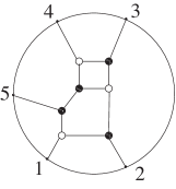
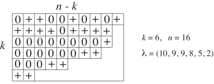
Figure 2. A plabic graph, and an irreducible Le-diagram $L=(\lambda,D)_{k,n}$.

Definition 2.9.

Fix $k$ and $n$. Let $Y_{\lambda}$ denote the Young diagram of the partition $\lambda$. A $\Gamma$ -diagram (or Le-diagram) $L=(\lambda,D)_{k,n}$ of type $(k,n)$ is a Young diagram $Y_{\lambda}$ contained in a $k\times(n-k)$ rectangle together with a filling $D:Y_{\lambda}\to\{0,+\}$ which has the $\Gamma$ -property: there is no $0$ which has a $+$ above it in the same column and a $+$ to its left in the same row. A $\Gamma$ -diagram is irreducible if each row and each column contains at least one $+$. See the right of Figure 2 for an example of an irreducible $\Gamma$ -diagram.

Theorem 2.10.

[25, Theorem 17.2] Let $S_{\mathcal{M}}^{tnn}$ be a positroid cell in $(Gr_{k,n})_{\geq 0}$. For $1\leq r\leq n$, let $I_{r}$ be the element of $\mathcal{M}$ which is lexicographically minimal with respect to the order $r<r+1<\dots<n<1<2<\dots r-1$. Then $\mathcal{I}(\mathcal{M}):=(I_{1},\dots,I_{n})$ is a Grassmann necklace of type $(k,n)$.

Lemma 2.11.

[25, Lemma 16.2] Given an irreducible Grassmann necklace $\mathcal{I}$, define a derangement $\pi=\pi(\mathcal{I})$ by requiring that: if $I_{i+1}=(I_{i}\setminus\{i\})\cup\{j\}$ for $j\neq i$, then $\pi(j)=i$. Indices are taken modulo $n$. Then $\mathcal{I}\to\pi(\mathcal{I})$ is a bijection from irreducible Grassmann necklaces $\mathcal{I}=(I_{1},\dots,I_{n})$ of type $(k,n)$ to derangements $\pi(\mathcal{I})\in S_{n}$ with $k$ excedances. The excedances of $\pi(\mathcal{I})$ are in positions $I_{1}$.

Example 2.12.

If $\mathcal{I}$ and $\pi$ are defined as in Examples 2.4 and 2.7, then $\pi(\mathcal{I})=\pi$.

Definition 2.13.

Given a $\Gamma$ -diagram $L$ contained in a $k\times(n-k)$ rectangle, label its southeast border with the numbers $1,2,\dots,n$, starting at the northeast corner. Replace each $+$ with an “elbow” and each $0$ with a “cross”; see Figure 3. Now travel along each “pipe” from southeast to northwest, and label the end of a pipe with the same number that labeled its origin. Finally, we define a permutation $\pi=\pi(L)$ as follows. If $i$ is the label of a vertical edge on the southeast border of $L$, then set $\pi(i)$ equal to the label of the vertical edge on the other side of that row. If $i$ is the label of a horizontal edge on the southeast border of $L$, then set $\pi(i)$ equal to the label of the horizontal edge on the opposite side of that column. See Figure 3.

Figure 3. The Le-diagram $L$ together with the computation of $\pi(L)=(7,4,2,9,1,3,8,6,5)$.

Proposition 2.14.

The map defined above gives a bijection from irreducible $\Gamma$ -diagrams contained in a $k\times(n-k)$ rectangle to derangements on $n$ letters with $k$ excedances.

Proof. This map can be shown to coincide with that from [30, Section 2], and up to a convention change, coincides with the map in [25, Corollary 20.1].        

Remark 2.15.

Consider a positroid cell $S_{\mathcal{M}}^{tnn}$, and suppose that the Grassmann necklace $\mathcal{I}$, the derangement $\pi$, and the $\Gamma$ -diagram $L$, satisfy $\mathcal{I}=\mathcal{I}(\mathcal{M})$, and $\pi=\pi(\mathcal{I})=\pi(L)$. Then we also refer to this cell as $S_{\mathcal{M}(\mathcal{I})}^{tnn}$, $S_{\mathcal{M}(L)}^{tnn}$, $S_{\mathcal{I}}^{tnn},S_{\pi}^{tnn}$, $S_{L}^{tnn}$, etc.

3. Soliton solutions to the KP equation

In this section we explain how to construct a $\tau$-function $\tau_{A}(x,y,{\bf t})$ from a point of $Gr_{k,n}$, and then how to obtain a soliton solution to the KP equation from that $\tau$-function.

3.1. From a point of the Grassmannian to a $\tau$-function.

We first give a realization of $Gr_{k,n}$ with a specific basis of $\mathbb{R}^{n}$. The purpose of making this non-standard choice of basis is to identify the Plücker embedding of a point $A$ of the Grassmannian with a particular $\tau$-function, in (3.5) below.

Choose real parameters $\kappa_{i}$ such that $\kappa_{1}~{}<~{}\kappa_{2}~{}\cdots~{}<\kappa_{n}$. In this paper we will assume that the $\kappa_{i}$’s are generic, meaning that:

• the sums $\mathop{\textstyle\sum}\limits_{j=1}^{p}\kappa_{i_{j}}$ are all distinct for any $p$ with $1<p<n$.

We define a set of vectors $\{\mathsf{E}_{j}^{\bf 0}:j=1,\ldots,n\}$ by

(3.1) $$\mathsf{E}_{j}^{\bf 0}:=\begin{pmatrix}1\\ \kappa_{j}\\ \vdots\\ \kappa_{j}^{n}\end{pmatrix}\,\in\,\mathbb{R}^{n}.$$

Since all $\kappa_{j}$’s are distinct, the set $\{\mathsf{E}_{j}^{\bf 0}:j=1,\ldots,n\}$ forms a basis of $\mathbb{R}^{n}$. Now define an $n\times n$ matrix $E^{\bf 0}=(\mathsf{E}_{1}^{\rm 0},\ldots,\mathsf{E}_{n}^{\bf 0})$ which is the Vandermonde matrix in the $\kappa_{j}$’s, and let $A$ be a full-rank $k\times n$ matrix representing a point of $Gr_{k,n}$. Then the vectors $\{\mathsf{F}_{i}^{\bf 0}\in\mathbb{R}^{n}:i=1,\ldots,k\}$ span a $k$-dimensional subspace in $\mathbb{R}^{n}$, where $\mathsf{F}_{i}^{\bf 0}$ is defined by

$$\mathsf{F}_{i}^{\bf 0}:=\mathop{\textstyle\sum}\limits_{j=1}^{n}a_{i,j}\,\mathsf{E}_{j}^{\bf 0},\qquad{\rm or}\qquad(\mathsf{F}_{1}^{\bf 0},\ldots,\mathsf{F}_{k}^{\bf 0})={E}^{\bf 0}A^{T},$$

where $A^{T}$ is the transpose of $A$. For $I=\{i_{1},\ldots,i_{k}\}$, define the vector $\mathsf{E}_{I}^{\bf 0}=\mathsf{E}_{i_{1}}^{\bf 0}\wedge\cdots\wedge\mathsf{E}_{i_{k}}^{\bf 0}$. Then we have a realization of the Plücker embedding:

$$\mathsf{F}_{1}^{\bf 0}\wedge\cdots\wedge\mathsf{F}_{k}^{\bf 0}=\mathop{\textstyle\sum}\limits_{I\in\binom{[n]}{k}}\Delta_{I}(A)\mathsf{E}_{I}^{\bf 0}.$$

In [27], Sato showed that each solution of the KP equation is given by a $\text{GL}_{\infty}$-orbit on the universal Grassmannian. To construct such an orbit for a finite dimensional Grassmannian, we first define multi-time variables $\hat{\bf t}:=(t_{1},\ldots,t_{m})$ for $m\geq 3$ which give a parameterization of the orbit. Then we consider a deformation $\mathsf{E}_{j}^{\hat{\bf t}}$ of the vector $\mathsf{E}_{j}^{\bf 0}$ for $j=1,\ldots,n$, given by

$$\mathsf{E}_{j}^{\hat{\bf t}}:=\mathsf{E}_{j}^{\bf 0}\exp\theta_{j}(\hat{\bf t})\qquad\text{with}\qquad\theta_{j}(\hat{\bf t}):=\mathop{\textstyle\sum}\limits_{i=1}^{m}\kappa_{j}^{i}t_{i}.$$

For the KP equation, we identify $t_{1}=x,t_{2}=y$ and $t_{3}=t$, and denote those flow parameters by

$$\hat{\mathbf{t}}=(x,y,\mathbf{t}),\qquad\text{with}\qquad\mathbf{t}:=(t_{3},\ldots,t_{m}).$$

We now define an orbit generated by the matrix $E^{\hat{\bf t}}=(\mathsf{E}_{1}^{\hat{\bf t}},\ldots,\mathsf{E}_{n}^{\hat{\bf t}})$ on elements of $\operatorname{GL}_{n}$,

$$g^{\hat{\bf t}}:=E^{\hat{\bf t}}g\qquad{\rm for~{}each}\quad g\in\operatorname{GL}_{n}.$$

Here we identify the $n\times k$ matrix consisting of the first $k$ columns of $g$ with the matrix $A^{T}$, the transpose of the matrix $A$ parametrizing a point $Gr_{k,n}$. Then the Plücker embedding gives

$$g\cdot e_{1}\wedge\cdots\wedge e_{k}=\mathop{\textstyle\sum}\limits_{1\leq i_{1}<\cdots<i_{k}\leq n}\Delta_{I}(A)\,e_{i_{1}}\wedge\cdots\wedge e_{i_{k}}.$$

where $e_{j}$ is the $j$-th standard vector in $\mathbb{R}^{n}$. Then $g^{\bf t}\cdot e_{1}\wedge\cdots\wedge e_{k}$ defines a flow (orbit) of the highest weight vector on the corresponding fundamental representation of ${\operatorname{GL}}_{n}$.

We now define the $\tau$-function as

(3.2) $$\tau(x,y,{\bf t}):= \langle e_{1}\wedge\cdots\wedge e_{k},~{}\mathsf{F}_{1}^{\hat{\bf t}}\wedge\cdots\wedge\mathsf{F}^{\hat{\bf t}}_{k}\rangle$$

$$= \langle e_{1}\wedge\cdots\wedge e_{k},~{}g^{\hat{\bf t}}\cdot e_{1}\wedge\cdots\wedge e_{k}\rangle,$$

where $\mathsf{F}^{\hat{\bf t}}_{j}:=g^{\hat{\bf t}}\cdot e_{j}$, and the bracket $\langle\cdot,\cdot\rangle$ is the usual inner product on the wedge product space $\bigwedge^{k}\mathbb{R}^{n}$. Given $I=\{i_{1},\ldots,i_{k}\}\subset[n]$, we let $E_{I}(\hat{\bf t})$ denote the scalar function

(3.3) $$\begin{array}[]{lll}E_{I}(x,y,{\bf t})&=\langle e_{1}\wedge\cdots\wedge e_{k},\,\mathsf{E}^{\hat{\bf t}}_{i_{1}}\wedge\cdots\wedge\mathsf{E}^{\hat{\bf t}}_{i_{k}}\rangle=\langle e_{1}\wedge\cdots\wedge e_{k},\,\mathsf{E}^{\bf 0}_{i_{1}}\wedge\cdots\wedge\mathsf{E}^{\bf 0}_{i_{k}}\rangle\,e^{\theta_{i_{1}}+\cdots+\theta_{i_{k}}}\\[4.30554pt] &=K_{I}\,\exp\Theta_{I}(x,y,{\bf t}),\end{array}$$

where $K_{I}:=\prod_{l<m}(\kappa_{i_{m}}-\kappa_{i_{l}})$, and $\Theta_{I}(x,y,{\bf t})$ is defined by

(3.4) $$\Theta_{I}(x,y,{\bf t}):=\mathop{\textstyle\sum}\limits_{j=1}^{k}(\kappa_{i_{j}}x+\kappa_{i_{j}}^{2}y)+\mathop{\textstyle\sum}\limits_{j=1}^{k}\theta_{i_{j}}({\bf t}).$$

Then the $\tau$-function can be written as a sum of exponential terms,

(3.5) $$\tau(x,y,{\bf t})=\tau_{A}(x,y,{\bf t})=\mathop{\textstyle\sum}\limits_{I\in\binom{[n]}{k}}\Delta_{I}(A)\,E_{I}(x,y,{\bf t}).$$

Remark 3.1.

We think of the right-hand side of (3.5) as giving the Plücker embedding of the Grassmannian $Gr_{k,n}$ into a wedge product space whose basis is given by the $E_{I}(x,y,{\bf t})$’s.

It follows that if $A\in(Gr_{k,n})_{\geq 0}$, then $\tau_{A}>0$ for all $(x,y,{\bf t})\in\mathbb{R}^{m}$.

Note that the $\tau$-function defined in (3.5) can be also written in the Wronskian form

(3.6) $$\tau_{A}(x,y,{\bf t})={\rm Wr}(f_{1},f_{2},\ldots,f_{k}),$$

with the scalar functions $\{f_{j}:j=1,\ldots,k\}$ given by

$$(f_{1},f_{2},\ldots,f_{k})^{T}=A\cdot(E_{1},E_{2},\ldots,E_{n})^{T},$$

where $E_{j}$ is the exponential function defined by $E_{j}:=\exp\theta_{j}(x,y,{\bf t})$.

3.2. From the $\tau$-function to solutions of the KP equation

It is well known (see [12, 4, 5, 6]) that if we set $x=t_{1},y=t_{2},t=t_{3}$ (treating the other $t_{i}$’s as constants), the $\tau$-function defined in (3.6) gives rise to a soliton solution of the KP equation (1.1), namely

(3.7) $$u_{A}(x,y,{\bf t})=2\frac{\partial^{2}}{\partial x^{2}}\ln\tau_{A}(x,y,{\bf t}).$$

The other $t_{j}$’s correspond to the flow parameters of the higher symmetries of the KP equation, and the set of the symmetries is called the KP hierarchy (see e.g. [22]).

It is easy to show that if $A\in(Gr_{k,n})_{\geq 0}$, then such a solution $u_{A}(x,y,\mathbf{t})$ is regular for all $t_{j}\in\mathbb{R}$. In the sequel to this paper [18], we show that if $u_{A}(x,y,{\bf t})$ is regular for all $x,y$ and $t=t_{3}$ (with the other $t_{i}$’s fixed constants), then $A\in(Gr_{k,n})_{\geq 0}$. (In [16, Proposition 4.1], a weaker statement was proved: if $u_{A}(x,y,\mathbf{t})$ is regular for all $t_{j}\in\mathbb{R}$, then $A\in(Gr_{k,n})_{\geq 0}$.) For this reason we are mainly interested in solutions $u_{A}(x,y,\mathbf{t})$ of the KP equation which come from points $A$ of $(Gr_{k,n})_{\geq 0}$.

4. From soliton solutions to soliton graphs

In this section we define certain tropical curves associated with soliton solutions: contour plots and asymptotic contour plots. We also define the notion of soliton graph.

4.1. Contour plots

One can visualize a solution $u_{A}(x,y,{\bf t})$ in the $xy$-plane by drawing level sets of the solution when the coordinates ${\bf t}=(t_{3},\ldots,t_{m})$ are fixed. For each $r\in\mathbb{R}$, we denote the corresponding level set by

$$C_{r}({\bf t}):=\{(x,y)\in\mathbb{R}^{2}:u_{A}(x,y,{\bf t})=r\}.$$

Figure 4 depicts both a three-dimensional image of a solution $u_{A}(x,y,{\bf t})$ for fixed ${\bf t}$, as well as multiple level sets $C_{r}$. These levels sets are lines parallel to the line of the wave peak.

Example 4.1.

We compute the soliton solution $u_{A}(x,y,{\bf t})$ associated to the $1\times 2$ matrix $A=(1~{}a)$ with $a>0$, considered as an element of $(Gr_{1,2})_{>0}$. Write $E_{1}=e^{\theta_{1}}$ and $aE_{2}=e^{\theta_{2}+\ln a}=e^{\tilde{\theta}_{2}}$. Then the $\tau$-function $\tau_{A}$ and the soliton solution $u_{A}$ are given by

$$\tau_{A}(x,y,{\bf t}) =e^{\theta_{1}}+e^{\tilde{\theta}_{2}}=2e^{\frac{1}{2}(\theta_{1}+\tilde{\theta}_{2})}\cosh\frac{1}{2}(\theta_{1}-\tilde{\theta}_{2}),\text{ and}$$

$$u_{A}(x,y,{\bf t}) =\frac{1}{2}(\kappa_{1}-\kappa_{2})^{2}{\rm sech}^{2}\frac{1}{2}(\theta_{1}-\tilde{\theta}_{2}).$$

This is a line-soliton solution, and the peak of the solution (wave crest) is given by the equation $\theta_{1}=\tilde{\theta}_{2}$, i.e.

$$x+(\kappa_{1}+\kappa_{2})y+\mathop{\textstyle\sum}\limits_{j=3}^{m}h_{j-1}(\kappa_{1},\kappa_{2})t_{j}=-\frac{1}{\kappa_{2}-\kappa_{1}}\ln a.$$

where we have used $\kappa_{2}^{j+1}-\kappa_{1}^{j+1}=(\kappa_{2}-\kappa_{1})h_{j}(\kappa_{1},\kappa_{2})$ with $h_{j}(\kappa_{1},\kappa_{2})=\mathop{\textstyle\sum}\limits_{p+q=j}\kappa_{1}^{p}\kappa_{2}^{q}$.

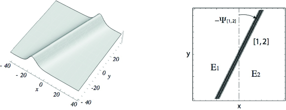
Figure 4. A line-soliton solution $u_{A}(x,y,{\bf t})$ where $A=(1,1)\in(Gr_{1,2})_{\geq 0}$, depicted via the 3-dimensional profile $u_{A}(x,y,{\bf 0})$, and the level sets of $u_{A}(x,y,0)$. $E_{i}$ represents the dominant exponential in each region.

For each fixed ${\bf t}$, $\theta_{1}=\tilde{\theta}_{2}$ gives a line which divides the $xy$-plane into two regions. The exponential $E_{1}$ dominates in the region including $x\ll 0$, and $E_{2}$ dominates the other region where $x\gg 0$. We label each region by its dominant exponential. Figure 4 depicts $u_{A}(x,y,{\bf t})$, where ${\bf t}=(0,\ldots,0)$, $a=1$, and $(\kappa_{1},\kappa_{2})=(-1,2)$.

To study the behavior of $u_{A}(x,y,\mathbf{t})$ for $A\in S_{\mathcal{M}}$, we consider the dominant exponentials at each point $(x,y,\mathbf{t})$, and we define

$$\hat{f}_{A}(x,y,\mathbf{t}) =\underset{J\in\mathcal{M}}{\max}\{\Delta_{J}(A)E_{J}(x,y,\mathbf{t})\}=\underset{J\in\mathcal{M}}{\max}\{\Delta_{J}(A)K_{J}E_{j_{1}}\dots E_{j_{k}}\}$$

$$=\underset{J\in\mathcal{M}}{\max}\biggl{\{}\exp\biggl{(}\ln\bigl{(}\Delta_{J}(A)K_{J}\bigr{)}+\Theta_{J}(x,y,{\bf t})\biggr{)}\biggr{\}},$$

where $K_{J}$ and $\Theta_{J}(x,y,{\bf t})$ are defined in (3.3) and (3.4). From (3.5), we see that $\tau_{A}$ can be approximated by $\hat{f}_{A}$.

Let $f_{A}(x,y,{\bf t})$ be the closely related function

(4.1) $${f}_{A}(x,y,{\bf t})=\underset{J\in\mathcal{M}}{\max}\left\{\ln\bigl{(}\Delta_{J}(A)K_{J}\bigr{)}+\Theta_{J}(x,y,{\bf t})\right\}.$$

Note that at a given point $(x,y,{\bf t})$, $f_{A}(x,y,{\bf t})$ is equal to a given term if and only if $\hat{f}_{A}(x,y,{\bf t})$ is equal to the exponentiated version of that term.

Definition 4.2.

Given a solution $u_{A}(x,y,{\bf t})$ of the KP equation as in (3.7), we define $\operatorname{\mathcal{C}}(u_{A},{\bf t}_{0})$ for fixed ${\bf t}={\bf t}_{0}$ to be the locus in $\mathbb{R}^{2}$ where $f_{A}(x,y,{\bf t}={\bf t}_{0})$ is not linear, and we refer to this as a contour plot of the solution $u_{A}(x,y,{\bf t})$.

4.2. Asymptotic contour plots

Some of this paper will be concerned with the contour plots for large scales of the variables $(x,y,t_{3},\ldots,t_{m})$. In this case, each of the constant terms $\ln\bigl{(}\Delta_{J}(A)K_{J}\bigr{)}$ in $f_{A}(x,y,{\bf t})$ is negligible. More precisely, we use rescaled variables $\bar{\bf t}:=(\bar{x},\bar{y},\mathbf{a})$ defined by

$$\hat{{\bf t}}=(x,y,\mathbf{t})=s\,(\bar{x},\bar{y},\mathbf{a}),\qquad\text{for some}\quad s\gg 0.$$

We then approximate $f_{A}$ by the function

$$f_{\mathcal{M}}(\bar{x},\bar{y},\mathbf{a}):=\underset{J\in\mathcal{M}}{\max}\left\{\Theta_{J}(\bar{x},\bar{y},\mathbf{a}))\right\},$$

which is obtained by taking the limit of $\frac{1}{s}f_{A}(x,y,{\bf t})$ as $s\to\infty$.

Definition 4.3.

We define the asymptotic contour plot $\operatorname{\mathcal{C}}_{{\bf a}_{0}}(\mathcal{M})$ for fixed ${\bf a}={\bf a}_{0}$ to be the locus in $\mathbb{R}^{2}$ where $f_{\mathcal{M}}(\bar{x},\bar{y},{\bf a}={\bf a}_{0})$ is not linear. Most of this paper will be concerned with the asymptotic contour plots $\operatorname{\mathcal{C}}_{{\bf a}_{0}}(\mathcal{M})$ for ${\bf a}_{0}=\pm(1,0,0,\dots)$, which we denote by $\mathcal{C}_{\pm}(\mathcal{M})$. These asymptotic contour plots are the limits of the finite contour plots $\operatorname{\mathcal{C}}(u_{A},{\bf t}_{0})$ for $A\in S_{\mathcal{M}}$ and $\hat{{\bf t}}=s\bar{{\bf t}}$ in the limit $s\to\infty$.

Note that each region of the complement of $\operatorname{\mathcal{C}}(u_{A},{\bf t}_{0})$ is a domain of linearity for $f_{A}(x,y,{\bf t}_{0})$, and hence each region is naturally associated to a dominant exponential $\Delta_{J}(A)E_{J}(x,y,{\bf t}_{0})$ from the $\tau$-function (3.5). We label this region by $E_{J}$ or $\Theta_{J}$. We label regions of the complement of each asymptotic contour plot in the same way.

A line-soliton is a finite or unbounded line segment in a contour plot (or asymptotic contour plot) which represents a balance between two dominant exponentials in the $\tau$-function. Lemma 4.4 and (4.2) provide the equation for a line-soliton.

Each contour plot $\operatorname{\mathcal{C}}(u_{A},{\bf t}_{0})$ and each asymptotic contour plot $\operatorname{\mathcal{C}}_{{\bf a}_{0}}(\mathcal{M})$ consists of line segments, some of which have finite length, while others are unbounded and extend in the $y$ direction to $\pm\infty$. The unbounded lines are all line-solitons, which we call unbounded line-solitons. The finite line segments in asymptotic contour plots are all line-solitons, but some of the finite line segments in non-asymptotic contour plots may represent phase shifts, which have lengths which are determined by the $\kappa$-parameters (see [6, page 35] for details).

Lemma 4.4.

[6, Proposition 5] Consider a line-soliton in a contour plot. The index sets of the dominant exponentials of the $\tau$-function in adjacent regions of the contour plot in the $xy$-plane are of the form $\{i,m_{2},\dots,m_{k}\}$ and $\{j,m_{2},\dots,m_{k}\}$.

According to Lemma 4.4, those two exponential terms have $k-1$ common phases, so we call the line separating them a line-soliton of type $[i,j]$, or simply an $[i,j]$-soliton. Locally we have

$$\tau_{A}\approx\Delta_{I}(A)E_{I}+\Delta_{J}(A)E_{J} =\left(\Delta_{I}(A)K_{I}E_{i}+\Delta_{J}(A)K_{J}E_{j}\right)\prod_{l=2}^{k}E_{m_{l}}$$

$$=\left(e^{\theta_{i}+\ln(\Delta_{I}(A)K_{I})}+e^{\theta_{j}+\ln(\Delta_{J}(A)K_{J}}\right)\prod_{l=2}^{k}E_{m_{l}},$$

so the equation for this line-soliton is

(4.2) $$x+(\kappa_{i}+\kappa_{j})y+\mathop{\textstyle\sum}\limits_{p=3}^{m}h_{p-1}(\kappa_{i},\kappa_{j})t_{p}=-\frac{1}{\kappa_{j}-\kappa_{i}}\ln\frac{\Delta_{J}(A)K_{J}}{\Delta_{I}(A)K_{I}}.$$

See also Example 4.1.

The equation for a line-soliton in an asymptotic contour plot is the same as in (4.2), except that the constant term on the right-hand side is $0$ (this is immediate from the definition of asymptotic contour plot).

Remark 4.5.

Consider a line-soliton given by (4.2) for fixed ${\bf t}=(t_{3},\ldots,t_{m})$. Compute the angle $\Psi_{[i,j]}$ between the line-soliton of type $[i,j]$ and the positive $y$-axis, measured in the counterclockwise direction, so that the negative $x$-axis has an angle of $\frac{\pi}{2}$ and the positive $x$-axis has an angle of $-\frac{\pi}{2}$. Then $\tan\Psi_{[i,j]}=\kappa_{i}+\kappa_{j}$, so we refer to $\kappa_{i}+\kappa_{j}$ as the slope of the $[i,j]$ line-soliton (see Figure 4). Also note that the location of the line depends on the ratio of the Plücker coordinates corresponding to the dominant exponentials on either side of the line-soliton.

We will be interested in the combinatorial structure of asymptotic contour plots, that is, the pattern of how line-solitons interact with each other. Generically we expect a point at which several line-solitons meet to have degree $3$; we regard such a point as a trivalent vertex. Three line-solitons meeting at a trivalent vertex exhibit a resonant interaction (this corresponds to the balancing condition for a tropical curve), see Section 4.4. One may also have two line-solitons which cross over each other, forming an $X$-shape: we call this an $X$-crossing, but do not regard it as a vertex. See Figure 5 for examples. We will give more details about X-crossings in Section 9.

Definition 4.6.

A contour plot $\operatorname{\mathcal{C}}(u_{A},{\bf t})$ is called generic if there exists an $\epsilon>0$ such that $\operatorname{\mathcal{C}}(u_{A},{\bf t}^{\prime})$ has the same topology as $\operatorname{\mathcal{C}}(u_{A},{\bf t})$ for any ${\bf t}^{\prime}$ satisfying $\|{\bf t}-{\bf t}^{\prime}\|<\epsilon$. Similarly, an asymptotic contour plot $\operatorname{\mathcal{C}}_{\bf a}(\operatorname{\mathcal{M}})$ is called generic if there exists an $\epsilon>0$ such that $\operatorname{\mathcal{C}}_{{\bf a}^{\prime}}(\operatorname{\mathcal{M}})$ has the same topology as $\operatorname{\mathcal{C}}_{\bf a}(\operatorname{\mathcal{M}})$ for any ${\bf a}^{\prime}$ satisfying $\|{\bf a}-{\bf a}^{\prime}\|<\epsilon$. Here the norm $\|\cdot\|$ is the usual Euclidian norm in $\mathbb{R}^{m-2}$.

4.3. Soliton graphs

The following notion of soliton graph forgets the metric data of the asymptotic contour plot, but preserves the data of how line-solitons interact and which exponentials dominate.

Definition 4.7.

Let $\operatorname{\mathcal{C}}_{{\bf a}_{0}}(\mathcal{M})$ be an asymptotic contour plot with $n$ unbounded line-solitons. Color a trivalent vertex black (respectively, white) if it has a unique edge extending downwards (respectively, upwards) from it. Label a region by $E_{I}$ if the dominant exponential in that region is $\Delta_{I}E_{I}$. Label each edge (line-soliton) by the type $[i,j]$ of that line-soliton. Preserve the topology of the metric graph, but forget the metric structure. Embed the resulting graph with bicolored vertices into a disk with $n$ boundary vertices, replacing each unbounded line-soliton with an edge that ends at a boundary vertex. We call this labeled graph the soliton graph $G_{{\bf a}_{0}}(\mathcal{M})$.

Abusing notation, we will often refer to the edges of $G_{{\bf a}_{0}}(\mathcal{M})$ as line-solitons, and use the terminology unbounded line-solitons and unbounded regions to refer to the edges and regions incident to the boundary of the disk.

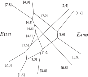
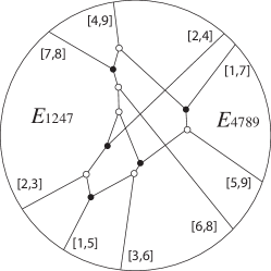
Figure 5. Example of an asymptotic contour plot and the soliton graph associated to ${\mathcal{S}}_{\pi}^{tnn}$ with $\pi=(7,4,2,9,1,3,8,6,5)$.

See Figure 5 for an example of a soliton graph. Although we have not labeled all regions or all edges, the remaining labels can be determined using Lemma 4.4.

4.4. Resonance of line-solitons

In this section we explain the physical meaning of trivalent vertices in the contour plot. It follows from Example 4.1 that a line-soliton of $[i,j]$-type has the form

$$u=\frac{1}{2}(\kappa_{i}-\kappa_{j})^{2}{\rm sech}^{2}\frac{1}{2}\Theta_{[i,j]}(x,y,{\bf t}),$$

where the phase function $\Theta_{[i,j]}(x,y,{\bf t})$ is given by

$$\Theta_{[i,j]}(x,y,{\bf t})=(\kappa_{j}-\kappa_{i})x+(\kappa_{j}^{2}-\kappa_{i}^{2})y+\mathop{\textstyle\sum}\limits_{s=3}^{m}\Omega^{(s)}_{[i,j]}(\kappa)t_{s}+\Theta_{[i,j]}^{0}(\kappa,A),$$

with

$$\Omega_{[i,j]}^{(s)}(\kappa):=\kappa_{j}^{s}-\kappa_{i}^{s},\qquad\text{and}\qquad\Theta_{[i,j]}^{0}(\kappa,A):=\ln\frac{\Delta_{J}(A)K_{J}}{\Delta_{I}(A)K_{I}}.$$

In particular, the coefficients of $x,y$ and $t=t_{3}$ are called the wavenumber-vector and the frequency, and they are given by

(4.3) $${\bf K}_{[i,j]}:=(K_{[i,j]}^{x},K_{[i,j]}^{y})=(\kappa_{j}-\kappa_{i},\kappa_{j}^{2}-\kappa_{i}^{2}),\qquad\Omega_{[i,j]}=\kappa_{j}^{3}-\kappa_{i}^{3}.$$

There is an algebraic relation, called the dispersion relation of the KP equation, among ${\bf K}_{[i,j]}$ and $\Omega_{[i,j]}$, which is given by

(4.4) $$D({\bf K}_{[i,j]},\Omega_{[i,j]}):=-4\Omega_{[i,j]}K^{x}_{[i,j]}+(K_{[i,j]}^{x})^{4}+3(K^{y}_{[i,j]})^{2}=0.$$

See [32, Chapter 11.1] for more details. This implies that if a plane wave of the form $\phi({\bf K}_{j}\cdot{\bf x}+\Omega_{j}t)$ is a solution of the KP equation, then ${\bf K}_{j}$ and $\Omega_{j}$ must satisfy the dispersion relation. Note that the wavenumber-vectors and the frequency given in (4.3) satisfy (4.4), i.e. $D({\bf K}_{j},\Omega_{j})=0$.

In wave theory, if for two plane waves $\phi_{i}({\bf K}_{i}\cdot{\bf x}+\Omega_{i}t)$ for $i=1$ and $2$ we have

$$D({\bf K}_{1}+{\bf K}_{2},\Omega_{1}+\Omega_{2})=0,$$

then as a result, a third wave can be generated. Moreover, the new wave $\phi_{3}({\bf K}_{3}\cdot\mathbf{x}+\Omega_{3}t)$ satisfies the so-called resonant conditions,

$${\bf K}_{3}={\bf K}_{1}+{\bf K}_{2},\qquad{\rm and}\qquad\Omega_{3}=\Omega_{1}+\Omega_{2}.$$

In the KP dispersion relation, the line-solitons of types $[i,j]$, $[j,\ell]$, and $[i,\ell]$ (here $i<j<\ell$) trivially satisfy the resonant conditions, i.e.

(4.5) $${\bf K}_{[i,\ell]}={\bf K}_{[i,j]}+{\bf K}_{[j,\ell]},\qquad{\rm and}\qquad\Omega_{[i,\ell]}=\Omega_{[i,j]}+\Omega_{[j,\ell]}.$$

The resonant relations (4.5) also hold for the higher terms $\Omega_{[i,j]}^{(s)}$ for $s=4,\ldots,m$, i.e.

$$\Omega_{[i,\ell]}^{(s)}=\Omega_{[i,j]}^{(s)}+\Omega_{[j,\ell]}^{(s)}\qquad\text{for}\quad s=4,\ldots,m.$$

This means that resonant interactions arise quite naturally in the KP hierarchy, and each 3-wave resonant interaction appears as a trivalent vertex in the contour plot. At that trivalent vertex, since the slope of each soliton is given by $\tan\Psi_{[i,j]}=\kappa_{i}+\kappa_{j}$, those three solitons appear as $[i,j],[j,l]$ and $[i,l]$ in counterclockwise order. This condition led us to discover a new characterization of reduced plabic graphs, which we describe in Section 10. Note also that in the contour plot, one may interpret equation (4.5) as the balancing condition for a tropical curve.

5. Permutations and soliton asymptotics

Given a contour plot $\operatorname{\mathcal{C}}(u_{A},{\bf t}_{0})$ where $A$ belongs to an irreducible positroid cell, we show that the labels of the unbounded solitons allow us to determine which positroid cell $A$ belongs to. Conversely, given $A$ in the irreducible positroid cell $S_{\pi}^{tnn}$, we can predict the asymptotic behavior of the unbounded solitons in $C(u_{A},{\bf t}_{0})$.

Theorem 5.1.

Suppose $A$ is an element of an irreducible positroid cell in $(Gr_{k,n})_{\geq 0}$. Consider the contour plot $\operatorname{\mathcal{C}}(u_{A},{\bf t}_{0})$ for any time ${\bf t}_{0}$. Then there are $k$ unbounded line-solitons at $y\gg 0$ which are labeled by pairs $[e_{r},j_{r}]$ with $e_{r}<j_{r}$, and there are $n-k$ unbounded line-solitons at $y\ll 0$ which are labeled by pairs $[i_{r},g_{r}]$ with $i_{r}<g_{r}$. We obtain a derangement in $S_{n}$ with $k$ excedances by setting $\pi(e_{r})=j_{r}$ and $\pi(g_{r})=i_{r}$. Moreover, $A$ must belong to the cell $S_{\pi}^{tnn}$.

The first part of this theorem follows from work of Biondini and Chakravarty [2, Lemma 3.4 and Theorem 3.6] (see Proposition 5.2 below) and Chakravarty and Kodama [4, Prop. 2.6 and 2.9], [6, Theorem 5] (see Theorem 5.3 below). In particular, Chakravarty and Kodama had already associated a derangement $\pi$ to $A$, but it was not clear how this $\pi$ was related to the derangement indexing the cell containing $A$. Our contribution is a proof that the derangement $\pi$ is precisely the derangement labeling the cell $S_{\pi}^{tnn}$ that $A$ belongs to (see Proposition 5.4). This fact is the first step towards establishing that various other combinatorial objects in bijection with positroid cells (Grassmann necklaces, plabic graphs) carry useful information about the corresponding soliton solutions.

Given a matrix $A$ with $n$ columns, let $A(k,\dots,\ell)$ be the submatrix of $A$ obtained from columns $k,k+1,\dots,\ell-1,\ell$, where the columns are listed in the circular order $k,k+1,\dots,n-1,n,1,2,\dots,k-1$.

Proposition 5.2.

[2, Lemma 3.4] Let $A$ be a $k\times n$ matrix representing an element in an irreducible positroid cell in $(Gr_{k,n})_{\geq 0}$, and consider the contour plot $\operatorname{\mathcal{C}}(u_{A},{\bf t}_{0})$ for any time ${\bf t}_{0}$. Then there are $n-k$ unbounded line-solitons at $y\ll 0$ and $k$ unbounded line-solitons at $y\gg 0$:

There is an unbounded line-soliton of $\operatorname{\mathcal{C}}(u_{A},{\bf t}_{0})$ at $y\ll 0$ labeled $[i,g]$ with $i<g$ if and only if

(5.1) $$\mathop{\rm rank}\nolimits A(i,\dots,g-1)=\mathop{\rm rank}\nolimits A(i+1,\dots,g)=\mathop{\rm rank}\nolimits A(i,\dots,g)=\mathop{\rm rank}\nolimits A(i+1,\dots,g-1)+1.$$

Moreoever, $g$ is a non-pivot column of $A$.

And there is an unbounded line-soliton of $\operatorname{\mathcal{C}}(u_{A},{\bf t}_{0})$ at $y\gg 0$ labeled $[e,j]$ with $e<j$ if and only if

(5.2) $$\mathop{\rm rank}\nolimits A(j,\dots,e-1)=\mathop{\rm rank}\nolimits A(j+1,\dots,e)=\mathop{\rm rank}\nolimits A(j,\dots,e)=\mathop{\rm rank}\nolimits A(j+1,\dots,e-1)+1.$$

Moreoever, $e$ is a pivot column of $A$.

Theorem 5.3.

[4, Prop. 2.6 and 2.9][6, Theorem 5] Consider an irreducible positroid cell $S_{\mathcal{M}}^{tnn}$ in $(Gr_{k,n})_{\geq 0}$, and let $A$ be a full rank matrix representing a point in that cell. Use the notation of Proposition 5.2. Define $\pi^{!}:=\pi^{!}(\mathcal{M})$ by setting $\pi^{!}(e):=j$ and $\pi^{!}(g):=(i)$ for each pivot $e$ and non-pivot $g$. Then $\pi^{!}$ is a derangement on $n$ letters with $k$ weak excedances.

Proposition 5.4.

Consider an irreducible positroid cell $S_{\mathcal{M}}^{tnn}=S_{\pi}^{tnn}$, where $\pi=\pi({\mathcal{I}}(\mathcal{M}))$. Then $\pi^{!}({\mathcal{M}})=\pi.$

Proof. Consider a $k\times n$ matrix $A$ representing an element in $S_{\mathcal{M}}^{tnn}$. Then all maximal minors of $A$ are non-negative, and the column indices of the non-zero minors are the subsets in $\mathcal{M}$. Let us first consider the derangement $\pi=\pi({\mathcal{I}}(\mathcal{M}))$. Let $I_{i}=\{i=x_{1},x_{2},\dots,x_{k}\}$ be the lexicographically minimal minor in $\mathcal{M}$ with respect to the total order $i<i+1<\dots<n<1<\dots<i-1$. Then $I_{i+1}=(I_{i}\setminus\{i\})\cup\{j\}$ is obtained from $I_{i}\setminus\{i\}$ by considering the column indices in the order $i+1,i+2,\dots,n,1,2,\dots,i$ and greedily choosing the earliest index $h$ such that the columns of $A$ indexed by the set $\{x_{2},\dots,x_{k}\}\cup\{h\}$ are linearly independent. Then $\pi(h)$ is defined to be $i$.

Now consider the ranks of various submatrices of $A$ obtained by selecting certain columns.

Claim 0. $\mathop{\rm rank}\nolimits A(i+1,\dots,h-1,h)=1+\mathop{\rm rank}\nolimits A(i+1,\dots,h-1)$. This claim follows from the way in which we chose $h$ above.

Claim 1. $\mathop{\rm rank}\nolimits A(i,i+1,\dots,h)=\mathop{\rm rank}\nolimits A(i,i+1,\dots,h-1)$. To prove this claim, we consider two cases. Either $x_{1}<_{i}h<_{i}x_{k}$ or $x_{1}<_{i}x_{k}<_{i}h$, where $<_{i}$ is the total order $i<i+1<\dots<n<1<\dots<i-1$. In the first case, the claim follows, because $h$ is not contained in the set $I_{i}$ but is contained in $I_{i+1}$. In the second case, $\mathop{\rm rank}\nolimits A(i,i+1,i+2,\dots,x_{k})=k$, and the index set $\{i,i+1,\dots,x_{k}\}$ is a strict subset of $\{i,i+1,\dots,h\}$, so $\mathop{\rm rank}\nolimits A(i,\dots,h)=\mathop{\rm rank}\nolimits A(i,\dots,h-1)=k$.

Now let $R=\mathop{\rm rank}\nolimits A(i+1,i+2,\dots,h-1)$. By Claim 0, $\mathop{\rm rank}\nolimits A(i+1,\dots,h)=R+1$. Therefore we have $\mathop{\rm rank}\nolimits A(i,\dots,h)\geq\mathop{\rm rank}\nolimits A(i+1,\dots,h)=R+1$. By Claim 1, $\mathop{\rm rank}\nolimits A(i,\dots,h)=\mathop{\rm rank}\nolimits A(i,\dots,h-1)$, but $\mathop{\rm rank}\nolimits A(i,\dots,h-1)\leq R+1$, so $\mathop{\rm rank}\nolimits A(i,\dots,h)\leq R+1$. We now have $\mathop{\rm rank}\nolimits A(i,\dots,h)=R+1$. But also $\mathop{\rm rank}\nolimits A(i,\dots,h-1)=\mathop{\rm rank}\nolimits A(i,\dots,h)=R+1$.

We have just shown that $\mathop{\rm rank}\nolimits A(i,i+1,\dots,h-1)=\mathop{\rm rank}\nolimits A(i+1,\dots,h-1,h)=\mathop{\rm rank}\nolimits A(i,\dots,h)=\mathop{\rm rank}\nolimits A(i+1,\dots,h-1)+1$. Comparing these rank conditions to either part of Proposition 5.2, and using Theorem 5.3, we see that $\pi^{!}(h)=i$. This shows that $\pi^{!}$ and $\pi$ coincide.        

Remark 5.5.

Proposition 5.4 is closely related to results on cyclic rank matrices from [14].

We now give a concrete algorithm for writing down the asymptotics of the soliton solutions of the KP equation.

Figure 6. Asymptotic line-solitons for $\pi=(6,7,1,2,8,3,9,4,5)$. Each $E_{ijkl}$ shows the dominant exponential in this region.

Theorem 5.6.

Fix real generic parameters $\kappa_{1}<\dots<\kappa_{n}$. Let $A$ be a point in an irreducible positroid cell $\operatorname{\mathcal{S}}_{\pi}^{tnn}$ in $(Gr_{k,n})_{\geq 0}$. (So $\pi$ has $k$ excedances.) For any ${\bf t}_{0}$, the asymptotic behavior of the contour plot $\mathcal{C}(u_{A},{\bf t}_{0})$ – its unbounded line-solitons and the dominant exponentials in its unbounded regions – can be read off from $\pi$ as follows.

• For $y\gg 0$, there is an unbounded line-soliton which we label $[i,\pi(i)]$ for each excedance $\pi(i)>i$. From left to right, list these solitons in decreasing order of the quantity $\kappa_{i}+\kappa_{\pi(i)}$.

• For $y\ll 0$, there is an unbounded line-soliton which we label $[\pi(j),j]$ for each nonexcedance $\pi(j)<j$. From left to right, list these solitons in increasing order $\kappa_{j}+\kappa_{\pi(j)}$.

• Label the unbounded region for $x\ll 0$ with the exponential $E_{i_{1},\dots,i_{k}}$, where $i_{1},\dots,i_{k}$ are the excedance positions of $\pi$.

• Use Lemma 4.4 to label the remaining unbounded regions of the contour plot.

Proof. The fact that the set of unbounded line-solitons are specified by the derangement $\pi$ comes from [6, Theorem 5, page 125] and [6, Corollary 1, page 124]. It then follows from Remark 4.5 that for sufficiently large $y$ (respectively, sufficiently small $y$), these solitons are ordered from left to right by decreasing (respectively, increasing) order of their slopes $\kappa_{i}+\kappa_{j}$.        

Example 5.7.

Consider the positroid cell corresponding to $(6,7,1,2,8,3,9,4,5)\in S_{9}$. The algorithm of Theorem 5.6 gives rise to the picture in Figure 6. Note that if one reads the dominant exponentials in counterclockwise order, starting from the region at the left, then one recovers exactly the Grassmann necklace from Examples 2.4 and 2.12. This correspondence will be generalized in Theorem 6.2.

6. Grassmann necklaces and soliton asymptotics

One particularly nice class of positroid cells is the TP or totally positive Schubert cells. A TP Schubert cell is a positroid cell $S_{L}^{tnn}$ which comes from a $\Gamma$ -diagram $L$ such that all boxes of $L$ contain a $+$. Note that the intersection of a usual Schubert cell with $(Gr_{k,n})_{\geq 0}$ is a union of positroid cells, of which the one with greatest dimension is the TP Schubert cell. When $A$ lies in a TP Schubert cell $S_{\pi}^{tnn}$, we can make another link between the soliton solution $u_{A}(x,y,{\bf t})$ and the combinatorics of $(Gr_{k,n})_{\geq 0}$. Namely, the dominant exponentials labeling the unbounded regions of the contour plot $\operatorname{\mathcal{C}}(u_{A},\mathbf{t})$ form the Grassmann necklace associated to $S_{\pi}^{tnn}$.

It is easy to verify the following lemma.

Lemma 6.1.

A positroid cell $S_{\pi}^{tnn}=S_{L}^{tnn}$ of $(Gr_{k,n})_{\geq 0}$ is a TP Schubert cell if and only if the following condition holds:
If $i_{1}<i_{2}<\dots<i_{k}$ and $j_{1}<j_{2}<\dots<j_{n-k}$ are the positions of the excedances and nonexcedances, respectively, of $\pi$, then $\pi(i_{1})=n-k+1$, $\pi(i_{2})=n-k+2$, …, $\pi(i_{k})=n$ and $\pi(j_{1})=1$, $\pi(j_{2})=2$, …, $\pi(j_{n-k})=n-k$.

We have the following result.

Theorem 6.2.

Let $A$ be an element of a TP Schubert cell ${\mathcal{S}}_{\pi}^{tnn}$, and consider the contour plot $\operatorname{\mathcal{C}}(u_{A},{\bf t}_{0})$ for an arbitrary time ${\bf t}_{0}$. Let the index sets of the dominant exponentials of the unbounded regions of $\operatorname{\mathcal{C}}(u_{A},{\bf t}_{0})$ be denoted $R_{1},\dots,R_{n}$, where $R_{1}$ labels the region at $x\ll 0$, and $R_{2},\dots,R_{n}$ label the regions in the counterclockwise direction from $R_{1}$. Then $(R_{1},\dots,R_{n})$ is a Grassmann necklace $\mathcal{I}$, and $\pi(\mathcal{I})=\pi$.

Theorem 6.2 is illustrated in Example 5.7. See also Figure 6.

Remark 6.3.

Theorem 6.2 does not hold if we replace “TP Schubert cell” by “positroid cell.” For example, the Grassmann necklace associated to the derangement $\pi=(4,3,1,2)$ is $(12,23,34,24)$. However, if $\kappa_{1}=0,\kappa_{2}=1,\kappa_{3}=1.5,\kappa_{4}=1.75$, then the corresponding sequence of dominant exponentials labeling the unbounded regions of any contour plot coming from the cell ${\mathcal{S}}_{\pi}^{tnn}$ is $(12,23,34,13)$.

Remark 6.4.

To recover a Grassmann necklace $\mathcal{I}=(I_{1},\dots,I_{n})$ from a derangement $\pi\in S_{n}$ (inverting the procedure of Lemma 2.11), we do the following:

• Set $I_{1}=\{i_{1},\dots,i_{k}\}$, the positions of the excedances of $\pi$.

• For each $r\geq 1$, set $I_{r+1}=(I_{r}\setminus\{r\})\cup\{\pi^{-1}(r)\}$.

We now prove Theorem 6.2.

Proof. Let $i_{1}<\dots<i_{k}$ be the positions of the excedances of $\pi$, and let $j_{1}<\dots<j_{n-k}$ be the positions of the nonexcedances. By Lemma 6.1, we have that $\pi(i_{1})<\pi(i_{2})<\dots<\pi(i_{k})$, and $\pi(j_{1})<\pi(j_{2})<\dots<\pi(j_{n-k})$. Define the partial order $\prec$ on pairs $(i,j)$ of integers in $\{1,2,\dots,n\}$ by setting $(i,j)\prec(i^{\prime},j^{\prime})$ if and only if $\kappa_{i}+\kappa_{j}<\kappa_{i^{\prime}}+\kappa_{j^{\prime}}$. Then the condition that $\kappa_{1}<\kappa_{2}<\dots<\kappa_{n}$ implies that $(i_{1},\pi(i_{1}))\prec(i_{2},\pi(i_{2}))\prec\dots\prec(i_{k},\pi(i_{k}))$ and $(j_{1},\pi(j_{1}))\prec\dots\prec(j_{n-k},\pi(j_{n-k}))$. Using Theorem 5.6, the asymptotic directions of the contour graph of the soliton solution are as in Figure 7.

Figure 7. Grassmann necklace $(R_{1},R_{2},\ldots,R_{n})$ in a contour plot associated to the TP Schubert cell ${\mathcal{S}}_{\pi}^{tnn}$.

From the conditions on our permutation, we must have $\pi(j_{1})=1,\pi(j_{2})=2,\dots,\pi(j_{n-k})=n-k$, and also $\pi(i_{1})=n-k+1,\pi(i_{2})=n-k+2,\dots,\pi(i_{k})=n$. Therefore the unbounded line-solitons of the contour plot of the soliton solution are labeled as $[i_{l},n-k+l]$ for $l=1,\ldots,k$ and $[m,j_{m}]$ for $m=1,\ldots,n-k$.

Claim 1. We claim that if $R_{1},\dots,R_{n}$ are the index sets of the dominant exponentials in the unbounded regions as in Figure 7, then $R_{\ell}$ contains $\ell$. Therefore by Lemma 4.4, $R_{\ell+1}$ is obtained from $R_{\ell}$ by removing $\ell$ and adding one more index not already in $R_{\ell}$. By Remark 6.4, Claim 1 implies $(R_{1},\dots,R_{n})$ is the Grassmann necklace associated to $\pi$, and therefore implies Theorem 6.2.

We first prove Claim 1 for $\ell\leq n-k+1$. Clearly $1\in R_{1}$, since $1$ is always the position of an excedance of a derangement. Suppose by induction that the claim is true up through $\ell-1$. Then

$$R_{\ell}=(((((\{i_{1},\dots,i_{k}\}\cup\{j_{1}\})\setminus\{1\})\cup\{j_{2}\})\setminus\{2\})\dots\cup\{j_{\ell_{1}}\})\setminus\{\ell_{1}\}.$$

Suppose that $\ell\notin R_{\ell}$. In steps $1$ through $\ell-1$, we have only removed the numbers $\{1,2,\dots,\ell-1\}$, and so $\ell\notin\{i_{1},\dots,i_{k}\}$. And we have only added the numbers $\{j_{1},\dots,j_{\ell-1}\}$, and so $\ell\notin\{j_{1},\dots,j_{\ell-1}\}$. Since $\ell\notin\{i_{1},\dots,i_{k}\}$, we have $\pi(\ell)<\ell$, and so $\ell\in\{j_{1},\dots,j_{n-k}\}$. Since $\ell\notin\{j_{1},\dots,j_{\ell-1}\}$, we have $\ell\in\{j_{\ell},j_{\ell+1},\dots,j_{n-k}\}$. But $1<j_{1}<j_{2}<\dots<j_{n-k}$ and so each element in $\{j_{\ell},j_{\ell+1},\dots,j_{n-k}\}$ is greater than $\ell$. This is a contradiction.

Claim 2. $R_{n-k+1}=\{\pi(i_{1}),\dots,\pi(i_{k})\}$. Note that since Claim 1 is true for $\ell\leq n-k+1$, $R_{n-k+1}$ contains an index for each excedance position $i_{r}$ such that $\pi^{-1}(i_{r})<i_{r}<\pi(i_{r})$. (These are the elements of $R_{1}$ that remain in each $R_{2},R_{3},\dots,R_{n-k+1}$.) $R_{n-k+1}$ also contains any nonexcedance position $j_{r}$ as long as it is not the case that $j_{r}=\pi^{-1}(j_{s})$ for some $s$. That is, $R_{n-k+1}$ contains any $j_{r}$ such that $\pi^{-1}(j_{r})<j_{r}$. Therefore we see that $R_{n-k+1}$ is equal to the set of values that $\pi$ takes at the excedance positions of $\pi$. This proves Claim 2.

We now prove Claim 1 for $\ell>n-k+1$. Again we use induction on $\ell$. The claim is true for $n-k+1$. Suppose that $\ell\notin R_{\ell}$ but Claim 1 is true for smaller $\ell$. Certainly $\ell\in R_{n-k+1}$. So $\ell\notin R_{\ell}$ means that $\ell$ must have been removed at some earlier step – say step $r$, for $n-k+1\leq r<\ell$. But the numbers removed at these steps were precisely the numbers $n-k+1,n-k+2,\dots,\ell-1$. This is a contradiction. This finishes the proof of Claim 1 and hence of Theorem 6.2.        

7. Soliton graphs are generalized plabic graphs

In this section we will show that we can think of soliton graphs as generalized plabic graphs. More precisely, we will associate a generalized plabic graph $Pl(C)$ to each soliton graph $C$. We then show that from $Pl(C)$ – whose only labels are on the boundary vertices – we can recover the labels of the line-solitons and dominant exponentials of $C$. The upshot is that all edge and region labels of a soliton graph $C$ may be reconstructed from a labeling of each boundary vertex of $C$ by an integer.

Definition 7.1.

A generalized plabic graph is an undirected graph $G$ drawn inside a disk with $n$ boundary vertices labeled $1,\dots,n$ placed in any order around the boundary of the disk, such that each boundary vertex $i$ is incident to a single edge. Each internal vertex is colored black or white, and edges are allowed to cross each other in an $X$-crossing (which is not considered to be a vertex).

Definition 7.2.

Fix an irreducible cell ${\mathcal{S}}_{\pi}^{tnn}$ of $(Gr_{k,n})_{\geq 0}$. To each soliton graph $C$ coming from that cell we associate a generalized plabic graph $Pl(C)$ by:

• labeling the boundary vertex incident to the edge $\{i,\pi_{i}\}$ by $\pi_{i}=\pi(i)$;

• forgetting the labels of all edges and regions.

See Figure 8 for a soliton graph $C$ (the same one from Figure 5) together with the corresponding generalized plabic graph $Pl(C)$.

Remark 7.3.

When $\pi$ indexes a TP Schubert cell in $(Gr_{k,n})_{\geq 0}$, the boundary vertices will be labeled by $1,2,\dots,n$ in counterclockwise order, with $1,2,\dots,n-k$ labeling the boundary vertices corresponding to the $y\ll 0$ part of the soliton graph.

We now generalize the notion of trip from [25, Section 13].

Definition 7.4.

Given a generalized plabic graph $G$, the trip $T_{i}$ is the directed path which starts at the boundary vertex $i$, and follows the “rules of the road”: it turns right at a black vertex, left at a white vertex, and goes straight through the $X$-crossings. Note that $T_{i}$ will also end at a boundary vertex. The trip permutation $\pi_{G}$ is the permutation such that $\pi_{G}(i)=j$ whenever $T_{i}$ ends at $j$.

We use the trips to label the edges and regions of each generalized plabic graph.

Definition 7.5.

Given a generalized plabic graph $G$ with $n$ boundary vertices, start at each boundary vertex $i$ and label every edge along trip $T_{i}$ with $i$. Such a trip divides the disk containing $G$ into two parts: the part to the left of $T_{i}$, and the part to the right. Place an $i$ in every region which is to the left of $T_{i}$. After repeating this procedure for each boundary vertex, each edge will be labeled by up to two numbers (between $1$ and $n$), and each region will be labeled by a collection of numbers. Two regions separated by an edge labeled by both $i$ and $j$ will have region labels $S$ and $(S\setminus\{i\})\cup\{j\}$. When an edge is labeled by two numbers $i<j$, we write $[i,j]$ on that edge, or $\{i,j\}$ or $\{j,i\}$ if we do not wish to specify the order of $i$ and $j$.

Theorem 7.6.

Consider a soliton graph $C$ coming from an irreducible positroid cell ${\mathcal{S}}_{\pi}^{tnn}$. Then the trip permutation associated to $Pl(C)$ is $\pi$, and by labeling edges and regions of $Pl(C)$ according to Definition 7.5, we will recover the original labels in $C$.

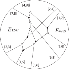
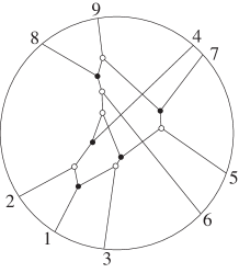
Figure 8. A soliton graph $C$ and generalized plabic graph $Pl(C)$ for $\pi=(7,4,2,9,1,3,8,6,5)$.

We invite the reader to verify Theorem 7.6 for the graphs in Figure 8.

Remark 7.7.

By Theorem 7.6, we can identify each soliton graph $C$ with its generalized plabic graph $Pl(C)$. From now on, we will often ignore the labels of edges and regions of a soliton graph, and simply record the labels on boundary vertices.

In the proof below, we will sometimes refer to the contour plot from which the soliton graph came; it is useful to think about whether edges are directed up or down.

Proof. We begin by analyzing the edge labels around a trivalent vertex in a soliton graph. They must have edge labels $[i,j]$, $[i,m]$, and $[j,m]$ in some order, where without loss of generality $i<j<m$. Recall that the slope of a line-soliton labeled $[i,j]$ is $\kappa_{i}+\kappa_{j}$. Also recall that we fixed $\kappa_{1}<\kappa_{2}<\dots<\kappa_{n}$. Therefore we know that the slopes of these three line-solitons are ordered by $\kappa_{i}+\kappa_{j}<\kappa_{i}+\kappa_{m}<\kappa_{j}+\kappa_{m}$. It follows that a trivalent vertex in the contour plot with a unique edge directed down (respectively, up) from the vertex must have line-solitons labeled as in the left (respectively, right) of Figure 9.

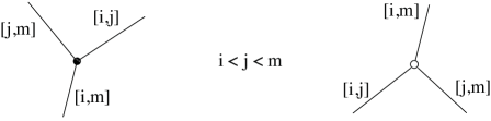
Figure 9. Contour plots of resonant interactions of three line-solitons

We now fix $r$ between $1$ and $n$, and analyze the set of all edges in the soliton graph $C$ whose label contains an $r$. We aim to show that this set of edges is a trip.

If $r$ is an excedance value of $\pi$, then we know from Theorem 5.6 that there is an edge incident to the boundary of $C$ which is labeled $[\ell,r]$, where $\ell<r$. This is an unbounded edge going to $y\to\infty$ in the contour plot. And if $r$ is a nonexcedance value, there is an edge incident to the boundary of $C$ which is labeled $[r,\ell]$ where $r<\ell$. This is an unbounded edge going to $y\to-\infty$ in the contour plot.

Considering Figure 9 and Definition 7.2, it is clear that the set of all edges containing an $r$ in $C$ will be a path between boundary vertices $r$ and $\pi_{r}$ in $Pl(C)$. We call this the soliton path.

We now claim that if we start at vertex $r$ and follow the soliton path to vertex $\pi_{r}$, then the path will have the following property: the path travels down along an edge with labels $q$ and $r$ if and only if $q<r$, and the path travels up along an edge with labels $q$ and $r$ if and only if $q>r$.

This claim is clearly true for the first edge of each soliton path. Now we just need to check that the claim remains true as we pass through black and white vertices.

Suppose that we are traveling down along an edge with labels $i$ and $r$ where $i<r$, and we get to a white vertex. Then, looking at the right side of Figure 9, we must have $m=r$, so the next edge that we traverse must be the edge $[j,m]$ in the figure (that is, $[j,r]$). Note that we will continue to go down along an edge with labels $j$ and $r$, with $j<r$.

Suppose that we are traveling down along an edge with labels $q$ and $r$ where $q<r$, and we get to a black vertex. Then, looking at the left side of Figure 9, there are two possibilities. Either we are traveling down along the left edge (labeled $[j,m]$ in the figure, so that $j=q$ and $m=r$), or we are traveling down along the right edge (labeled $[i,j]$ in the figure, so that $i=q$ and $j=r$). In the first case, the next edge we traverse will be the edge labeled $[i,m]$ in the figure, i.e. $[i,r]$, so we will continue to go down along an edge with labels $i$ and $r$, with $i<r$. In the second case, the next edge we traverse will be the edge labeled $[j,m]$ in the figure, i.e. $[r,m]$. So in this case, our next edge in the path will go up along an edge with labels $[r,m]$, where $m>r$. In all cases, the claim continues to hold.

There are also three cases to analyze if we go up along an edge. These three cases are completely analogous. Therefore the claim is true by induction.

Finally we note that in all of the above cases, every sequence of edges in the soliton path obeys the “rules of the road”. This shows that the soliton paths agree with the trips, completing the proof of Theorem 7.6.        

8. A construction for asymptotic contour plots

In this section we will explicitly compute the asymptotic contour plots $\operatorname{\mathcal{C}}_{\pm}(\mathcal{M})$. That is, we have the scaled coordinates $(\bar{x},\bar{y},{\bf a})$ with ${\bf a}=(\pm 1,0,\ldots,0)$. In particular, we will provide an algorithm that constructs the associated soliton graphs, and we will give coordinates for all the trivalent vertices in the $\bar{x}\bar{y}$-plane, which then allows one to completely describe the asymptotic contour plot. Most of this section will be devoted to the case when $a_{3}=-1$ (i.e. $t=t_{3}\to-\infty)$, and then we will explain how the same ideas can be applied to the case $a_{3}=1$ (i.e. $t=t_{3}\to\infty$).

Since we consider the coordinates $(\bar{x},\bar{y},{\bf a})=(\bar{x},\bar{y},-1,0,\ldots,0)$, we first define

$$\phi_{i}(\bar{x},\bar{y}):=\theta_{i}(x,y,-1,0,\ldots,0)=\kappa_{i}\bar{x}+\kappa_{i}^{2}\bar{y}-\kappa_{i}^{3}.$$

Then from Definition 4.3, the asymptotic contour plot $\operatorname{\mathcal{C}}_{-}(\mathcal{M})$ is defined to be the locus in $\mathbb{R}^{2}$ where

$$\underset{J\in\mathcal{M}}{\max}\left\{\mathop{\textstyle\sum}\limits_{i=1}^{k}\phi_{j_{i}}(\bar{x},\bar{y})\right\}$$

is not linear.

To compute $\mathcal{C}_{+}(\mathcal{M})$, we need to work with the functions $\phi^{\prime}_{i}(\bar{x},\bar{y}):=\theta_{i}(x,y,+1,0,\ldots,0)=\kappa_{i}\bar{x}+\kappa_{i}^{2}\bar{y}+\kappa_{i}^{3}$ instead of $\phi_{i}$. Note that $\kappa_{i}\bar{x}+\kappa_{i}^{2}\bar{y}+\kappa_{i}^{3}$ is maximized if and only if $\kappa_{i}(-\bar{x})+\kappa_{i}^{2}(-\bar{y})-\kappa_{i}^{3}$ is minimized. Therefore $\mathcal{C}_{+}(\mathcal{M})$ can be computed as the $180^{\circ}$ rotation of the locus where

$$\underset{J\in\mathcal{M}}{\min}\left\{\mathop{\textstyle\sum}\limits_{i=1}^{k}\phi_{j_{i}}(\bar{x},\bar{y})\right\}$$

is not linear.

Definition 8.1.

For $1\leq i<j\leq n$, let $L_{ij}$ be the line in the $\bar{x}\bar{y}$-plane where $\phi_{i}(\bar{x},\bar{y})=\phi_{j}(\bar{x},\bar{y})$. And let $v_{i,\ell,m}$ be the point where $\phi_{i}(\bar{x},\bar{y})=\phi_{\ell}(\bar{x},\bar{y})=\phi_{m}(\bar{x},\bar{y}).$

The following lemma is easy to check.

Lemma 8.2.

$L_{ij}$ has the equation

$$\bar{x}+(\kappa_{i}+\kappa_{j})\bar{y}-(\kappa_{i}^{2}+\kappa_{i}\kappa_{j}+\kappa_{j}^{2})=0,$$

and the points $v_{i,\ell,m}$ have coordinates

$$v_{i,\ell,m}=(-(\kappa_{i}\kappa_{\ell}+\kappa_{i}\kappa_{m}+\kappa_{\ell}\kappa_{m}),\,\kappa_{i}+\kappa_{\ell}+\kappa_{m})\in\mathbb{R}^{2}.$$

Some of the points $v_{i,\ell,m}\in\mathbb{R}^{2}$ will be trivalent vertices in the contour plots we construct; such a point corresponds to the resonant interaction of three line-solitons of types $[i,\ell]$, $[\ell,m]$ and $[i,m]$ (see Theorem 8.5 below).

8.1. Main results on $\mathcal{C}_{\pm}(\mathcal{M})$ and their soliton graphs

Consider a positroid cell $S_{\mathcal{M}}^{tnn}=S_{L}^{tnn}$ where $L$ is the $\Gamma$ -diagram indexing the cell. We will explain how to use $L$ to construct a generalized plabic graph $G_{-}(L)$.

Algorithm 8.3.

From a $\Gamma$ -diagram $L$ to the graph $G_{-}(L)$:

1. Start with a $\Gamma$ -diagram $L$ contained in a $k\times(n-k)$ rectangle, and use the construction of Definition 2.13 to replace $0$’s and $+$’s by crosses and elbows, and to label its border.

2. Add an edge, and one white and one black vertex to each elbow, as shown in the upper right of Figure 10. Forget the labels of the southeast border. If there is an endpoint of a pipe on the east or south border whose pipe starts by going straight, then erase the straight portion preceding the first elbow.

3. Forget any degree $2$ vertices, and forget any edges of the graph which end at the southeast border of the diagram. Denote the resulting graph $G_{-}(L)$.

4. After embedding the graph in a disk with $n$ boundary vertices (this is just a cosmetic change which we sometimes omit), we obtain a generalized plabic graph, which we also denote $G_{-}(L)$. If desired, stretch and rotate $G_{-}(L)$ so that the boundary vertices at the west side of the diagram are at the north instead.

Figure 10 illustrates the steps of Algorithm 8.3, starting from the $\Gamma$ -diagram of the positroid cell ${\mathcal{S}}_{\pi}^{tnn}$ where $\pi=(7,4,2,9,1,3,8,6,5)$.

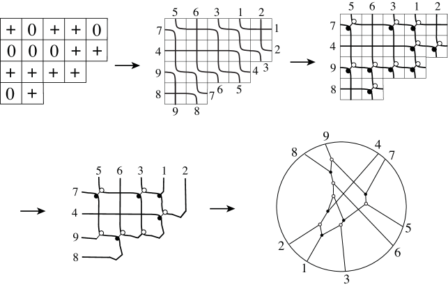
Figure 10. Construction of $G_{-}(L)$ where $\pi(L)=(7,4,2,9,1,3,8,6,5)$. The top left figure is $L$.

After labeling the edges according to the rules of the road, we will produce the graph from Figure 5.

Remark 8.4.

If every box of $L$ contains a $+$ (that is, ${\mathcal{S}}_{L}^{tnn}$ is a TP Schubert cell), then $G_{-}(L)$ will not contain any $X$-crossings.

The following is the main result of this section. The proof will be given in the next subsection.

Theorem 8.5.

Choose a positroid cell $S_{\mathcal{M}}^{tnn}=S_{L}^{tnn}=S_{\pi}^{tnn}.$ Use Algorithm 8.3 to obtain $G_{-}(L)$. Then $G_{-}(L)$ has trip permutation $\pi$, and we can use it to explicitly construct $\operatorname{\mathcal{C}}_{-}(\mathcal{M})$ as follows. Label the edges of $G_{-}(L)$ according to the rules of the road. Label each trivalent vertex incident to solitons $[i,\ell]$, $[i,m]$, and $[\ell,m]$ by $x_{i,\ell,m}$ and give that point the coordinates $(\bar{x},\bar{y})=(-(\kappa_{i}\kappa_{\ell}+\kappa_{i}\kappa_{m}+\kappa_{\ell}\kappa_{m}),\,\kappa_{i}+\kappa_{\ell}+\kappa_{m})$. Place each unbounded line-soliton of type $[i,j]$ so that it has slope $\kappa_{i}+\kappa_{j}$. (Each bounded line-soliton of type $[i,j]$ will automatically have slope $\kappa_{i}+\kappa_{j}$.)

Remark 8.6.

Although Theorem 8.5 dictates which collections of line-solitons meet at a trivalent vertex, it does not determine which pairs of line-solitons form an $X$-crossing. Which line-solitons form an $X$-crossing is determined by the parameters $(\kappa_{1},\dots,\kappa_{n})$. See Figure 11 for three contour plots based on three different choices of $(\kappa_{1},\dots,\kappa_{n})$. All of them can be constructed using the graph $G_{-}(L)$ from Figure 10, together with Theorem 8.5.

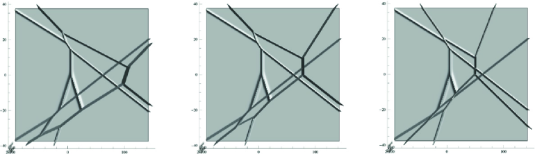
Figure 11. Three different asymptotic contour plots $\operatorname{\mathcal{C}}_{-\infty}(\operatorname{\mathcal{M}})$ where $\pi(\operatorname{\mathcal{M}})=(7,4,2,9,1,3,8,6,5)$, based on different choices for $(\kappa_{1},\dots,\kappa_{9})$. The left panel corresponds to the contour plot with $(\kappa_{1},\ldots,\kappa_{9})=(-4,-3,-2,-1,0,1,2,3,4)$; note that this is the same as $G_{-}(L)$ (cf. Figure 10).

We can use a very similar algorithm to construct $G_{+}(L)$ from the “dual” $\Gamma$ -diagram of $L$.

Definition 8.7.

Given $\mathcal{M}\subset{[n]\choose k}$, we define its dual $\mathcal{M^{*}}$ to be the collection

$$\mathcal{M^{*}}=\{\{n+1-j_{1},n+1-j_{2},\dots,n+1-j_{k}\}\ |\ \{j_{1},\dots,j_{k}\}\in\mathcal{M}\}.$$

Given $\pi\in S_{n}$, we define its dual to be the permutation $\pi^{*}=\iota\circ\pi^{-1}$, where $\iota$ is the involution in $S_{n}$ such that $\iota(j)=n+1-j$.

Given a $\Gamma$ -diagram $L$, we define its dual to be the $\Gamma$ -diagram $L^{*}$ such that $\pi(L^{*})=\pi(L)^{*}$.

Remark 8.8.

Note that which positroid cell $S_{\mathcal{M}}^{tnn}=S_{\pi}^{tnn}=S_{L}^{tnn}$ a fixed element of $(Gr_{k,n})_{\geq 0}$ lies in depends on a choice of ordered basis $(e_{1},e_{2},\dots,e_{n})$ for $\mathbb{R}^{n}$. If we relabel each basis element $e_{i}$ by $e_{n+1-i}$, then $\mathcal{M}$, $\pi$, and $L$ are replaced by their duals $\mathcal{M^{*}}$, $\pi^{*}$, and $L^{*}$.

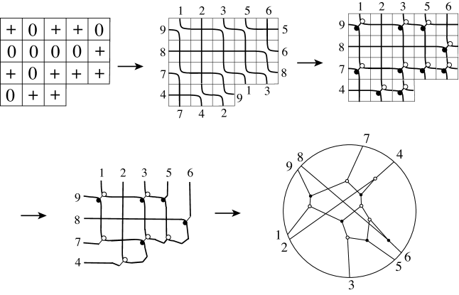
Figure 12. Construction of $G_{+}(L)$ where $\pi(L)=(7,4,2,9,1,3,8,6,5)$. The top left figure shows $L^{*}$. If we compare the unbounded solitons in $G_{+}(L)$ and $G_{-}(L)$, they appear to be in a different order. However, their order will be the same at $|y|\gg 0$.

Theorem 8.9.

Choose a positroid cell $S_{\mathcal{M}}^{tnn}=S_{L}^{tnn}=S_{\pi}^{tnn}$ where $\pi\in S_{n}$. Apply Algorithm 8.3 to $L^{*}$, but replace every label $j$ around the boundary of the $\Gamma$ -diagram and plabic graph with $\pi(n+1-j)$. This produces a graph we call $G_{+}(L)$. Then we can explicitly construct $\operatorname{\mathcal{C}}_{+}(\mathcal{M})$ from $G_{+}(L)$, just as in Theorem 8.5. See Figure 12.

8.2. The proof of Theorem 8.5

In this section we present the proof of Theorem 8.5. The main strategy is to use induction on the number of rows in the $\Gamma$ -diagram $L$. More specifically, let $L^{\prime}$ denote the $\Gamma$ -diagram $L$ with its top row removed. In Lemma 8.11 we will explain that $G_{-}(L^{\prime})$ can be seen as a labeled subgraph of $G_{-}(L)$. In Theorem 8.14, we will explain that if $\mathcal{M^{\prime}}=\mathcal{M}(L^{\prime})$, then there is a polyhedral subset of $\operatorname{\mathcal{C}}_{-}(\mathcal{M})$ which coincides with $\operatorname{\mathcal{C}}_{-}(\mathcal{M^{\prime}})$. And moreover, every vertex of $\operatorname{\mathcal{C}}_{-}(\mathcal{M^{\prime}})$ appears as a vertex of $\operatorname{\mathcal{C}}_{-}(\mathcal{M})$. By induction we can assume that Theorem 8.5 correctly computes $\operatorname{\mathcal{C}}_{-}(\mathcal{M^{\prime}})$, which in turn provides us with a description of “most” of $\operatorname{\mathcal{C}}_{-}(\mathcal{M})$, including all line-solitons and vertices whose indices do not include $1$. On the other hand, Theorem 5.6 gives a complete description of the unbounded solitons of both $\operatorname{\mathcal{C}}_{-}(\mathcal{M^{\prime}})$ and $\operatorname{\mathcal{C}}_{-}(\mathcal{M})$ in terms of $\pi(L^{\prime})$ and $\pi(L)$. In particular, $\operatorname{\mathcal{C}}_{-}(\mathcal{M})$ contains one more unbounded soliton at $\bar{y}\gg 0$ than does $\operatorname{\mathcal{C}}_{-}(\mathcal{M})$, and $\operatorname{\mathcal{C}}_{-}(\mathcal{M})$ contains $\ell$ more unbounded solitons at $\bar{y}\ll 0$ where $\ell$ is the difference in length of the first two rows. This information together with the resonance property allows us to complete the description of $\operatorname{\mathcal{C}}_{-}(\mathcal{M})$ and match it up with the combinatorics of $G_{-}(L)$.

Lemma 8.10.

Let $\pi=\pi(L)$ be the derangement associated to $L$. Then Algorithm 8.3 produces a generalized plabic graph $G_{-}(L)$ whose trip permutation is $\pi$.

Proof. It is clear from the construction that $G_{-}(L)$ is a generalized plabic graph. Note that if we follow the rules of the road starting from a boundary vertex of $G_{-}(L)$, we will first follow a “pipe” northwest (see the top right picture in Figure 10), and then travel straight across the row or column where that pipe ended. This has the same effect as the bijection of Definition 2.13.        

We now present a lemma which explains the relationship between $G_{-}(L)$ and $G_{-}(L^{\prime})$, where $L^{\prime}$ is the $\Gamma$ -diagram $L$ with the top row removed.

Lemma 8.11.

Let $L$ be a $\Gamma$ -diagram with $k$ rows and $n-k$ columns, and let $G$ denote the generalized plabic graph associated to $L$ via Algorithm 8.3. Recall that Algorithm 8.3 uses Definition 2.13 to label the boundary vertices of $G$; we then use the rules of the road to label edges of $G$ by pairs of integers. Form a new $\Gamma$ -diagram $L^{\prime}$ from $L$ by removing the top row of $L$; suppose that $\ell$ is the sum of the number of rows and columns in $L^{\prime}$. Let $G^{\prime}$ denote the edge-labeled plabic graph associated to $L^{\prime}$, but instead of using the labels $\{1,2,\dots,\ell\}$, use the labels $\{n-\ell+1,n-\ell+2,\dots,n\}$. Let $h$ denote the label of the top row of $L$. Then $G^{\prime}$ is obtained from $G$ by removing the trip $T_{h}$ starting at $h$, together with any edges to the right of the trip which have a trivalent vertex on $T_{h}$.

We omit the proof of Lemma 8.11; it should be clear after the following example.

Example 8.12.

Figure 13 illustrates Lemma 8.11 with the example of $\pi=(7,4,2,9,1,3,8,6,5)$ as in Figure 8.3. It illustrates the result of Algorithm 8.3, applied to the chain of $\Gamma$ -diagrams obtained by successively adding rows from the bottom of the diagram. We suggest that the reader use the rules of the road to fill in all edge labels on these (generalized) plabic graphs. The middle part of Figure 13 gives the permutation associated to the corresponding $\Gamma$ -diagram. Notice the relationship between the excedances in these permutations and the labeled line-solitons on the right side of the figure, e.g. the excedances $(1,2,4,7)$ and the soliton index $[1,7],[2,4],[4,9],[7,8]$ in the top figure. It follows immediately from the rules of the road that the sequence of (edge-labeled) plabic graphs on the right side of the figure are nested within each other.

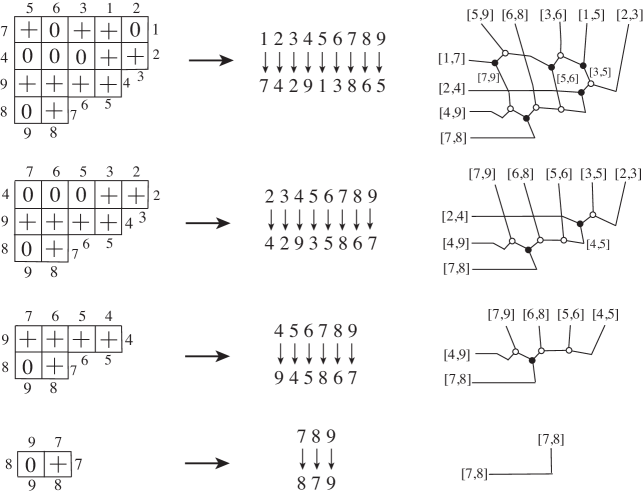
Figure 13. Inductive construction of the edge-labeled generalized plabic graph $G_{-}(L)$ of the case $\pi=(7,4,2,9,1,3,8,6,5)$.

Let $\{i_{1},\dots,i_{k}\}$ denote the lexicographically minimal element of $\mathcal{M}$. (This corresponds to the collection of pivots for any $A\in S_{\mathcal{M}}^{tnn}$.) To simplify the notation, we will assume without loss of generality that $i_{1}=1$. Now set $\mathcal{M^{\prime}}=\mathcal{M}(L^{\prime})$. We can also describe $\mathcal{M^{\prime}}=\{J\setminus\{1\}\ |\ 1\in J\text{ and }J\in\mathcal{M}\}.$ Our next goal is to explain in Theorem 8.14 the relationship between $\operatorname{\mathcal{C}}_{-}(\mathcal{M})$ and $\operatorname{\mathcal{C}}_{-}(\mathcal{M^{\prime}})$. However, we first prove a useful lemma.

Lemma 8.13.

Consider the point $v_{a,b,c}$ where $1\notin\{a,b,c\}$. Then at this point, we have that $\phi_{1}>\phi_{a}=\phi_{b}=\phi_{c}$. It follows that every region $R$ in $\operatorname{\mathcal{C}}_{-}(\mathcal{M})$ incident to the point $v_{a,b,c}$ is labeled by a dominant exponential $E_{J}$ such that $1\in J$.

Proof. Recall that $\phi_{i}(\bar{x},\bar{y})=\kappa_{i}\bar{x}+\kappa_{i}^{2}\bar{y}-\kappa_{i}^{3}.$ A calculation shows that $\phi_{a}(v_{a,b,c})=\phi_{b}(v_{a,b,c})=\phi_{c}(v_{a,b,c})=-\kappa_{a}\kappa_{b}\kappa_{c}$, while $\phi_{1}(v_{a,b,c})=-\kappa_{1}(\kappa_{a}\kappa_{b}+\kappa_{a}\kappa_{c}+\kappa_{b}\kappa_{c})+\kappa_{1}^{2}(\kappa_{a}+\kappa_{b}+\kappa_{c})-\kappa_{1}^{3}.$

Without loss of generality suppose $a<b<c$, so then $\kappa_{1}<\kappa_{a}<\kappa_{b}<\kappa_{c}$. It follows that $(\kappa_{b}-\kappa_{1})(\kappa_{c}-\kappa_{1})>0$, which implies that $\kappa_{1}\kappa_{b}+\kappa_{1}\kappa_{c}-\kappa_{1}^{2}<\kappa_{b}\kappa_{c}$. Multiplying both sides by $(\kappa_{a}-\kappa_{1})$, which is positive, we get

$$\kappa_{1}\kappa_{a}\kappa_{b}+\kappa_{1}\kappa_{a}\kappa_{c}-\kappa_{1}^{2}\kappa_{1}-\kappa_{1}^{2}\kappa_{b}-\kappa_{1}^{2}\kappa_{c}+\kappa_{1}^{3}<\kappa_{a}\kappa_{b}\kappa_{c}-\kappa_{1}\kappa_{b}\kappa_{c}.$$

Therefore

$$\kappa_{1}(\kappa_{a}\kappa_{b}+\kappa_{a}\kappa_{c}+\kappa_{b}\kappa_{c})-\kappa_{1}^{2}(\kappa_{a}+\kappa_{b}+\kappa_{c})+\kappa_{1}^{3}<\kappa_{a}\kappa_{b}\kappa_{c},$$

which implies that $\phi_{1}(v_{a,b,c})>\phi_{a}(v_{a,b,c})=\phi_{b}(v_{a,b,c})=\phi_{c}(v_{a,b,c}).$        

Theorem 8.14.

There is an unbounded polyhedral subset $\mathcal{R}$ of $\mathbb{R}^{2}$ whose boundary is formed by line-solitons of $\operatorname{\mathcal{C}}_{-}(\mathcal{M})$, such that every region in $\mathcal{R}$ is labeled by a dominant exponential $E_{J}$ for some $J$ containing $1$. In $\mathcal{R}$, $\operatorname{\mathcal{C}}_{-}(\mathcal{M})$ coincides with $\operatorname{\mathcal{C}}_{-}(\mathcal{M^{\prime}})$. Moreover, every region of $\operatorname{\mathcal{C}}_{-}(\mathcal{M^{\prime}})$ which is incident to a trivalent vertex and labeled by $E_{J^{\prime}}$ corresponds to a region of $\operatorname{\mathcal{C}}_{-}(\mathcal{M})$ which is labeled by $E_{J^{\prime}\cup\{1\}}$.

Proof. The proof of the first part of the theorem is straightforward. Note that for any value of $\bar{y}$, there is an $\bar{x}$ sufficiently large such that

$$\phi_{1}(\bar{x},\bar{y})\gg\phi_{2}(\bar{x},\bar{y})\gg\dots\gg\phi_{n}(\bar{x},\bar{y}).$$

This proves the existence of the subset $\mathcal{R}$, where every dominant exponential $E_{J}$ has the property that $1\in J$. Therefore the asymptotic contour plot within $\mathcal{R}$ depends only on the information of $\mathcal{M^{\prime}}$, and hence coincides with $\operatorname{\mathcal{C}}_{-}(\mathcal{M^{\prime}})$. (More specifically, the positions of points and line-solitons are identical, and each region label is identical to the one from $\operatorname{\mathcal{C}}_{-}(\mathcal{M^{\prime}})$ except that a $1$ is added to the index set.)

We have now shown that $\mathcal{R}$ exists, but do not yet have any information about how large it is. What we’ll show next is that $\mathcal{R}$ contains “most” of $\operatorname{\mathcal{C}}_{-}(\mathcal{M^{\prime}})$. More specifically, every region of $\operatorname{\mathcal{C}}_{-}(\mathcal{M^{\prime}})$ which is incident to at least one trivalent vertex also corresponds to a region of $\operatorname{\mathcal{C}}_{-}(\mathcal{M})$. For this we need Lemma 8.13.

By definition, all points $v_{a,b,c}$ that appear in $\operatorname{\mathcal{C}}_{-}(\mathcal{M^{\prime}})$ have the property that $1\notin\{a,b,c\}$. The three regions $R_{1}$, $R_{2}$, $R_{3}$ incident to $v_{a,b,c}$ in $\operatorname{\mathcal{C}}_{-}(\mathcal{M^{\prime}})$ are labeled by $E(J_{1})$, $E(J_{2})$, and $E(J_{3})$. In particular, this means that at region $R_{1}$, $J_{1}$ is the subset $\{j_{1},\dots,j_{k-1}\}$ of $\mathcal{M^{\prime}}$ which maximizes the value $\phi_{j_{1}}+\dots+\phi_{j_{k-1}}$. Without loss of generality we can assume that $a\in J_{1}$, $b\in J_{2}$, and $c\in J_{3}$. By Lemma 8.13, there is a neighborhood $N$ of $v_{a,b,c}$ where $\phi_{1}>\phi_{a}$. It follows that in $N\cap R_{1}$, $J_{1}\cup\{j_{k}=1\}$ is the subset of $\mathcal{M}$ that maximizes the value $\phi_{j_{1}}+\dots+\phi_{j_{k}}$. Therefore the region $R_{1}$ of $\operatorname{\mathcal{C}}_{-}(\mathcal{M^{\prime}})$ which is labeled by $E_{J_{1}}$ corresponds to a region of $\operatorname{\mathcal{C}}_{-}(\mathcal{M})$ which is labeled by $E_{J_{1}\cup\{1\}}$. Similarly for $R_{2}$ and $R_{3}$. This completes the proof of the theorem.        

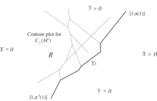
Figure 14. The asymptotic contour plot $\operatorname{\mathcal{C}}_{-}(\mathcal{M^{\prime}})$ within the asymptotic contour plot $\operatorname{\mathcal{C}}_{-}(\mathcal{M}).$

Figure 14 illustrates how the asymptotic contour plot $\operatorname{\mathcal{C}}_{-}(\mathcal{M^{\prime}})$ sits inside the asymptotic contour plot $\operatorname{\mathcal{C}}_{-}(\mathcal{M}).$ Recall that $T_{1}$ represents the trip consisting of all line-solitons labeled $[1,j]$ for any $j$ (cf. Figure 5).

Theorem 8.14 immediately implies the following.

Corollary 8.15.

The set of trivalent vertices in $\operatorname{\mathcal{C}}_{-}(\mathcal{M})$ is equal to the set of trivalent vertices in $\operatorname{\mathcal{C}}_{-}(\mathcal{M^{\prime}})$ together with some vertices of the form $v_{1,b,c}$. These vertices are the vertices along the trip $T_{1}$. In particular, every line soliton in $\operatorname{\mathcal{C}}_{-}(\mathcal{M})$ which was not present in $\operatorname{\mathcal{C}}_{-}(\mathcal{M^{\prime}})$ and is not along the trip $T_{1}$ must be unbounded. And every new bounded line-soliton in $\operatorname{\mathcal{C}}_{-}(\mathcal{M})$ that did not come from a line-soliton in $\operatorname{\mathcal{C}}_{-}(\mathcal{M^{\prime}})$ is of type $[1,j]$ for some $j$.

We can now complete the proof of Theorem 8.5. This proof will repeatedly use the characterization of unbounded line-solitons given by Theorem 5.6.

Proof. Recall that $\mathcal{M}=\mathcal{M}(L)$ and $\mathcal{M^{\prime}}=\mathcal{M}(L^{\prime})$, where $L^{\prime}$ is $L$ with the top row removed. By Theorem 8.14, we can construct the asymptotic contour plot $\operatorname{\mathcal{C}}_{-}(\mathcal{M})$ inductively from the $\Gamma$ -diagram $L$: we start by drawing the asymptotic contour plot associated with its bottom row, and then consider what happens when we add back one row at a time. On the other hand, by Lemma 8.11, the construction of Algorithm 8.3 can also be viewed as an inductive procedure which involves adding one row at a time to the $\Gamma$ -diagram. Using Lemma 8.10 and Theorem 5.6, we see that Algorithm 8.3 produces a (generalized) plabic graph whose labels on unbounded edges agree with the labels of the unbounded line-solitons for the soliton graph of any $A\in S_{L}^{tnn}$. The same is true for $A^{\prime}\in S_{L^{\prime}}^{tnn}$.

Let us now characterize the new vertices and line-solitons which $\operatorname{\mathcal{C}}_{-}(\mathcal{M})$ contains, but which $\operatorname{\mathcal{C}}_{-}(\mathcal{M^{\prime}})$ did not. In particular, we will show that the set of new vertices is precisely the set of $v_{1,b,c}$ (where $1<b<c$), such that either $c\to b$ is a nonexcedance of $\pi=\pi(\mathcal{M})$, or $c\to b$ is a nonexcedance of $\pi^{\prime}=\pi(\mathcal{M^{\prime}})$, but not both. Moreover, if $c\to b$ is a nonexcedance of $\pi$, then $v_{1,b,c}$ is white, while if $c\to b$ is a nonexcedance of $\pi^{\prime}$, then $v_{1,b,c}$ is black.

By Corollary 8.15, all new vertices have the form $v_{1,b,c}$ and lie on the trip $T_{1}$. Additionally, all new line-solitons which begin at some point $v_{1,b,c}$ and which are not on the trip $T_{1}$ must be unbounded. Since the points $v_{1,b,c}$ are trivalent, each one is incident to either an unbounded line-soliton in $\operatorname{\mathcal{C}}_{-}(\mathcal{M})$, which lies in $\mathcal{R}^{c}$, or is incident to a bounded soliton of type $[i,j]$ which lies in $\mathcal{R}$. (Possibly both are true when $i=1$).

If $v_{1,b,c}$ is incident to a bounded line-soliton $[i,j]$ which lies in $\mathcal{R}$, that soliton must have been unbounded in $\operatorname{\mathcal{C}}_{-}(\mathcal{M^{\prime}})$, and hence came from a nonexcedance $j\to i$ in $\pi^{\prime}$. (All excedances of $\pi^{\prime}$ are also excedances in $\pi$.) In particular, $i\neq 1$, so we can conclude that $v_{1,b,c}=v_{1,i,j}$. Conversely, if $j\to i$ is a nonexcedance of $\pi^{\prime}$ which is not a nonexcedance of $\pi$, then the corresponding unbounded line-soliton $[i,j]$ from $\operatorname{\mathcal{C}}_{-}(\mathcal{M^{\prime}})$ becomes a bounded line-soliton $[i,j]$ in $\operatorname{\mathcal{C}}_{-}(\mathcal{M})$ which is incident to $v_{1,i,j}$. This characterizes the new points $v_{1,b,c}$ which are incident to a bounded line-soliton $[i,j]$ contained in $\mathcal{R}$.

Each other new point $v_{1,b,c}$ will be incident to either:

• one unbounded line-soliton $[i,j]$ of $\operatorname{\mathcal{C}}_{-}(\mathcal{M})$ which lies in $\mathcal{R}^{c}$ (plus two bounded line-solitons of $T_{1}$), or

• two unbounded line-solitons of $\operatorname{\mathcal{C}}_{-}(\mathcal{M})$ which lie in $\mathcal{R}^{c}$ (plus one bounded line-soliton of $T_{1}$).

Either way, it follows that $v_{1,b,c}$ is incident to an unbounded line-soliton $[i,j]$ where $i\neq 1$, such that $j\to i$ is a nonexcedance of $\pi$ but not a nonexcedance of $\pi^{\prime}$. Therefore $v_{1,b,c}=v_{1,i,j}$.

Conversely, each nonexcedance $j\to i$ of $\pi$ (respectively, $\pi^{\prime}$) such that $1<i<j$, and such that $j\to i$ is not a nonexcedance of $\pi^{\prime}$ (respectively, $\pi$), gives rise to a point $v_{1,i,j}$ of $\operatorname{\mathcal{C}}_{-}(\mathcal{M})$. This is simply because these line-solitons must have an endpoint in $\operatorname{\mathcal{C}}_{-}(\mathcal{M})$ which did not appear in $\operatorname{\mathcal{C}}_{-}(\mathcal{M^{\prime}})$.

Also note that if $v_{1,b,c}$ is a new vertex such that $c\to b$ is a nonexcedance of $\pi$, then the line-soliton $[b,c]$ must go down (towards $\bar{y}<0$) from $v_{1,b,c}$. However, remembering the resonant condition (see Figure 9), and using the fact that $1<b<c$, we see that $[b,c]$ cannot be the only line-soliton going down from $v_{1,b,c}$. Therefore $v_{1,b,c}$ must have two line-solitons going down from it and one line-soliton going up from it, so it is a white vertex.

Similarly, if $v_{1,b,c}$ is a new vertex such that $c\to b$ is a nonexcedance of $\pi^{\prime}$, then the line-soliton $[b,c]$ must go up (towards $\bar{y}>0$) from $v_{1,b,c}$. By the resonant condition, we see that $[b,c]$ cannot be the only line-soliton going up from $v_{1,b,c}$. Therefore $v_{1,b,c}$ must have two line-solitons going up from it and one line-soliton going down from it, so it is a black vertex.

Using the bijection from Definition 2.13, it is straightforward to verify that the above description also characterizes the set of new vertices which Algorithm 8.3 associates to the top row of the $\Gamma$ -diagram $L$.

Finally, let us discuss the order in which the vertices $v_{1,b,c}$ occur along the trip $T_{1}$ in the asymptotic contour plot. First note that the trip $T_{1}$ starts at $\bar{y}<0$ and along each line-soliton it always heads up (towards $\bar{y}>0$). This follows from the resonance condition – see Figure 9 and take $i=1$. Therefore the order in which we encounter the vertices $v_{1,b,c}$ along the trip is given by the total order on the $\bar{y}$-coordinates of the vertices, namely $\kappa_{1}+\kappa_{b}+\kappa_{c}$.

We now claim that this total order is identical to the total order on the positive integers $1<b<c$, that is, it does not depend on the choice of $\kappa_{i}$’s, as long as $\kappa_{1}<\dots<\kappa_{n}$. If we can show this, then we will be done, because this is precisely the order in which the new vertices occur along the trip $T_{1}$ in the graph $G_{-}(L)$.

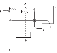
Figure 15.

To prove the claim, it is enough to show that among the set of new vertices $v_{1,b,c}$, there are not two of the form $v_{1,i,\ell}$ and $v_{1,j,k}$ where $i<j<k<\ell$. To see this, note that the indices $b$ and $c$ of the new vertices $v_{1,b,c}$ can be easily read off from the algorithm in Definition 2.13: $c$ will come from the bottom label of the corresponding column, while $b$ will come from the northwest endpoint of the pipe that $v_{1,b,c}$ lies on. Therefore, if there are two new vertices $v_{1,i,\ell}$ and $v_{1,j,k}$, then they must come from a pair of crossing pipes, as in Figure 15. Note that the crossing of the pipes must have come from a $0$ in the $\Gamma$ -diagram. From the figure it is clear that the pipe heading north from the crossing must turn west at some point, while the pipe heading west from the crossing must turn north at some point. Both of these turning points must have come from a $+$ in the $\Gamma$ -diagram, but now we see that the $\Gamma$ -diagram violates the $\Gamma$ -property. This is a contradiction, and completes the proof.        

8.3. The proof of Theorem 8.9

Theorem 8.9 can be seen as a corollary of Theorem 8.5.

Proof. Recall that $\kappa_{1}<\dots<\kappa_{n}$. We define $\lambda_{i}=-\kappa_{n+1-i}$. Then $\lambda_{1}<\dots<\lambda_{n}$. Set $\bar{y}^{\prime}=-\bar{y}$. Then

$$\underset{J\in\mathcal{M}}{\max}\left\{\mathop{\textstyle\sum}\limits_{i=1}^{k}\phi_{j_{i}}(\bar{x},\bar{y})\right\} =\underset{J\in\mathcal{M}}{\max}\left\{\mathop{\textstyle\sum}\limits_{i=1}^{k}\kappa_{j_{i}}\bar{x}+\kappa_{j_{i}}^{2}\bar{y}-\kappa_{j_{i}}^{3}\right\}$$

$$=\underset{J\in\mathcal{M}}{\min}\left\{\mathop{\textstyle\sum}\limits_{i=1}^{k}-\kappa_{j_{i}}\bar{x}-\kappa_{j_{i}}^{2}\bar{y}+\kappa_{j_{i}}^{3}\right\}$$

$$=\underset{J\in\mathcal{M}}{\min}\left\{\mathop{\textstyle\sum}\limits_{i=1}^{k}\lambda_{n+1-j_{i}}\bar{x}-\lambda_{n+1-j_{i}}^{2}\bar{y}-\lambda_{n+1-j_{i}}^{3}\right\}$$

$$=\underset{J\in\mathcal{M^{*}}}{\min}\left\{\mathop{\textstyle\sum}\limits_{i=1}^{k}\lambda_{j_{i}}\bar{x}-\lambda_{j_{i}}^{2}\bar{y}-\lambda_{j_{i}}^{3}\right\}$$

$$=\underset{J\in\mathcal{M^{*}}}{\min}\left\{\mathop{\textstyle\sum}\limits_{i=1}^{k}\lambda_{j_{i}}\bar{x}+\lambda_{j_{i}}^{2}\bar{y}^{\prime}-\lambda_{j_{i}}^{3}\right\}.$$

Therefore $\operatorname{\mathcal{C}}_{+}(\mathcal{M})$ is the locus of $\mathbb{R}^{2}$ where the last equation above is not linear. Comparing this with the definition of $\operatorname{\mathcal{C}}_{-}(\mathcal{M})$, we see that $\operatorname{\mathcal{C}}_{+}(\mathcal{M})$ can be constructed from $\operatorname{\mathcal{C}}_{-}(\mathcal{M^{*}})$, with each label $j$ replaced by $n+1-j$, and with an involution replacing $\bar{y}$ by $-\bar{y}$. The effect of the involution is to switch the colors of the black and white vertices in the plabic graph, or equivalently, to replace every boundary vertex $i$ of the plabic graph by $\pi(i)$. This completes the proof of the theorem.        

Example 8.16.

We invite readers to reconstruct the asymptotic contour plots in Figure 1. The plots correspond to the TP Schubert cell $S_{\pi}^{tnn}$ with $\pi=(4,5,1,2,6,3)$. Take the $\kappa$-parameters as $(\kappa_{1},\ldots,\kappa_{6})=(-1,-\frac{1}{2},0,\frac{1}{2},1,\frac{3}{2})$. Calculate the trivalent vertices $v_{i,j,k}=(\mp(\kappa_{i}\kappa_{j}+\kappa_{j}\kappa_{k}+\kappa_{i}\kappa_{k}),\pm(\kappa_{i}+\kappa_{j}+\kappa_{k}))$ obtained from the $\Gamma$ -diagram and its dual. There are 8 trivalent vertices for both $t\gg 0$ and $t\ll 0$ as shown in Figure 16. Then following Theorem 8.5, one obtains the asymptotic contour plots for $\operatorname{\mathcal{C}}_{\pm}(\mathcal{M})$ which approximate the plots in Figure 1.

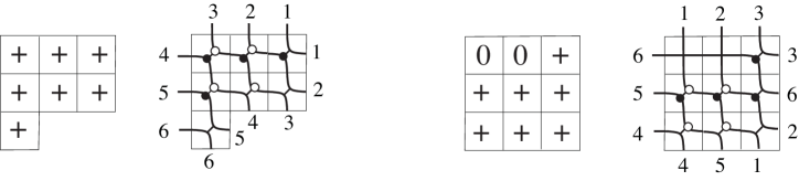
Figure 16. The Le-diagrams $L$, $L^{*}$, and the plabic graphs for $\pi=(4,5,1,2,6,3)$. Note that there are two X-crossings corresponding to the 0’s in $L^{*}$ (cf. Figure 1).

9. X-crossings and vanishing Plücker coordinates

In this section we show that for an arbitrary matroid stratum $S_{\mathcal{M}}$, and for an arbitrary vector ${\bf a}$, each $X$-crossing in the asymptotic contour plot $\operatorname{\mathcal{C}}_{{\bf a}}(\mathcal{M})$ corresponds to a vanishing Plücker coordinate, i.e. an index $J$ such that $J\notin\mathcal{M}$. This implies that for any $A\in S_{\mathcal{M}}$, the four Plücker coordinates corresponding to the dominant exponentials incident to that $X$-crossing satisfy a “two-term” Plücker relation. Note that in this section we are working over the real Grassmannian, as opposed to restricting to $(Gr_{k,n})_{\geq 0}$. One consequence of our main result (Theorem 9.1) is that the asymptotic contour plots (and hence the soliton graphs) coming from the totally positive Grassmannian $(Gr_{k,n})_{>0}$ have no $X$-crossings.

Before stating Theorem 9.1, we need some notation. Let $h_{j}(x_{1},\ldots,x_{r})$ be the complete homogeneous symmetric polynomial of degree $j$ defined by

$$h_{j}(x_{1},\ldots,x_{r})=\mathop{\textstyle\sum}\limits_{n_{1}+\cdots+n_{r}=j}x_{1}^{n_{1}}x_{2}^{n_{2}}\cdots x_{r}^{n_{r}}.$$

Then for each ${\bf a}=(a_{3},\ldots,a_{m})$, we define

(9.1) $$\gamma_{{\bf a}}(x_{1},\ldots,x_{r}):=\mathop{\textstyle\sum}\limits_{j=1}^{m-2}h_{j-1}(x_{1},\ldots,x_{r})a_{j+2},$$

Theorem 9.1.

Let $S_{\mathcal{M}}$ be a matroid stratum in $Gr_{k,n}$, and consider the corresponding asymptotic contour plot $\operatorname{\mathcal{C}}_{{\bf a}}(\mathcal{M})$ for fixed ${\bf a}$. Choose $1\leq h<i<j<\ell\leq n$, and set $\gamma_{{\bf a}}(\kappa):=\gamma_{{\bf a}}(\kappa_{h},\kappa_{i},\kappa_{j},\kappa_{\ell})$. In the statements below, $S$ is a $(k-2)$-element subset of $\{1,2,\dots,n\}$ which is disjoint from $\{h,i,j,\ell\}$.

1. Suppose there is an $X$-crossing involving line-solitons $[h,\ell]$ and $[i,j]$.

   1. Then if $\kappa_{h}+\kappa_{\ell}>\kappa_{i}+\kappa_{j}$, the dominant exponentials around the $X$-crossing in $\operatorname{\mathcal{C}}_{{\bf a}}(\mathcal{M})$ are as in Figure 17 (a). If $\gamma_{{\bf a}}(\kappa)<0$ then $S\cup\{h,\ell\}\notin\mathcal{M}$, and if $\gamma_{{\bf a}}(\kappa)>0$ then $S\cup\{i,j\}\notin\mathcal{M}$.

   2. Then if $\kappa_{i}+\kappa_{j}>\kappa_{h}+\kappa_{\ell}$, the dominant exponentials around the $X$-crossing in $\operatorname{\mathcal{C}}_{{\bf a}}(\mathcal{M})$ are as in Figure 17 (b). If $\gamma_{{\bf a}}(\kappa)<0$ then $S\cup\{i,j\}\notin\mathcal{M}$, and if $\gamma_{{\bf a}}(\kappa)>0$ then $S\cup\{h,\ell\}\notin\mathcal{M}$.

2. Suppose there is an $X$-crossing involving line-solitons $[h,i]$ and $[j,\ell]$. Then the dominant exponentials around the $X$-crossing in $\operatorname{\mathcal{C}}_{{\bf a}}(\mathcal{M})$ are as in Figure 17 (c). If $\gamma_{{\bf a}}(\kappa)<0$ then $S\cup\{j,\ell\}\notin\mathcal{M}$, and if $\gamma_{{\bf a}}(\kappa)>0$ then $S\cup\{h,i\}\notin\mathcal{M}$.

3. Suppose there is an $X$-crossing involving line-solitons $[h,j]$ and $[i,\ell]$. Then the dominant exponentials around the $X$-crossing in $\operatorname{\mathcal{C}}_{{\bf a}}(\mathcal{M})$ are as in Figure 17 (d). If $\gamma_{{\bf a}}(\kappa)<0$ then $S\cup\{h,j\}\notin\mathcal{M}$, and if $\gamma_{{\bf a}}(\kappa)>0$ then $S\cup\{i,\ell\}\notin\mathcal{M}$.

It follows that in each of the above cases, we get a “two-term” Plücker relation for any $A\in S_{\mathcal{M}}$:

• In Case (1), we have $\Delta_{i\ell S}(A)\Delta_{hjS}(A)=\Delta_{hiS}(A)\Delta_{j\ell S}(A)$.

• In Case (2), we have $\Delta_{h\ell S}(A)\Delta_{ijS}(A)=\Delta_{hjS}(A)\Delta_{i\ell S}(A).$

• In Case (3), we have $\Delta_{h\ell S}(A)\Delta_{ijS}(A)=-\Delta_{hiS}(A)\Delta_{j\ell S}(A).$

where $\Delta_{hiS}$ is shorthand for $\Delta_{\{h,i\}\cup S}$, etc.

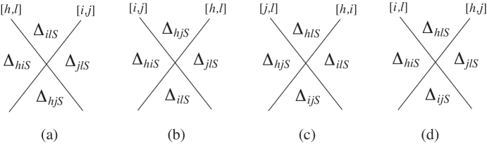
Figure 17. Different types of $X$-crossings.

Corollary 9.2 follows immediately from Theorem 9.1.

Corollary 9.2.

Let $\mathcal{M}={[n]\choose k}$ and consider the corresponding uniform matroid stratum $S_{\mathcal{M}}\subset Gr_{k,n}$. Then for any vector ${\bf a}$, there are no $X$-crossings in the asymptotic contour plot $\operatorname{\mathcal{C}}_{{\bf a}}(\mathcal{M})$. In particular, the asymptotic contour plots coming from the totally positive Grassmannian $(Gr_{k,n})_{>0}$ have no $X$-crossings.

Remark 9.3.

Note that Case (3) (i.e. Figure 17 (d)) is impossible for $A\in(Gr_{kn})_{\geq 0}$, since the relation $\Delta_{h\ell S}(A)\Delta_{ijS}(A)=-\Delta_{hiS}(A)\Delta_{j\ell S}(A)$ implies that one of these four Plücker coordinates must have a sign which is different from the other three. Therefore asymptotic contour plots associated to positroid cells cannot contain $X$-crossings involving line-solitons $[h,j]$ and $[i,\ell]$ for $h<i<j<\ell$.

9.1. Proof of Theorem 9.1

First note that if we are considering the neighborhood of an $X$-crossing formed by two line-solitons on indices ${h,i,j,\ell}$, then we may as well assume that $\{h,i,j,\ell\}=\{1,2,3,4\}$ and $S=\emptyset$.

Recall that $\kappa_{1}<\dots<\kappa_{n}$. Also recall that

$$\theta_{i}(\bar{x},\bar{y},{\bf a})=\kappa_{i}\bar{x}+\kappa_{i}^{2}\bar{y}+\mathop{\textstyle\sum}\limits_{p=3}^{m}\kappa_{i}^{p}a_{p}$$

and the asymptotic contour plot $\operatorname{\mathcal{C}}_{{\bf a}}(\mathcal{M})$ is defined to be the locus in $\mathbb{R}^{2}$ where

$$f_{\mathcal{M}}(\bar{x},\bar{y},{\bf a})=\underset{J\in\mathcal{M}}{\max}\left\{\mathop{\textstyle\sum}\limits_{i=1}^{k}\theta_{j_{i}}(\bar{x},\bar{y},{\bf a})\right\}$$

is not linear.

Recall from (4.2) that a line-soliton of type $[i,j]$ in $\operatorname{\mathcal{C}}_{{\bf a}}(\mathcal{M})$ lies on the line $L_{ij}$ whose equation is

(9.2) $$\bar{x}+(\kappa_{i}+\kappa_{j})\bar{y}+\mathop{\textstyle\sum}\limits_{p=1}^{m-2}h_{p+1}(\kappa_{i},\kappa_{j})a_{p+2}=0.$$

Lemma 9.4.

Let $\kappa_{a}<\kappa_{b}<\kappa_{c}$. Then the $\bar{y}$-coordinate of the trivalent vertex $v_{abc}=(v^{\bar{x}}_{abc},v^{\bar{y}}_{abc})$ where the lines $L_{a,b}$, $L_{b,c}$, and $L_{a,c}$ mutually intersect is given by

$$v_{abc}^{\bar{y}}=-\mathop{\textstyle\sum}\limits_{p=1}^{m-2}h_{p}(\kappa_{a},\kappa_{b},\kappa_{c})a_{p+2}.$$

Proof. From the intersection between $L_{a,b}$ and $L_{b,c}$, we have

$$(\kappa_{c}-\kappa_{a})\bar{y}+\mathop{\textstyle\sum}\limits_{p=1}^{m-2}[h_{p+1}(\kappa_{b},\kappa_{c})-h_{p+1}(\kappa_{a},\kappa_{b})]a_{p+2}=0.$$

So we need to show that

$$h_{p+1}(\kappa_{b},\kappa_{c})-h_{p+1}(\kappa_{a},\kappa_{b})=(\kappa_{c}-\kappa_{a})h_{p}(\kappa_{a},\kappa_{b},\kappa_{c}).$$

This follows from Lemma 9.5 below.        

Lemma 9.5.

For each $i\geq 1$, we have

$$h_{i}(x_{1},\ldots,x_{r},x_{\alpha})-h_{i}(x_{1},\ldots,x_{r},x_{\beta})=(x_{\alpha}-x_{\beta})h_{i-1}(x_{1},\ldots,x_{r},x_{\alpha},x_{\beta}).$$

Proof. Recall that the generating function for the homogeneous symmetric polynomials is given by

$$\exp\left[\mathop{\textstyle\sum}\limits_{i=1}^{\infty}\frac{1}{i}\left(\mathop{\textstyle\sum}\limits_{j=1}^{r}x_{j}^{i}\right)\lambda^{i}\right]=\mathop{\textstyle\sum}\limits_{i=0}^{\infty}h_{i}(x_{1},\ldots,x_{r})\lambda^{i}.$$

Then we have

$$\mathop{\textstyle\sum}\limits_{i=1}^{\infty}\left[h_{i}(x_{1},\ldots,x_{r},x_{\alpha})-h_{i}(x_{1},\ldots,x_{r},x_{\beta})\right]\lambda^{i}$$

$$= \exp\left[\mathop{\textstyle\sum}\limits_{i=1}^{\infty}\frac{1}{i}\left(\mathop{\textstyle\sum}\limits_{j=1}^{r}x_{j}^{i}+x_{\alpha}^{i}\right)\lambda^{i}\right]-\exp\left[\mathop{\textstyle\sum}\limits_{i=1}^{\infty}\frac{1}{i}\left(\mathop{\textstyle\sum}\limits_{j=1}^{r}x_{j}^{i}+x_{\beta}^{i}\right)\lambda^{i}\right]$$

$$= \exp\left[\mathop{\textstyle\sum}\limits_{i=1}^{\infty}\frac{1}{i}\left(\mathop{\textstyle\sum}\limits_{j=1}^{r}x_{j}^{i}+x_{\alpha}^{i}+x_{\beta}^{i}\right)\lambda^{i}\right]\left(e^{-\mathop{\textstyle\sum}\limits\frac{1}{i}x_{\beta}^{i}\lambda^{i}}-e^{-\mathop{\textstyle\sum}\limits\frac{1}{i}x_{\alpha}^{i}\lambda^{i}}\right)$$

$$= \left[\mathop{\textstyle\sum}\limits_{i=0}^{\infty}h_{i}(x_{1},\ldots,x_{r},x_{\alpha},x_{\beta})\lambda^{i}\right](x_{\alpha}-x_{\beta})\lambda$$

$$= (x_{\alpha}-x_{\beta})\mathop{\textstyle\sum}\limits_{i=1}^{\infty}h_{i-1}(x_{1},\ldots,x_{r},x_{\alpha},x_{\beta})\lambda^{i}.$$

Here we have used the formula

$$\mathop{\textstyle\sum}\limits_{i=1}^{\infty}\frac{1}{i}x^{i}=-\ln(1-x).$$

     

Lemma 9.6.

Recall from (9.1) and Theorem 9.1 the definition of $\gamma_{{\bf a}}(\kappa)=\gamma_{{\bf a}}(\kappa_{h},\kappa_{i},\kappa_{j},\kappa_{\ell})$. Then using Lemma 9.4, we have

• if $\gamma_{{\bf a}}(\kappa)<0$, then $v_{123}^{\bar{y}}<v_{124}^{\bar{y}}<v_{134}^{\bar{y}}<v_{234}^{\bar{y}}$, and

• if $\gamma_{{\bf a}}(\kappa)>0$, then $v_{123}^{\bar{y}}>v_{124}^{\bar{y}}>v_{134}^{\bar{y}}>v_{234}^{\bar{y}}.$

Proof. Using Lemma 9.5, we compute

$$v_{abd}^{\bar{y}}-v_{abc}^{\bar{y}} =-\mathop{\textstyle\sum}\limits_{p=1}^{m-2}\left[h_{p}(\kappa_{a},\kappa_{b},\kappa_{d})-h_{p}(\kappa_{a},\kappa_{b},\kappa_{c})\right]\,a_{p+2}$$

$$=-(\kappa_{d}-\kappa_{c})\left[\mathop{\textstyle\sum}\limits_{p=1}^{m-2}h_{p-1}(\kappa_{a},\kappa_{b},\kappa_{c},\kappa_{d})a_{p+2}\right]$$

$$=-(\kappa_{d}-\kappa_{c})\gamma_{{\bf a}}(\kappa).$$

Then it is straightforward to show the assertion.        

We have the following total order on the slopes of the lines $L_{ij}$ for $1\leq i<j\leq 4$:

• If $\kappa_{1}+\kappa_{4}>\kappa_{2}+\kappa_{3}$ then

  $$\kappa_{1}+\kappa_{2}<\kappa_{1}+\kappa_{3}<\kappa_{2}+\kappa_{3}<\kappa_{1}+\kappa_{4}<\kappa_{2}+\kappa_{4}<\kappa_{3}+\kappa_{4}.$$

• If $\kappa_{1}+\kappa_{4}<\kappa_{2}+\kappa_{3}$ then

  $$\kappa_{1}+\kappa_{2}<\kappa_{1}+\kappa_{3}<\kappa_{1}+\kappa_{4}<\kappa_{2}+\kappa_{3}<\kappa_{2}+\kappa_{4}<\kappa_{3}+\kappa_{4}.$$

Proposition 9.7.

Suppose $\gamma_{{\bf a}}(\kappa)=\gamma_{{\bf a}}(\kappa_{1},\kappa_{2},\kappa_{3},\kappa_{4})<0$. If $\kappa_{1}+\kappa_{4}>\kappa_{2}+\kappa_{3}$ then the configuration of lines $L_{ij}$ for $1\leq i<j\leq 4$ is as in the left of Figure 18 (up to perturbing the $\kappa_{i}$’s, which perturbs the slopes of lines while keeping the total order as shown above). And if $\kappa_{1}+\kappa_{4}<\kappa_{2}+\kappa_{3}$ then the configuration of lines is as in the right of Figure 18.

For the other cases with $\gamma_{{\bf a}}(\kappa)>0$, the configurations of lines $L_{ij}$ can be obtained by a $180^{\circ}$ rotation of those figures.

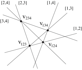
Figure 18. The configuration of the lines $L_{ij}$ for $\gamma_{{\bf a}}(\kappa)<0$, based on whether $\kappa_{1}+\kappa_{4}>\kappa_{2}+\kappa_{3}$ or $\kappa_{1}+\kappa_{4}<\kappa_{2}+\kappa_{3}$.

Proof. Let $x$ be the point where $L_{14}$ and $L_{23}$ meet. If $\kappa_{1}+\kappa_{4}>\kappa_{2}+\kappa_{3}$, then $L_{24}$ must intersect both $L_{14}$ and $L_{23}$ below $x$. This follows from the fact that $\kappa_{2}+\kappa_{4}>\kappa_{1}+\kappa_{4}$ and $v_{124}^{\bar{y}}<v_{234}^{\bar{y}}$ (from Lemma 9.6). While if $\kappa_{1}+\kappa_{4}<\kappa_{2}+\kappa_{3}$, then $L_{24}$ must intersect both $L_{14}$ and $L_{23}$ above $x$. This follows from the fact that $\kappa_{2}+\kappa_{4}>\kappa_{2}+\kappa_{3}$ and $v_{124}^{\bar{y}}<v_{234}^{\bar{y}}$. In either case, we can now draw $L_{24}$, and so have locations for the points $v_{124}$ and $v_{234}$.

Now consider the placement of $L_{13}$. If $\kappa_{1}+\kappa_{4}>\kappa_{2}+\kappa_{3}$ (respectively $\kappa_{1}+\kappa_{4}<\kappa_{2}+\kappa_{3}$) then $\kappa_{1}+\kappa_{3}<\kappa_{2}+\kappa_{3}$ (respectively, $\kappa_{1}+\kappa_{3}<\kappa_{1}+\kappa_{4}$). And $L_{13}$ intersects $L_{14}$ and $L_{23}$ in $v_{134}$ and $v_{123}$, which must satisfy $v_{234}^{\bar{y}}>v_{134}^{\bar{y}}>v_{124}^{\bar{y}}>v_{123}^{\bar{y}}$. So $L_{13}$ must be as shown in Figure 18. We now have locations for all four points $v_{ijk}$, so we can draw in all six lines $L_{ij}$.        

Now for each region in the two figures, we will compute the total order on $\{\theta_{1},\theta_{2},\theta_{3},\theta_{4}\}$. If $\theta_{a}(\bar{x},\bar{y},{\bf a})>\theta_{b}(\bar{x},\bar{y},{\bf a})>\theta_{c}(\bar{x},\bar{y},{\bf a})>\theta_{d}(\bar{x},\bar{y},{\bf a})$ then we will write $abcd$ as shorthand for this order. Also note that if $\bar{y}$ is finite then for $\bar{x}\ll 0$, we have $\theta_{1}(\bar{x},\bar{y},{\bf a})>\theta_{2}(\bar{x},\bar{y},{\bf a})>\theta_{3}(\bar{x},\bar{y},{\bf a})>\theta_{4}(\bar{x},\bar{y},{\bf a}).$ This allows us to compute the total orders on the $\theta_{i}$’s, as shown in Figure 19.

Figure 19. The total order on the $\theta_{i}(\bar{x},\bar{y},{\bf a})$’s for $\gamma_{{\bf a}}(\kappa)<0$, based on whether $\kappa_{1}+\kappa_{4}>\kappa_{2}+\kappa_{3}$ or $\kappa_{1}+\kappa_{4}<\kappa_{2}+\kappa_{3}$.

Using Figure 19 for $\gamma_{{\bf a}}(\kappa)<0$, we can compute the dominant exponentials. To compute the dominant exponentials in a given region, we consider the region label $abcd$ and choose the leftmost two indices such that the corresponding Plücker coordinate is nonzero.

We now prove Theorem 9.1.

Proof. Consider Part (1a) of the theorem. Suppose that we see an $X$-crossing in the contour plot involving line-solitons of types $[1,4]$ and $[2,3]$. Let us consider the local neighborhood of this $X$-crossing, looking at the left of Figure 19. Note that in all four regions immediately incident to the $X$-crossing, we have that each of $\theta_{1}$ and $\theta_{4}$ is greater than each of $\theta_{2}$ and $\theta_{3}$. So at $\gamma_{{\bf a}}(\kappa)<0$, if $\Delta_{14}(A)\neq 0$, then this $X$-crossing would not appear in the contour plot ($E_{14}$ would be the dominant exponential in a neighborhood of the $X$-crossing). Therefore we must have $\Delta_{14}(A)=0$.

Similarly, at $\gamma_{{\bf a}}(\kappa)>0$, if $\Delta_{23}(A)\neq 0$, then this $X$-crossing would not appear in the contour plot ($E_{23}$ would be the dominant exponential in a neighborhood of the $X$-crossing.) Therefore we must have $\Delta_{23}(A)=0$.

Proving Part (1b) of the theorem is precisely analogous, but we look at the right of Figure 19. Proving Parts (2) and (3) are very similar, and we leave them to the reader.        

10. TP Schubert cells, reduced plabic graphs, and cluster algebras

The most important plabic graphs are those which are reduced [25, Section 12]. Although it is not easy to characterize reduced plabic graphs (they are defined to be plabic graphs whose move-equivalence class contains no graph to which one can apply a reduction), they are very important because of their application to cluster algebras [29] and parameterizations of cells [25].

In this section, after recalling definitions, we will state and prove a new characterization of reduced plabic graphs. We then use this characterization to prove that soliton graphs for TP Schubert cells which have no $X$-crossings are in fact reduced plabic graphs. Using Corollary 9.2, we deduce that the set of dominant exponentials labeling any soliton graph for the TP Grassmannian is a cluster for the cluster algebra associated to the Grassmannian. We conjecture that the coordinate ring of each Schubert variety has a cluster algebra structure in which the set of dominant exponentials labeling a soliton graph without $X$-crossings for the corresponding TP Schubert cell is a cluster.

10.1. Reduced plabic graphs

We will always assume that a plabic graph is leafless, i.e. that it has no non-boundary leaves, and that it has no isolated components. In order to define reduced, we first define some local transformations of plabic graphs.

(M1) SQUARE MOVE. If a plabic graph has a square formed by four trivalent vertices whose colors alternate, then we can switch the colors of these four vertices.

Figure 20. Square move

(M2) UNICOLORED EDGE CONTRACTION/UNCONTRACTION. If a plabic graph contains an edge with two vertices of the same color, then we can contract this edge into a single vertex with the same color. We can also uncontract a vertex into an edge with vertices of the same color.

Figure 21. Unicolored edge contraction

(M3) MIDDLE VERTEX INSERTION/REMOVAL. If a plabic graph contains a vertex of degree 2, then we can remove this vertex and glue the incident edges together; on the other hand, we can always insert a vertex (of any color) in the middle of any edge.

Figure 22. Middle vertex insertion/ removal

(R1) PARALLEL EDGE REDUCTION. If a network contains two trivalent vertices of different colors connected by a pair of parallel edges, then we can remove these vertices and edges, and glue the remaining pair of edges together.

Figure 23. Parallel edge reduction

Definition 10.1.

[25] Two plabic graphs are called move-equivalent if they can be obtained from each other by moves (M1)-(M3). The move-equivalence class of a given plabic graph $G$ is the set of all plabic graphs which are move-equivalent to $G$. A leafless plabic graph without isolated components is called reduced if there is no graph in its move-equivalence class to which we can apply (R1).

Theorem 10.2.

[25, Theorem 13.4] Two reduced plabic graphs which each have $n$ boundary vertices are move-equivalent if and only if they have the same trip permutation.

10.2. A new characterization of reduced plabic graphs

Definition 10.3.

We say that a (generalized) plabic graph has the resonance property, if after labeling edges via Definition 7.5, the set $E$ of edges incident to a given vertex has the following property:

• there exist numbers $i_{1}<i_{2}<\dots<i_{m}$ such that when we read the labels of $E$, we see the labels $[i_{1},i_{2}],[i_{2},i_{3}],\dots,[i_{m-1},i_{m}],[i_{1},i_{m}]$ appear in counterclockwise order.

We call this the resonance property by analogy with the resonance of solitons (see Section 4.4).

Remark 10.4.

Note that the graphs in Figure 9 satisfy the resonance property.

Theorem 10.5.

A plabic graph is reduced if and only if it has the resonance property.

Remark 10.6.

In fact, our proof below also proves that if a generalized plabic graph has the resonance property, then it is reduced.

Proof. By Proposition 10.8 below, for every positroid cell ${\mathcal{S}}_{L}^{tnn}$ there is a reduced plabic graph $G_{L}^{\hbox{\begin{sideways}\begin{sideways}$\Gamma$\end{sideways}\end{sideways}}}$ satisfying the resonance property, whose trip permutation equals $\pi(L)$. We will show that the moves (M1), (M2), and (M3) preserve the resonance property. This will show that the entire move-equivalence class of $G_{L}$ satisfies the resonance property.

Figure 24. The edge-labeling of the square move

By consideration of the rules of the road, the edges of a plabic graph with a local configuration as in the left of Figure 20 must be labeled by the pairs of integers as shown in the left of Figure 24, for some $i,j,k,m$. The edge labeling after a square move is shown in the right of Figure 24. But now note that if we compare the top left vertex of the left figure with the bottom right vertex of the right figure, their edge labels together with the circular order on them concide. Similarly we can match the other three vertices of the left figure with the other three vertices of the right figure in Figure 24. Therefore the labels around each vertex at the left of Figure 24 satisfy the resonance property if and only if the labels around each vertex at the right of Figure 24 satisfy the resonance property.

Figure 25. The edge-labeling of the unicolored edge contraction

Similarly, the edge labels of a plabic graph with a local configuration as in the left of Figure 21 must be as in the left of Figure 25, for some integers $h,i,j,k,m$. The right of Figure 25 show the new edge labels we’d get after a unicolored edge contraction. Note that in order for the configuration on the left to satisfy the resonance property, we must have $h,i,j,k,m$ be cyclically ordered, e.g. $h<i<j<k<m$ or $i<j<k<m<h$ or $j<k<m<h<i$ or …. Similarly, in order for the configuration at the right of Figure 25 to satisfy the resonance property, we must have $h,i,j,k,m$ be cyclically ordered. Therefore the move (M2) preserves the resonance property.

The move (M3) trivially preserves the resonance property. All edges in Figure 22 will be labeled $[i,j]$ for some $i$ and $j$. Therefore we have shown that moves (M1), (M2), and (M3) preserve the resonance property.

By [25, Theorem 13.4], for any two reduced plabic graphs $G$ and $G^{\prime}$ with the same number of boundary vertices, the following claims are equivalent:

• $G$ can be obtained from $G^{\prime}$ by moves (M1)-(M3)

• $G$ and $G^{\prime}$ have the same (decorated) trip permutation.

Therefore it follows that all reduced plabic graphs with the (decorated) trip permutation $\pi$ satisfy the resonance property. Letting $L$ vary over all $\Gamma$ -diagrams, we see that all reduced plabic graphs satisfy the resonance property.

Now we need to show that if a plabic graph $G$ has the resonance property, then it must be reduced. Assume for the sake of contradiction that it is not reduced. Then by [25, Lemma 12.6], there is another graph $G^{\prime}$ in its move-equivalence class to which one can apply a parallel edge reduction (R1). Since applications of (M1), (M2), (M3) preserve the resonance property, $G^{\prime}$ has the resonance property. But then, it is impossible to apply (R1).

Figure 26. The edge-labeling of the parallel edge reduction

This is because an edge-labeling of a local configuration to which one can apply (R1) must be as in the left hand side of Figure 26. However, this local configuration violates the resonance property: it has a trivalent vertex with two incident edges which have the same edge-label. Therefore one cannot apply (R1) to $G^{\prime}$ so $G$ must be reduced.        

We now provide an algorithm from [25, Section 20] for associating a reduced plabic graph $G_{L}^{\hbox{\begin{sideways}\begin{sideways}$\Gamma$\end{sideways}\end{sideways}}}$ to any $\Gamma$ -diagram $L$. The plabic graph $G_{L}^{\hbox{\begin{sideways}\begin{sideways}$\Gamma$\end{sideways}\end{sideways}}}$ will have the trip permutation $\pi(L)$.

Algorithm 10.7.

[25, Section 20]

1. Start with a $\Gamma$ -diagram $L$ contained in a $k\times(n-k)$ rectangle, and label its southeast border from $1$ to $n$, starting from the northeast corner of the rectangle. Reflect the figure over the horizontal axis.

2. From the center of each box containing a $+$, drop a “hook” up and to the right, so that the arm and leg of the hook extend beyond the east and north boundary of the Young diagram. Consider the hook graph $H(L)$ formed by the set of all such hooks.

3. Make local modifications to $H(L)$ as in Figure 27.

   

   Figure 27.

4. The border labels from the first picture become labeled “boundary vertices;” they are labeled $1$ to $n$ in counterclockwise order. After embedding the figure in a disk, we have a plabic graph which we denote by $G_{L}^{\hbox{\begin{sideways}\begin{sideways}$\Gamma$\end{sideways}\end{sideways}}}$.

Figure 28 illustrates the steps of Algorithm 10.7.

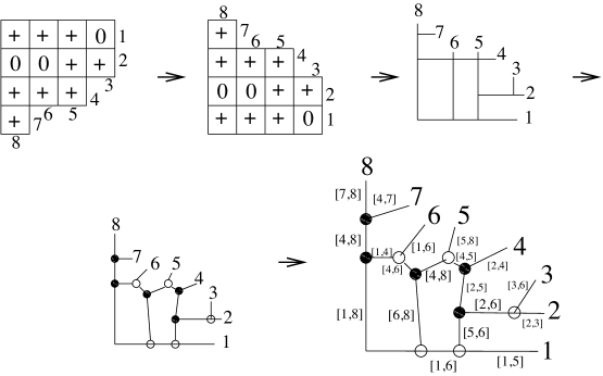
Figure 28. A plabic graph for ${\mathcal{S}}_{\pi}^{tnn}$ with $\pi=(6,4,2,7,1,3,8,5)$

Proposition 10.8.

The plabic graph $G_{L}^{\hbox{\begin{sideways}\begin{sideways}$\Gamma$\end{sideways}\end{sideways}}}$has the resonance property.

Proof. We prove this directly by analyzing the trips in the graph. One can collapse the plabic graph $G_{L}^{\hbox{\begin{sideways}\begin{sideways}$\Gamma$\end{sideways}\end{sideways}}}$ back to the hook graph $H(L)$, and consider how the trips look in $H(L)$. In $H(L)$, the trips have the following form:

• a trip which starts from the label of a vertical edge in the original $\Gamma$ -diagram first goes west as far as possible, and then takes a zigzag path north and east, turning whenever possible.

• a trip which starts from the label of a horizontal edge in the original $\Gamma$ -diagram first goes south as far as possible, and then takes a zigzag path east and north, turning whenever possible.

See Figure 29 for a depiction of the general form of the trips, as well as the trip which begins at $8$ in the example from Figure 28.

Figure 29.

We now analyze the edge labeling around a black vertex in $G_{L}^{\hbox{\begin{sideways}\begin{sideways}$\Gamma$\end{sideways}\end{sideways}}}$ which comes from a trivalent vertex in the hook graph $H(L)$, see Figure 30. By consideration of the zigzag shape of the trips, the trip which approaches the black vertex from above must come straight south from some boundary vertex labeled $j$, while the trip which approaches the black vertex from the right must come straight west from some boundary vertex $i$. The trip which approaches the black vertex from below could have started from a boundary vertex $k$ which is either southeast of $i$ or west of $j$, see the first two pictures in Figure 30. Either way, the resulting edge labeling will be as shown in the third picture in Figure 30. Clearly $i<j$, and either $k<i$ or $k>j$. Therefore the edge labeling in the third picture in Figure 30 satisfies the resonance property.

Figure 30.

The argument for a white vertex in $G_{L}^{\hbox{\begin{sideways}\begin{sideways}$\Gamma$\end{sideways}\end{sideways}}}$ which comes from a trivalent vertex in the hook graph $H(L)$ is analogous; see the fourth, fifth, and sixth pictures in Figure 30.

Finally we analyze the edge labeling around a pair of vertices in $G_{L}^{\hbox{\begin{sideways}\begin{sideways}$\Gamma$\end{sideways}\end{sideways}}}$ which came from a degree $4$ vertex in $H(L)$. In $H(L)$, the trip which approaches the vertex from above must come straight south from some boundary vertex labeled $j$, while the trip which approaches the vertex from the right must come straight west from some boundary vertex $i$. As before, $i<j$. Let $k$ and $\ell$ denote the boundary vertices whose trips approach the degree $4$ vertex from the left and below, respectively. The resulting edge-labeling is shown at the right of Figure 31.

There are multiple possibilities for the trips starting from $k$ and $\ell$; Figure 31 shows several of them. The only restriction is that neither $k$ nor $\ell$ lies in between $i$ and $j$. In particular, one of the following must be true:

• $k<i<j$ and $\ell<i<j$

• $i<j<k$ and $i<j<\ell$

• $k<i<j<\ell$

• $\ell<i<j<k$

In all cases, the edge labeling in Figure 31 satisfies the resonance property.

Figure 31.

     

Corollary 10.9.

Let $S_{\mathcal{M}}^{tnn}$ be a TP Schubert cell. Then if the soliton graph $G_{{\bf a}}(\mathcal{M})$ is generic and has no $X$-crossings, it is a reduced plabic graph. Moreover, every generic soliton graph coming from the TP Grassmannian $(Gr_{k,n})_{>0}$ is a reduced plabic graph.

Proof. By Remark 7.3 and Theorem 7.6, every such graph is a plabic graph which satisfies the resonance property. The second statement is now a consequence of Corollary 9.2, which says that a soliton graph from the TP Grassmannian has no $X$-crossings.        

10.3. The connection to cluster algebras

Cluster algebras are a class of commutative rings, introduced by Fomin and Zelevinsky [9], which have a remarkable combinatorial structure. Many coordinate rings of homogeneous spaces have a cluster algebra structure: as shown by Scott [29], the Grassmannian is one such example.

Theorem 10.10.

[29] The coordinate ring of (the affine cone over) $Gr_{k,n}$ has a cluster algebra structure. Moreover, the set of Plücker coordinates whose indices come from the labels of the regions of a reduced plabic graph for $(Gr_{k,n})_{>0}$ comprises a cluster for this cluster algebra.

Remark 10.11.

In fact [29] used the combinatorics of alternating strand diagrams, not reduced plabic graphs, to describe clusters. However, alternating strand diagrams are easily seen to be in bijection with reduced plabic graphs [25].

Theorem 10.12.

The set of Plücker coordinates labeling regions of a generic soliton graph for the TP Grassmannian is a cluster for the cluster algebra associated to the Grassmannian.

Proof. This follows from Corollary 10.9 and Theorem 10.10.        

Conjecturally, every positroid cell ${\mathcal{S}}_{\pi}^{tnn}$ of the totally non-negative Grassmannian also carries a cluster algebra structure, and the Plücker coordinates labeling the regions of any reduced plabic graph for ${\mathcal{S}}_{\pi}^{tnn}$ should be a cluster for that cluster algebra. In particular, the TP Schubert cells should carry cluster algebra structures. Therefore we conjecture that Theorem 10.12 holds with “Schubert cell” replacing “Grassmannian.” Finally, there should be a suitable generalization of Theorem 10.12 for arbitrary positroid cells.

11. The inverse problem for soliton graphs

The inverse problem for soliton solutions of the KP equation is the following: given a time ${\bf t}$ together with the contour plot $\operatorname{\mathcal{C}}(u_{A},{\bf t})$ of a soliton solution, can one reconstruct the point $A$ of $Gr_{k,n}$ which gave rise to the solution? Note that solving for $A$ is desirable, because this information would allow us to completely reconstruct the soliton solution.

In order to address the inverse problem we must work with the contour plots $\operatorname{\mathcal{C}}(u_{A},{\bf t})$ for finite times ${\bf t}$, as opposed to their limits, the asymptotic contour plots, because the former include information regarding the values of the Plücker coordinates. However, our results on the corresponding asymptotic contour plots will be a crucial tool in the proofs of our results.

We will use the notation $|{\bf t}|\gg 0$ to indicate that $\|{\bf t}\|$ is “large enough” so that the contour plot $\operatorname{\mathcal{C}}(u_{A},{\bf t})$ has the same topology as the corresponding asymptotic contour plot $\operatorname{\mathcal{C}}_{{\bf t}}(\operatorname{\mathcal{M}})$ for $A\in S_{\operatorname{\mathcal{M}}}$, i.e. there is a bijection between the regions of the complements of the contour plots with the property that corresponding regions are labeled by the same dominant exponential.

We will solve the inverse problem in two different situations:

• When $A\in(Gr_{k,n})_{>0}$ and $|{\bf t}|\gg 0$ (see Theorem 11.2), and

• When $A\in(Gr_{k,n})_{\geq 0}$, $|t_{3}|\gg 0$, and $t_{4}=\dots=t_{m}=0$ (see Theorem 11.4).

We will write $t$ instead of ${\bf t}$ when we are assuming that $t_{i}=0$ for $i\geq 4$.

Lemma 11.1.

Fix generic real parameters $\kappa_{1}<\dots<\kappa_{n}$, and consider a generic contour plot $\operatorname{\mathcal{C}}(u_{A},{\bf t})$ of a soliton solution coming from a point $A$ of $(Gr_{k,n})_{\geq 0}$ with $|{\bf t}|\gg 0$. Then from the $\kappa_{i}$’s, the contour plot, and ${\bf t}$, we can identify what cell $S_{\pi}^{tnn}$ the element $A$ comes from, and reconstruct the labels of the dominant exponentials and the values of all Plücker coordinates corresponding to these dominant exponentials in the contour plot.

Proof. Since the pairwise sums of the $\kappa_{i}$’s are all distinct, we can determine from the contour plot precisely how to label each line-soliton with a pair $[i,j]$. Note here that some of the edges in $\operatorname{\mathcal{C}}(u_{A},t)$ correspond to the phase shifts. However, those can be easily identified by checking the types of solitons at the intersection point, since a phase shift appears as the interaction of two solitons of $[i,j]$- and $[\ell,m]$-types with either $i<j<\ell<m$ or $i<\ell<m<j$, and its length goes to $0$ when we take the limit $\lim_{s\to\infty}\operatorname{\mathcal{C}}(u_{A},s{\bf a})$. From the labels of the unbounded line-solitons, we can use Theorem 5.1 to determine which positroid cell $S_{\pi}^{tnn}$ the element $A$ comes from. Finally, we can label the dominant exponentials by using Lemma 4.4, together with the fact that for $x\ll 0$, the dominant exponential is $E_{I}$, where $\Delta_{I}$ is the lexicographically minimal Plücker coordinate which is nonzero on $S_{\pi}^{tnn}$ ($I$ is the set of excedance positions of $\pi$).

Now recall that the equation of each line-soliton is given by (4.2). Since each line-soliton has been labeled by $[i,j]$, and we know the $\kappa_{i}$’s, we can solve for all ratios of Plücker coordinates which appear as labels of adjacent regions of the contour plot. The Plücker coordinates are only defined up to a simultaneous scalar, so without loss of generality we set the Plücker coordinate $\Delta_{I}$ with lexicographically minimal index set $I$ equal to $1$.        

Using the cluster algebra structure for Grassmannians, we can now prove the following.

Theorem 11.2.

Consider a generic contour plot $\operatorname{\mathcal{C}}(u_{A},{\bf t})$ of a soliton solution which comes from a point $A$ of the TP Grassmannian and a multi-time vector ${\bf t}$ such that $|{\bf t}|\gg 0$. Then from the contour plot together with ${\bf t}$ we can uniquely reconstruct the point $A$.

Proof. By Lemma 11.1, we can compute the labels of the dominant exponentials in the contour plot and the values of the corresponding Plücker coordinates. And by Theorem 10.12, the set of dominant exponentials labeling $\operatorname{\mathcal{C}}(u_{A},t)$ forms a cluster $\mathbf{c}$ for the cluster algebra $\mathcal{A}$ associated to the Grassmannian. Since the coordinate ring of the Grassmannian is a cluster algebra (whose cluster variables include the set of all Plücker coordinates), it follows that we can express each Plücker coordinate of $A$ as a Laurent polynomial in the elements of $\mathbf{c}$. Therefore we can determine the element $A\in(Gr_{k,n})_{>0}$ itself.        

Remark 11.3.

We have written the proof of Theorem 11.2 using the language of cluster algebras, because we expect it should be possible to generalize some of the results of this paper to other integrable systems associated to cluster algebras. However, the combinatorial heart of the proof is the following argument (which indeed is part of Scott’s proof [29] that the Grassmannian has a cluster algebra structure): any two reduced plabic graphs for a given positroid cell are connected via a sequence of moves (M1), (M2), (M3) [25, Theorem 12.7], and the non-trivial move (M1) corresponds to a three-term Plücker relation. Also, every Plücker coordinate occurs in some reduced plabic graph for the TP Grassmannian [24]. Therefore from the values of the Plucker coordinates $\Delta_{I}(A)$ for all $I$ labeling the faces of some reduced plabic graph for the TP Grassmannian, we can reconstruct $A$.

Theorem 11.4.

Fix generic real parameters $\kappa_{1}<\dots<\kappa_{n}$. Consider a generic contour plot $\operatorname{\mathcal{C}}(u_{A},t)$ of a soliton solution coming from a point $A$ of a positroid cell $S_{\pi}^{tnn}$, for $|t|\gg 0$. Then from the contour plot together with $t$ we can uniquely reconstruct the point $A$.

Theorem 8.5 will be instrumental in proving Theorem 11.4. However, we first remind the reader (see Remark 8.6) that the combinatorics of the $X$-crossings in the contour plot may differ from the combinatorics of the $X$-crossings in the graph $G_{-}(L)$. We will describe these differences using the following notion of slide.

Definition 11.5.

Consider a generalized plabic graph $G$ with at least one $X$-crossing. Let $v_{a,b,c}$ be a trivalent vertex (with edges labeled $[a,b]$, $[a,c]$, and $[b,c]$) which has a small neighborhood $N$ containing one or two $X$-crossings with a line labeled $[i,j]$, but no other trivalent vertices or $X$-crossings. Here $\{a,b,c\}$ and $\{i,j\}$ must be disjoint. Then a slide is a local deformation of the graph $G$ which moves the line so that it intersects a different set of edges of $v_{a,b,c}$, creating or destroying at most one region in the process.

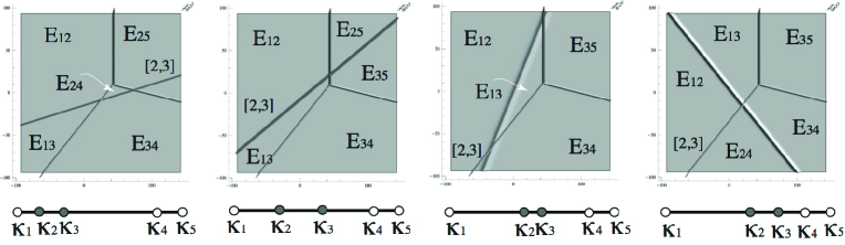
Figure 32. Examples of slides. These contour plots correspond to the same Le-diagram $L$ with $\pi(L)=(5,3,2,1,4)$, but these plots all differ from $G_{-}(L)$.

Lemma 11.6.

Consider the contour plot $\operatorname{\mathcal{C}}(u_{A},t)$ of a soliton solution coming from $A\in S_{L}^{tnn}$ at $t\ll 0$. Then its soliton graph either coincides with $G_{-}(L)$ or differs from it via a series of slides. Similarly, if one considers two contour plots of a soliton solution coming from $A\in S_{L}^{tnn}$ at $t\ll 0$, which are computed using different sets of parameters $(\kappa_{1},\dots,\kappa_{n})$, then one can be obtained from the other via a sequence of slides.

Proof. Theorem 8.5 gives a precise description of the trivalent vertices which appear in the contour plot, together with the topology of how they are connected to each other (including the circular order of the three line-solitons $[a,b]$, $[a,c]$, and $[b,c]$ incident to a given vertex $v_{a,b,c}$). In particular, the combinatorics of the trivalent vertices and their incident edges in the contour plot is precisely that which appears in $G_{-}(L)$.

The only feature of the contour plot which Theorem 8.5 does not determine is which pairs of line-solitons form an $X$-crossing. Therefore the topology of the contour plot may differ from that of $G_{-}(L)$ via a sequence of slides. In each slide, a line-soliton of type $[i,j]$ may pass across a trivalent vertex $v_{a,b,c}$, changing the location of the $X$-crossing, or possibly replacing one $X$-crossing with two $X$-crossings (or vice-versa). Note that the indices $\{i,j\}$ and $\{a,b,c\}$ must be disjoint, since an $X$-crossing involves two lines-solitons with disjoint indices.        

Lemma 11.7.

Consider two contour plots which differ by a single slide. Let $S_{1}$ and $S_{2}$ denote the two sets of Plücker coordinates corresponding to the dominant exponentials in the two contour plots. Then from the values of the Plücker coordinates in $S_{1}$, one can reconstruct the values of the Plücker coordinates in $S_{2}$, and vice-versa.

Proof. Recall from Theorem 9.1 that the four Plücker coordinates incident to an $X$-crossing are dependent, in particular they satisfy a “two-term” Plücker relation. Now it is easy to verify the lemma by inspection, since each slide only creates or removes one region, and there is a dependence among the Plücker coordinates labeling the dominant exponentials. The reader may wish to check this by looking at the first and second, or the second and third, or the third and fourth contour plots in Figure 32.        

We now turn to the proof of Theorem 11.4.

Proof. We consider the case that $t\ll 0$. By Lemma 11.1, we can identify the cell $S_{\pi}^{tnn}=S_{L}^{tnn}$ containing $A$. We can also compute the labels of the dominant exponentials in the contour plot and the values of the corresponding Plücker coordinates.

Define

$$\mathcal{T}=\left\{~{}I\in{[n]\choose k}~{}\Big{|}~{}E_{I}\text{ is a dominant exponential in }\operatorname{\mathcal{C}}(u_{A},t)~{}\right\}.$$

We now claim that from the values of each $\Delta_{I}(A)$ for $I\in\mathcal{T}$, we can determine $A$.

To prove the claim, note that since $t\ll 0$ sufficiently small, the contour plot $\operatorname{\mathcal{C}}(u_{A},t)$ has the same topology as $\operatorname{\mathcal{C}}_{-}(\mathcal{M})$. Therefore $\operatorname{\mathcal{C}}(u_{A},t)$ will either have the same topological structure as the graph $G_{-}(L)$, or by Lemma 11.6, it will differ from $G_{-}(L)$ via a sequence of slides. And so by Lemma 11.7, we can determine the values of the Plücker coordinates labeling the regions in $G_{-}(L)$.

We now use Theorem 11.14, below, which shows that from the values of the Plücker coordinates labeling the regions in $G_{-}(L)$, one can reconstruct all nonzero Plücker coordinates. This determines the point $A\in(Gr_{k,n})_{\geq 0}$.

This completes the proof of Theorem 11.4 for $t\ll 0$. The proof of the theorem for $t\gg 0$ just follows the same argument, with the dual $\Gamma$ -diagram (which is a relabeled $\Gamma$ -diagram) replacing the $\Gamma$ -diagram in the construction of the asymptotic contour plot.        

11.1. Reconstructing a point of $(Gr_{k,n})_{\geq 0}$ from a minimal set of Plücker coordinates

Talaska [31] studied the problem of how to reconstruct an element $A\in(Gr_{k,n})_{\geq 0}$ from a subset of its Plücker coordinates $\Delta_{I}(A)$. For each cell $S_{\mathcal{M}}^{tnn}$, she characterized a minimal set of Plücker coordinates which suffice to reconstruct the corresponding element of $S_{\mathcal{M}}^{tnn}$. Her proof worked by explicitly inverting Postnikov’s boundary measurement map [25]. In this section we review some of Talaska’s work.

Given a $\Gamma$ -diagram $L$ of shape $\lambda$ which fits inside a $k\times(n-k)$ rectangle, we construct a planar network $N_{L}$ as follows. First we draw a disk whose boundary consists of the north and west edges of the $k\times(n-k)$ box and the path determining the southeast boundary of $\lambda$. Place a vertex, called a boundary source, at the end of each row, and a vertex, called a boundary sink, at the end of each column of $\lambda$. Label these in sequence with the integers $\{1,2,\dots,n\}$, following the path from the northeast corner to the southwest corner which determines $\lambda$. Let $I=\{i_{1}<i_{2}<\dots<i_{k}\}$ be the set of boundary sources, so that $[n]\setminus I=\{j_{1}<j_{2}<\dots<j_{n-k}\}$ is the set of boundary sinks.

Given a box $b$ in $L$ which contains a $+$, we drop a hook down and to the right, extending the two segments comprising the hook all the way to the boundary of the disk. We direct the horizontal segment left and the vertical segment down. After forgetting the $+$’s and $0$’s in $L$, we now have a planar directed network. There is exactly one face for each box $b$ in $\lambda$ containing a $+$, and in addition, there is one face whose northwest boundary is the boundary of the disk. See the first two pictures in Figure 33, which shows this construction applied to the $\Gamma$ -diagram from Figure 10.

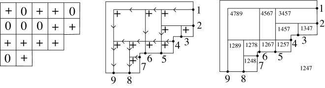
Figure 33. A minimal set of Plücker coordinates for $\pi=(7,4,2,9,1,3,8,6,5)$.

Talaska proved the following.

Theorem 11.8.

[31, Corollary 4.2], [31, Lemma 2.1] Let $L$ be the $\Gamma$ -diagram of a positroid cell $S_{L}^{tnn}$, and $A\in S_{L}^{tnn}$. Define a set of Plücker coordinates $T(L):=\{\Delta_{I}(A)\}\cup\{\Delta_{J(b)}(A)\}_{b}$, where $b$ ranges over all boxes containing a $+$ in the $\Gamma$ -diagram, and $J(b)$ is the destination set of the northwest-most path collection lying weakly southeast of the $b$ hook. Then $T(L)$ is a totally positive base; that is, each nonzero Plücker coordinate on $S_{L}^{tnn}$ can be written as a subtraction-free expression in the elements of $T(L)$. It follows that one can reconstruct $A$ from $T(L)$.

The right side of Figure 33 shows the Plücker coordinate $\Delta_{J(b)}$ associated with each box $b$ which contained a $+$ in the $\Gamma$ -diagram.

Definition 11.9.

Given a $\Gamma$ -diagram $L$ and a box $b$ containing a $+$, let $L_{b}$ be the $\Gamma$ -diagram obtained from $L$ by changing the content of each box to a $0$ if the box lies in a row above $b$ or a column left of $b$.

Definition 11.10.

We define a total order on elements of ${[n]\choose k}$ by saying that $J^{1}=\{j^{1}_{1}>\dots>j^{1}_{k}\}>J^{2}=\{j^{2}_{1}>\dots>j^{2}_{k}\}$ if in the first position $i$ where they differ, $j^{1}_{i}>j^{2}_{i}$. Then if $\mathcal{M}\subset{[n]\choose k}$, we refer to the largest element of $\mathcal{M}$ as lexicographically maximal.

The following lemma is implicit in [31].

Lemma 11.11.

Let $\mathcal{M}:=\mathcal{M}(L_{b})$ be the collection of Plücker coordinates which are positive on the cell $S_{L_{b}}^{tnn}$. Then $\Delta_{J(b)}$ is the lexicographically maximal element of $\mathcal{M}$.

The following lemma is obvious.

Lemma 11.12.

The generalized plabic graph $G_{-}(L_{b})$ that Algorithm 8.3 associates to $L_{b}$ is contained inside $G_{-}(L)$.

Lemma 11.13.

Consider the graph $G_{-}(L)$ constructed by Algorithm 8.3. Let $J$ be the $k$-element subset of $[n]$ which labels the region $R$ that comes from the northwest corner of the $\Gamma$ -diagram $L$ (see the bottom left picture in Figure 10). Then $J$ is the lexicographically maximal element of $\mathcal{M}(L)$.

Proof. One may prove directly that the label of $R$ coincides with the destination set of the northwest-most path collection in $N_{L}$.

Alternatively, we may prove this using a soliton argument. Let $A\in S_{L}^{tnn}$. When $x\gg 0$, we have that $E_{n}>E_{n-1}>\dots>E_{1}$. Therefore if $J$ is the lexicographically maximal element of $\mathcal{M}(L)$, then the term $\Delta_{J}(A)E_{J}$ dominates the $\tau$-function $\tau_{A}$. It follows that $E_{J}$ is the dominant exponential of any contour plot $\operatorname{\mathcal{C}}(u_{A},t)$ in the region where $x\gg 0$. By Lemma 11.6, for $t\ll 0$, this contour plot coincides with $G_{-}(L)$ up to a series of slides, none of which will change the label of the region at $x\gg 0$. And this region corresponds to the region coming from the northwest corner of the $\Gamma$ -diagram $L$.        

Theorem 11.14.

Let $L$ be a $\Gamma$ -diagram. Consider the set $S$ of Plücker coordinates associated to the dominant exponentials in the regions of the graph $G_{-}(L)$, as constructed in Algorithm 8.3. Then $S$ contains $T(L)$. In particular, one may reconstruct the element $A\in S_{L}^{tnn}$ from the values of the Plücker coordinates labeling $G_{-}(L)$ for $t\ll 0$.

Proof. By Lemmas 11.11, 11.12, and 11.13, for each box $b$ in $L$, $E_{J(b)}$ is a dominant exponential labeling a region of $G_{-}(L)$. Also, if $I$ is the lexicographically minimal element of $\mathcal{M}(L)$, then $E_{I}$ labels the region at $x\ll 0$ in $G_{-}(L)$. Therefore $T(L)\subset S$. The proof now follows from Theorem 11.8.        

12. Triangulations of $n$-gon and soliton graphs for $(Gr_{2,n})_{>0}$

The main result of this section is an algorithm for producing all generic soliton graphs (up to the (M2)-equivalence of Section 10.1) that come from $(Gr_{2,n})_{>0}$. We consider the generic asymptotic contour plot $\operatorname{\mathcal{C}}_{{\bf a}}(\mathcal{M})$ for each fixed ${\bf a}=(a_{3},\ldots,a_{m})$, and classify those plots by taking various choices of ${\bf a}$ in the $\mathbb{R}^{m-2}$-space. Here we will show that it is sufficient to consider $m=n-1$ for $n\geq 4$. Note that by Corollary 9.2, these asymptotic contour plots do not have any $X$-crossings, and hence their generic soliton graphs have only trivalent vertices. We state the algorithm and main theorem in Section 12.1, and then prove it in the rest of the section.

12.1. Algorithm to produce soliton graphs

Algorithm 12.1.

Let $T$ be a triangulation of an $n$-gon $P$, whose $n$ vertices are labeled by the numbers $1,2,\dots,n$, in counterclockwise order. Therefore each edge of $P$ and each diagonal of $T$ is specified by a pair of distinct integers between $1$ and $n$. The following procedure yields a labeled graph $\Psi(T)$.

1. Put a black vertex in the interior of each triangle in $T$.

2. Put a white vertex at each of the $n$ vertices of $P$ which is incident to a diagonal of $T$; put a black vertex at the remaining vertices of $P$.

3. Connect each vertex which is inside a triangle of $T$ to the three vertices of that triangle.

4. Erase the edges of $T$, and contract every pair of adjacent vertices which have the same color. This produces a new graph $G$ with $n$ boundary vertices, in bijection with the vertices of the original $n$-gon $P$.

5. Add one unbounded ray to each of the boundary vertices of $G$, so as to produce a new (planar) graph $\Psi(T)$. Note that $\Psi(T)$ divides the plane into regions; the bounded regions correspond to the diagonals of $T$, and the unbounded regions correspond to the edges of $P$. More specifically, a region of $\Psi(T)$ is labeled by $E_{ij}$, where $i$ and $j$ are the endpoints of the corresponding diagonal or edge of $T$.

See Figure 34. Our main result in this section is the following.

Theorem 12.2.

Up to (M2)-equivalence, the graphs $\Psi(T)$ constructed above are soliton graphs for $(Gr_{2,n})_{>0}$, and conversely, up to (M2)-equivalence, any generic soliton graph for $(Gr_{2,n})_{>0}$ comes from this construction. Moreover, one can realize each graph $\Psi(T)$ by choosing ${\bf a}=(a_{3},\dots,a_{n})$ appropriately.

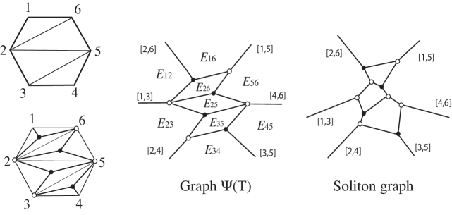
Figure 34. Algorithm 12.1, starting from a triangulation of a hexagon. The right figure shows the corresponding soliton graph from the contour plot for a soliton solution from $(Gr_{2,6})_{>0}$. The graph $\Psi(T)$ is (M2)-equivalent to the soliton graph.

Remark 12.3.

The process of flipping a diagonal in the triangulation corresponds to a mutation in the cluster algebra. In the terminology of reduced plabic graphs, a mutation corresponds to the square move (M1) (see Section 10.1). In the setting of KP solitons, each mutation may be considered as an evolution along a particular flow of the KP hierarchy. For example, the contour plot for $(Gr_{2,4})_{>0}$ for $t_{3}\ll 0$ has one bounded region with the dominant exponential $E_{1,3}$, and as $t_{3}$ increases, the bounded region closes at some $t_{3}$, then for $t_{3}\gg 0$, the contour plot has again one bounded region with the dominant exponential $E_{2,4}$. (This can be easily verified using the construction given in Section 8.) Thus, the time $t_{3}$ can be considered as a mutation parameter for $A_{1}$ cluster, i.e. $\Delta_{1,3}\to\Delta_{2,4}$ as $t_{3}$ increases.

Remark 12.4.

It is known already that the reduced plabic graphs for $(Gr_{2,n})_{>0}$ all have the form given by Algorithm 12.1 (up to (M2)-equivalence). And by Corollary 10.9, every generic soliton graph is a reduced plabic graph. Therefore it follows immediately that every generic soliton graph for $(Gr_{2,n})_{>0}$ must have the form of Algorithm 12.1. Therefore in order to prove Theorem 12.2, we must show that each graph that one can obtain from Algorithm 12.1 is realizable as a soliton graph (up to (M2)-equivalence).

12.2. Sequence of asymptotic contour plots

Let $\mathcal{M}={[n]\choose 2}$, the set of all two-element subsets of $[n]$. Recall that for fixed ${\bf a}=(a_{3},\ldots,a_{m})$ the asymptotic contour plot $\operatorname{\mathcal{C}}_{{\bf a}}(\mathcal{M})$ for $S_{\mathcal{M}}^{tnn}=(Gr_{2,n})_{>0}$ is defined as the locus in the $\bar{x}\bar{y}$-plane where

$$f_{\mathcal{M}}(\bar{x},\bar{y},{\bf a}):=\underset{1\leq i<j\leq n}{\text{max}}\left\{\Theta_{i,j}(\bar{x},\bar{y},{\bf a})\right\}$$

is not linear. Here $\Theta_{i,j}=\theta_{i}+\theta_{j}$ and

$$\theta_{j}(\bar{x},\bar{y},{\bf a})=\kappa_{j}\bar{x}+\kappa_{j}^{2}\bar{y}+\mathop{\textstyle\sum}\limits_{p=3}^{m}\kappa_{j}^{p}a_{p},\qquad\text{for}\quad j=1,\ldots,n.$$

Since $\mathcal{M}={[n]\choose 2}$ will be fixed throughout this section, we will hereafter refer to $\operatorname{\mathcal{C}}_{{\bf a}}(\mathcal{M})$ as simply $\operatorname{\mathcal{C}}_{{\bf a}}$.

For each fixed ${\bf a}$, we consider the $\binom{n}{2}$ planes defined by $z=\Theta_{i,j}(\bar{x},\bar{y},{\bf a})$ in the $(\bar{x},\bar{y},z)$-space. Then the asymptotic contour plot $\operatorname{\mathcal{C}}_{{\bf a}}$ represents the $\bar{x}\bar{y}$-projection of the intersection lines of those planes which take the largest values of $z$. We call those planes the dominant planes. Note that:

• If a point $(\bar{x},\bar{y})$ is not in $\operatorname{\mathcal{C}}_{{\bf a}}$ then there is a unique dominant plane at that point.

• Let $L_{i,j}$ be the line in the $\bar{x}\bar{y}$-plane where $\theta_{i}=\theta_{j}$. Every line segment of $\operatorname{\mathcal{C}}_{{\bf a}}$ (either bounded or unbounded) is a portion of some $L_{i,j}$.

• Given $\{i,j,k\}\subset[n]$, let $v_{i,j,k}=(v_{i,j,k}^{x},v_{i,j,k}^{y})$ be the point where the lines $L_{i,j}$, $L_{i,k}$, and $L_{j,k}$ mutually intersect. All trivalent vertices of $\operatorname{\mathcal{C}}_{{\bf a}}$ have the form $v_{i,j,k}$ for some $i,j,k$.

• If a point lies on a line of $\operatorname{\mathcal{C}}_{{\bf a}}$ then there are two dominant planes whose intersection gives the line, which breaks the linearity of $f_{\mathcal{M}}(\bar{x},\bar{y},{\bf a})$.

Lemma 12.5.

Let $(r_{1},\dots,r_{n})$ be any point in $\mathbb{R}^{n}$. Then we can find a unique point $(\bar{x},\bar{y},\mathbf{a})=(\bar{x},\bar{y},a_{3},\dots,a_{n-1})\in\mathbb{R}^{n-1}$ and a constant $a_{0}$ such that $\theta_{i}(\bar{x},\bar{y},{\bf a})=r_{i}-a_{0}$ for all $1\leq i\leq n$.

Proof. Define the function $\ell_{i}:\mathbb{R}\times\mathbb{R}^{n-1}\to\mathbb{R}$ by

$$\ell_{i}(a_{0},\bar{x},\bar{y},{\bf a})=a_{0}+\theta_{i}(\bar{x},\bar{y},{\bf a})=(a_{0},\bar{x},\bar{y},a_{3},\dots,a_{n-1})\cdot\mathsf{E}_{i}^{\bf 0},$$

where $\mathsf{E}_{i}^{\bf 0}$ is the $i$th column vector defined in (3.1). Recall that the matrix $E^{\bf 0}=(\mathsf{E}_{1}^{\bf 0},\ldots,\mathsf{E}_{n}^{\bf 0})$ is the Vandermonde matrix in the $\kappa_{j}$’s, and it is invertible. Therefore we can find a unique solution $(a_{0},\bar{x},\bar{y},{\bf a})$ to the equations $(a_{0},\bar{x},\bar{y},{\bf a})\cdot E^{\bf 0}=(r_{1},\ldots,r_{n})$, and hence $a_{0}+\theta_{i}(\bar{x},\bar{y},{\bf a})=r_{i}$ for all $i$.        

Lemma 12.5 implies that the relative positions of the planes $z=\Theta_{i,j}(\bar{x},\bar{y},{\bf a})$ at each point $(\bar{x},\bar{y})\in\mathbb{R}^{2}$ are determined by the $n-3$ parameters ${\bf a}=(a_{3},\ldots,a_{n-1})\in\mathbb{R}^{n-3}$.

In Theorem 12.7 below we will give a procedure for realizing each graph $\Psi(T)$ as a soliton graph (up to (M2)-equivalence). Note that by Remark 12.4, Theorem 12.2 is a consequence of Theorem 12.7.

First we need some definitions. Consider an $n$-gon, whose vertices are labeled from $1$ to $n$ in counterclockwise order, and let $I\subset[n]$. Choose some $j\in[n]\setminus I$. We say that the clockwise (respectively, counterclockwise) neighbor of $j$ in $I$ is the element of $I$ which is closest to $j$ when we travel from $j$ in clockwise (respectively, counterclockwise) order around the boundary of the polygon.

Definition 12.6.

Let $\mathcal{T}_{n}$ denote the triangulations of an $n$-gon, whose vertices are labeled from $1$ to $n$ in counterclockwise order. We define a surjective map $\lambda:S_{n}\to\mathcal{T}_{n}$ as follows. Let $(i_{1},\dots,i_{n})\in S_{n}$. We construct an element of $\mathcal{T}_{n}$ by:

• creating a triangle with vertices $\{i_{1},i_{2},i_{3}\}$

• For $4\leq k\leq n$, add two edges connecting $i_{k}$ to its clockwise and counterclockwise neighbors from $\{i_{1},i_{2},\dots,i_{k-1}\}$.

Theorem 12.7.

Choose a point $(r_{1},\dots,r_{n})\in\mathbb{R}^{n}$ such that

$$0=r_{i_{1}}=r_{i_{2}}=r_{i_{3}}\gg r_{i_{4}}\gg r_{i_{5}}\gg\cdots\gg r_{i_{n}}.$$

More specifically, choose some large real number $R$ such that

$$R \gg\underset{i\neq j\neq k}{\max}\left\{1,~{}\frac{1}{|\kappa_{k}-\kappa_{i}||\kappa_{k}-\kappa_{j}|},~{}\frac{|\kappa_{i}+\kappa_{j}|}{|\kappa_{k}-\kappa_{i}||\kappa_{k}-\kappa_{j}|}\right\}.$$

We then take

$$r_{i_{\ell}}=-R^{\ell}\qquad\text{for}\quad\ell=4,\ldots n.$$

Using Lemma 12.5, choose the unique point $(a_{0},\overline{x}_{0},\overline{y}_{0},a_{3},\dots,a_{n-1})$ such that $\theta_{i}(\overline{x}_{0},\overline{y}_{0},{\bf a})=r_{i}-a_{0}$ for all $1\leq i\leq n$. Then the soliton graph associated to the asymptotic contour plot $\operatorname{\mathcal{C}}_{{\bf a}}$ is (M2)-equivalent to the graph $\Psi(\lambda(i_{1},i_{2},\dots,i_{n}))$.

Remark 12.8.

Other choices of the $r_{i}$’s in Theorem 12.7 are possible, but the above choice will be convenient for our proofs.

From now on we use the hypotheses of Theorem 12.7.

Definition 12.9.

For $\ell=3,4,\dots,n$, we define

$$I_{\ell}:=\{i_{1},i_{2},\ldots,i_{\ell}\},$$

and

$$f^{(\ell)}(\bar{x},\bar{y},{\bf a}):=\underset{i,j\in I_{\ell}}{\text{max}}\left\{\Theta_{i,j}(\bar{x},\bar{y},{\bf a})\right\}.$$

And we define $\operatorname{\mathcal{C}}_{{\bf a}}^{(\ell)}$ to be the locus in the $\bar{x}\bar{y}$-plane where $f^{(\ell)}(\bar{x},\bar{y},{\bf a})$ is not linear.

We will prove Theorem 12.7 by induction on $n$. In order to justify the fact that we can build each contour plot inductively, we need the following result.

Proposition 12.10.

There is a sequence of regions $\mathcal{R}_{I_{\ell}}$

$$\mathcal{R}_{I_{3}}\subset\mathcal{R}_{I_{4}}\subset\cdots\subset\mathcal{R}_{I_{n}}=\mathbb{R}^{2}$$

in the $\bar{x}\bar{y}$-plane so that at any point $(\bar{x},\bar{y})\in\mathcal{R}_{I_{\ell}}$, we have the order

(12.1) $$\theta_{j}(\bar{x},\bar{y},{\bf a})~{}\gg~{}\theta_{i_{\ell+1}}(\bar{x},\bar{y},{\bf a})~{}\gg~{}\dots~{}\gg~{}\theta_{i_{n}}(\bar{x},\bar{y},{\bf a})$$

for any $j\in I_{\ell}$. Furthermore, every trivalent vertex $v_{i,j,k}$ of $\operatorname{\mathcal{C}}_{{\bf a}}$ is contained in the region $\mathcal{R}_{I_{k}}$.

Note that since $\theta_{i}(\bar{x}_{0},\bar{y}_{0},{\bf a})=r_{i}-a_{0}$, we have

$$\theta_{i}(\bar{x},\bar{y},{\bf a})=\kappa_{i}(\bar{x}-\bar{x}_{0})+\kappa_{i}^{2}(\bar{y}-\bar{y}_{0})+r_{i}-a_{0}.$$

Since each function $\theta_{i}$ is linear in $\bar{x}$ and $\bar{y}$, and because the asymptotic contour plots only depend on the orders of the values of the functions $\Theta_{i,j}$, we can assume without loss of generality that $\bar{x}_{0}=\bar{y}_{0}=a_{0}=0$. Or equivalently, we can always shift our coordinate system so that $(\bar{x}_{0},\bar{y}_{0},-a_{0})$ is the origin in the three-dimensional $\bar{x}\bar{y}z$-space. Therefore from now on we simply write

(12.2) $$z=\theta_{i}(\bar{x},\bar{y})=\theta_{i}(\bar{x},\bar{y},{\bf a})=\kappa_{i}\bar{x}+\kappa_{i}^{2}\bar{y}+r_{i}.$$

Using (12.2), the following lemma is easily verified.

Lemma 12.11.

The line $L_{i,j}$ in the $\bar{x}\bar{y}$-plane at which $\theta_{i}=\theta_{j}$ has the equation

$$\bar{x}+(\kappa_{i}+\kappa_{j})\bar{y}+\frac{r_{i}-r_{j}}{\kappa_{i}-\kappa_{j}}=0.$$

Given $\{i,j,k\}\subset[n]$, the vertex $v_{i,j,k}=(v_{i,j,k}^{x},v_{i,j,k}^{y})$ where the lines $L_{i,j}$, $L_{i,k}$, and $L_{j,k}$ mutually intersect has coordinates given by

$$v_{i,j,k}^{x} =\left(\frac{\kappa_{j}+\kappa_{k}}{(\kappa_{i}-\kappa_{j})(\kappa_{i}-\kappa_{k})}r_{i}+\frac{\kappa_{k}+\kappa_{i}}{(\kappa_{j}-\kappa_{i})(\kappa_{j}-\kappa_{k})}r_{j}+\frac{\kappa_{i}+\kappa_{j}}{(\kappa_{k}-\kappa_{i})(\kappa_{k}-\kappa_{j})}r_{k}\right)$$

$$v_{i,j,k}^{y} =-\left(\frac{r_{i}}{(\kappa_{i}-\kappa_{j})(\kappa_{i}-\kappa_{k})}+\frac{r_{j}}{(\kappa_{j}-\kappa_{i})(\kappa_{j}-\kappa_{k})}+\frac{r_{k}}{(\kappa_{k}-\kappa_{i})(\kappa_{k}-\kappa_{j})}\right).$$

We now prove Proposition 12.10.

Proof. By our choice of the constant $R$ and the $r_{i}$’s in Theorem 12.7, Lemma 12.11 implies that the distance $\|v_{i,j,k}\|$ from the point $v_{i,j,k}$ to the origin is approximately

$$\|v_{i,j,k}\|\approx\text{max}\{|r_{i}|,|r_{j}|,|r_{k}|\}.$$

Then for $3\leq\ell\leq n-1$, we let $\mathcal{R}_{I_{\ell}}$ denote the circle around the origin with radius equal to $R^{\ell+\frac{1}{2}}.$ (We let $\mathcal{R}_{I_{n}}=\mathbb{R}^{2}$.) Then it follows that each vertex $v_{i,j,k}$ for $i,j,k\in I_{\ell}$ lies in $\mathcal{R}_{I_{\ell}}$, and all others are outside this region. It is also immediate that in $\mathcal{R}_{I_{\ell}}$, (12.1) holds for any $j\in I_{\ell}$.        

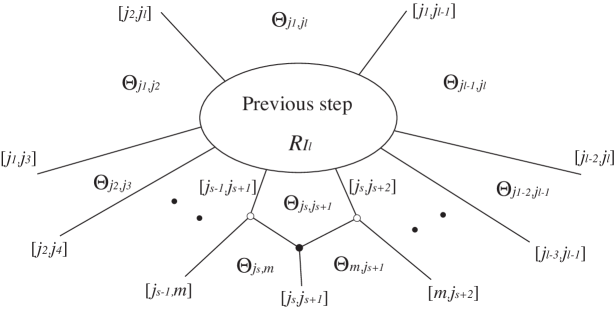
Figure 35. The unbounded region labeled by $\Theta_{j_{s},j_{s}+1}$ in $\operatorname{\mathcal{C}}_{{\bf a}}^{(\ell)}$ becomes bounded in $\operatorname{\mathcal{C}}_{{\bf a}}^{(\ell+1)}$. Here we have $j_{1}<\dots<j_{s}<m<j_{s+1}<\dots<j_{\ell}$ with $I_{\ell}=\{i_{1},\ldots,i_{\ell}\}$ and $I_{\ell+1}=I_{\ell}\cup\{m\}$.

We’re now ready to prove Theorem 12.7.

Proof. Note that $\operatorname{\mathcal{C}}_{{\bf a}}^{(\ell)}$ is an asymptotic contour plot for $(Gr_{2,\ell})_{>0}$, where the indices of the line-solitons come from the set $I_{\ell}$. By Proposition 12.10, we see the “whole” contour plot for $\operatorname{\mathcal{C}}_{{\bf a}}^{(\ell)}$ within the region $\mathcal{R}_{I_{\ell}}$, i.e. we see every trivalent vertex and a portion of every unbounded line-soliton. Moreover, (12.1) guarantees that if $\Theta_{i,j}$ is a dominant plane in some region of $\operatorname{\mathcal{C}}_{{\bf a}}^{(\ell)}$, then it remains a dominant plane in some region of $\operatorname{\mathcal{C}}_{{\bf a}}^{(\ell+1)}$.

Write $I_{\ell}=\{j_{1},j_{2},\dots,j_{\ell}\}$, where $j_{1}<j_{2}<\dots<j_{\ell}$, and write $m=i_{\ell+1}$. Since $\operatorname{\mathcal{C}}_{{\bf a}}^{(\ell+1)}$ is an asymptotic contour plot for $(Gr_{2,\ell+1})_{>0}$ with labels on the line-solitons and regions coming from the set $I_{\ell+1}$, the dominant planes labeling the unbounded regions of $\operatorname{\mathcal{C}}_{{\bf a}}^{(\ell+1)}$ correspond to all cyclically adjacent pairs in the set $I_{\ell}\cup\{m\}$. For example, if $j_{s}<m<j_{s+1}$, then those dominant planes are $\{\Theta_{j_{1},j_{2}},\Theta_{j_{2},j_{3}},\dots,\Theta_{j_{s},m},\Theta_{m,j_{s+1}},\dots,\Theta_{j_{\ell-1},j_{\ell}},\Theta_{j_{1},j_{\ell}}\}$. Among these, $\operatorname{\mathcal{C}}_{{\bf a}}^{(\ell+1)}$ contains two new dominant planes that $\operatorname{\mathcal{C}}_{{\bf a}}^{(\ell)}$ did not, namely $\Theta_{j_{s},m}$ and $\Theta_{m,j_{s+1}}$ – see Figure 35.

Now we know that:

• the soliton graph for $\operatorname{\mathcal{C}}_{{\bf a}}^{(\ell+1)}$ has the form $\Psi(T)$ for some triangulation $T$ of a polygon with vertices $I_{\ell+1}$.

• If $T^{\prime}=\lambda(i_{1},\dots,i_{\ell})$, then since $\operatorname{\mathcal{C}}_{{\bf a}}^{(\ell)}=\Psi(T^{\prime})$ up to (M2)-equivalence (by induction), and each dominant plane of $\operatorname{\mathcal{C}}_{{\bf a}}^{(\ell)}$ remains a dominant plane of $\operatorname{\mathcal{C}}_{{\bf a}}^{(\ell+1)}$, it follows that $T$ contains all the edges and diagonals that $T^{\prime}$ does.

• $\operatorname{\mathcal{C}}_{{\bf a}}^{(\ell+1)}$ contains $\Theta_{j^{-},m}$ and $\Theta_{m,j^{+}}$ as dominant planes, where $j^{-}$ and $j^{+}$ are the clockwise and counterclockwise neighbors of $m$ in the set $I_{\ell}$, and hence $T$ contains two edges or diagonals labeled by $(j^{-},m)$ and $(m,j^{+})$. (In Figure 35, where we have $j_{s}<m<j_{s+1}$, we have $\{j^{+},j^{-}\}=\{j_{s},j_{s+1}\}$.)

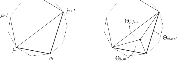
Figure 36. Adding a new vertex $m$ to the triangulation together with one new triangle with the vertices $\{j_{s},m,j_{s+1}\}$; and the effect on the graph $\Psi(T)$ produced from Algorithm 12.1. The regions are labeled by the dominant planes $\Theta_{i,j}$.

The only $T$ with all the properties above is the triangulation obtained from $T^{\prime}$ by inserting a new vertex $m=i_{\ell+1}$ in between its clockwise and counterclockwise neighbors $j^{-}$ and $j^{+}$, and connecting it by edges to those two vertices, see Figure 36. This completes the proof.

References

- [1] M. J. Ablowitz and P. A. Clarkson, Solitons, nonlinear evolution equations and inverse scattering (Cambridge University Press, Cambridge, 1991).
- [2] G. Biondini and S. Chakravarty, Soliton solutions of the Kadomtsev-Petviashvili II equation, J. Math. Phys., 47 (2006) 033514 (26pp).
- [3] G. Biondini, Y. Kodama, On a family of solutions of the Kadomtsev-Petviashvili equation which also satisfy the Toda lattice hierarchy, J. Phys. A: Math. Gen. 36 (2003), 10519–10536.
- [4] S. Chakravarty, Y. Kodama, Classification of the line-solitons of KPII, J. Phys. A: Math. Theor. 41 (2008) 275209 (33pp).
- [5] S. Chakravarty, Y. Kodama, A generating function for the N-soliton solutions of the Kadomtsev-Petviashvili II equation, Contemp. Math., 471 (2008), 47–67.
- [6] S. Chakravarty, Y. Kodama, Soliton solutions of the KP equation and applications to shallow water waves, Stud. Appl. Math. 123 (2009) 83–151.
- [7] L. A. Dickey, Soliton equations and Hamiltonian systems, Advanced Series in Mathematical Physics, Vol. 12, (World Scientific, Singapore, 1991).
- [8] A. Dimakis, F. Müller-Hoissen, KP line-solitons and Tamari lattices, J. Phys. A: Math. Theor. 44 (2011), 025203 (49pp).
- [9] S. Fomin, A. Zelevinsky, Cluster Algebras I: Foundations, J. Amer. Math. Soc. 15 (2002), 497-529.
- [10] N. Freeman, J. Nimmo, Soliton-solutions of the Korteweg-deVries and Kadomtsev-Petviashvili equations: the Wronskian technique, Phys. Lett. A 95 (1983), 1–3.
- [11] M. Gross, Tropical geometry and mirror symmetry, book available at http://www.math.ucsd.edu/~mgross/kansas.pdf.
- [12] R Hirota, The Direct Method in Soliton Theory (Cambridge University Press, Cambridge, 2004).
- [13] B. B. Kadomtsev and V. I. Petviashvili, On the stability of solitary waves in weakly dispersive media, Sov. Phys. - Dokl. 15 (1970) 539-541.
- [14] A. Knutson, T. Lam, and D. Speyer, Positroid varieties: juggling and geometry, to appear in Compositio.
- [15] Y. Kodama, Young diagrams and -soliton solutions of the KP equation, J. Phys. A: Math. Gen., 37 (2004) 11169-11190.
- [16] Y. Kodama, KP solitons in shallow water, J. Phys. A: Math. Theor. 43 (2010) 434004 (54pp).
- [17] Y. Kodama, L. Williams, KP solitons, total positivity, and cluster algebras, Proc. Natl. Acad. Sci., published online ahead of print May 11, 2011, doi:10.1073/pnas.1102627108.
- [18] Y. Kodama, L. Williams, The Deodhar decomposition of the Grassmannian and the regularity of KP solitons, Advances in Mathematics 244 (2013), 979–1032.
- [19] G. Lusztig, Total positivity in partial flag manifolds, Representation Theory, 2 (1998) 70-78.
- [20] G. Lusztig, Total positivity in reductive groups, in: Lie theory and geometry: in honor of Bertram Kostant, Progress in Mathematics 123, Birkhauser, 1994.
- [21] D. Maclagan, B. Sturmfels, Introduction to Tropical Geometry, in preparation.
- [22] T. Miwa and M. Jimbo and E. Date, Solitons: differential equations, symmetries and infinite-dimensional algebras (Cambridge University Press, Cambridge, 2000).
- [23] S. Novikov, S. V. Manakov, L. P. Pitaevskii and V. E. Zakharov, Theory of Solitons: The Inverse Scattering Method, Contemporary Soviet Mathematics, (Consultants Bureau, New York and London, 1984).
- [24] S. Oh, A. Postnikov, D. Speyer, Weak separation and plabic graphs, http://front.math.ucdavis.edu/arXiv:1109.4434.
- [25] A. Postnikov, Total positivity, Grassmannians, and networks, http://front.math.ucdavis.edu/math.CO/0609764.
- [26] A. Postnikov, D. Speyer, L. Williams, Matching polytopes, toric geometry, and the non-negative part of the Grassmannian, J. Alg. Combin., 30, 2009, 173–191.
- [27] M. Sato, Soliton equations as dynamical systems on an infinite dimensional Grassmannian manifold, RIMS Kokyuroku (Kyoto University) 439 (1981), 30–46.
- [28] J. Satsuma, A Wronskian representation of -soliton solutions of nonlinear evolution equations, J. Phys. Soc. Japan, 46 (1979) 356-360.
- [29] J. Scott, Grassmannians and cluster algebras, Proc. London Math. Soc. (3) 92 (2006), 345–380.
- [30] E. Steingrimsson, L. Williams, Permutation tableaux and permutation patterns, J. Comb. Th. A, 114, 2007, 211–234.
- [31] K. Talaska, Combinatorial formulas for -coordinates in a totally nonnegative Grassmannian, J. Combin. Theory Ser. A 118 (2011), no. 1, 58–66.
- [32] G. B. Whitham, Linear and nonlinear waves. Pure and Applied Mathematics. Wiley-Interscience (John Wiley and Sons), New York - London - Sydney, 1974. xvi+636 pp.