Topological Entanglement Entropy of $Z_{2}$ Spin liquids and Lattice Laughlin states

Abstract

We study entanglement properties of candidate wave-functions for $SU(2)$ symmetric gapped spin liquids and Laughlin states. These wave-functions are obtained by the Gutzwiller projection technique. Using Topological Entanglement Entropy $\gamma$ as a tool, we establish topological order in chiral spin liquid and $Z_{2}$ spin liquid wave-functions, as well as a lattice version of the Laughlin state. Our results agree very well with the field theoretic result $\gamma=\log D$ where $D$ is the total quantum dimension of the phase. All calculations are done using a Monte Carlo technique on a $12\times 12$ lattice enabling us to extract $\gamma$ with small finite size effects. For a chiral spin liquid wave-function, the calculated value is within $4\%$ of the ideal value. We also find good agreement for a lattice version of the Laughlin $\nu=1/3$ phase with the expected $\gamma=\log\sqrt{3}$.

I Introduction

Quantum Spin Liquids(SLs) are states that arise from the collective behavior of spins, but are not characterized by a Landau order parameter. They are associated with remarkable phenomena such as fractional quantum numbers anderson1987 , transmutation of statistics (eg. fermions appearing in a purely bosonic model)kivelson1987 ; read1989 , and enabling otherwise impossible quantum phase transitionssenthil2004 , to name a few. SLs may be gapless or gapped. While current experimental candidates for SLs appear to have gapless excitations exp , gapped SLs are indicated in numerical studies on the Kagome yan2010 and honeycomb lattice meng2010 . Gapped SLs are characterized by topological order - i.e. ground state degeneracy that depends on the topology of the underlying spacewen2004 .

Recently, a novel characterization of gapped SLs has emerged using quantum entanglement in terms of the Topological Entanglement Entropy (TEE)hamma2005 ; levin2006 ; kitaev2006 . This quantity takes a fixed value $\gamma$ in a topologically ordered phase and remarkably can be calculated just knowing the ground state wave-function. The entanglement entropy of a two dimensional disc shaped region A in a gapped phase obeys $S_{2}=al_{A}-\gamma$, where a smooth boundary of length $l_{A}$ is assumed to surround the region. By carefully subtracting off the leading dependence, the constant $\gamma$ can be isolated. It is argued to be a characteristic of the phase, $\gamma=\log D$, where $D$ is the quantum dimension of the phase levin2006 ; kitaev2006 . For the abelian states discussed here, $D^{2}$ is identical to the ground state degeneracy on the torus.

Gapped SLs can be viewed as a state where each spin forms a singlet with a near neighbor, but the arrangement of singlets fluctuates quantum mechanically so it is a liquid of singlets. Theoretical models of this singlet liquid fall roughly into two categories. In the first, the singlets are represented as microscopic variables as in quantum dimer and related modelsrokhsar1988 ; moessner2001 ; senthil2002 ; balents2002 ; misguich , and are suggested by large N calculations sachdev1992 . Topological order can then be established by a variety of techniques including exact solution and most recently quantum entanglement Furukawa ; Claudio ; Fradkin ; isakov2011 ; hamma2008 . In contrast there has been less progress establishing topological order in the second category, which are SU(2) symmetric spin systems where valence bonds are emergent degrees of freedom. Andersonanderson1987 proposed constructing an SU(2) symmetric SL wave-function by starting with a BCS state, derived from the mean field Hamiltonian:

$$H=-\sum_{rr^{\prime}}\{t_{rr^{\prime}}f^{\dagger}_{\sigma,r}f_{\sigma,r^{\prime}}+\Delta_{rr^{\prime}}f^{\dagger}_{\uparrow,r}f^{\dagger}_{\downarrow,r^{\prime}}\}+h.c.$$ (1)

and Gutzwiller projecting it so that there is exactly one fermion per site, hence a spin wave-function. Variants of these are known to be good variational ground states for local spin Hamiltonians (see e.g. varstudy ) and are more viable descriptions of most experimental and $SU(2)$ symmetric liquids. Approximate analytical treatments of projection, that include small fluctuations about the above mean field state, indicate that at least two kinds of gapped SLs can arise: chiral SLskalmeyer and $Z_{2}$ SLs sachdev1992 ; wen1991 ; senthil2000 . However, given the drastic nature of projection, it is unclear if the actual wave-functions obtained from this procedure are in the same phases. In this paper we use TEE to establish topological order for of $SU(2)$ symmetric chiral and $Z_{2}$ SL wave-functions. We show that the recently developed Monte Carlo technique used to study entanglement properties of gapless SLsfrank2011 can be applied here as well to extract TEE for system sizes large enough (144 spins) so that it approaches its quantized value. Instead of using the more standard Von Neumann entropy, we focus on the Renyi entropy, which carries the same contribution from the TEE for both non-chiral flammia2009 and chiral dong states for a topologically trivial bipartition. The fact that the wave-function is a determinant or product of determinants in these cases allows for its efficient evaluation. For a model of of the chiral SL, the calculated TEE are remarkably accurate, within few percent of the expected $\log\sqrt{2}$ value. To our knowledge, this is the first clear demonstration of topological order via TEE, in SU(2) symmetric spin wave-functions.

We also study lattice versions of the Laughlin $\nu=1/3$ state, which are obtained by a similar projective construction, although these are fermionic, not spin wave-functions. Again we can extract TEE which is within 7% of the expected value to confirm these are in the same phase as the Laughlin state, although they differ significantly in microscopic structure.

We note earlier numerical work extracting TEE include exact digitalization studies on small systems, looking at quantum Hall Laughlin states haque2007 and perturbed Kitaev toric code modelshamma2008 . Recently, a quantum Monte Carlo study isakov2011 used TEE to detect $Z_{2}$ topological order. In contrast to the states studied here, this was a positive definite wave-function, with U(1) rather than SU(2) spin symmetry. Our wave-function-only approach is ready-made for searching for topological order when one has a good variational ansatz for a ground state, irrespective of whether the state is positive definite or not. Finally, we note that Ref. ivanov2002 studied topological order in ‘nodal’ $Z_{2}$ SLs by constructing four orthogonal low energy states on the torus, and Ref. Yao studied TEE for the Kitaev model.

The format of the paper and main results are summarized in the section below.

In Section II the TEE $\gamma$ is defined, and an algorithm to calculate it numerically utilizing the Renyi entanglement entropy $S_{2}$ is outlined. This is then applied to a series of topological phases, the results of which are summarized in table 1.

(i) The first is a Chern insulator, built out of a square lattice tight binding model at half filling, in which the filled band has unit Chern number. For a lattice with $2N$ sites, this is an N body Slater determinant $\Phi(r_{1},\dots,\,r_{N})$. Since this is an integer quantum Hall state, it is not expected to possess topological order. Indeed, calculation is consistent with a vanishing TEE, see Table 1 first row.

(ii) The chiral SL wave-function is obtained from the wave-function of 2N spinful electrons with this tight binding band structure, by projecting out all double occupancies, and studied in Section III. The chiral SL wave-function can be written as a product of two Slater determinants, i.e.$\Psi(r_{1},\,r_{2}\dots,\,r_{N})={\mathcal{M}}\Phi^{2}(r_{1},\dots,\,r_{N})$, where ${\mathcal{M}}$ an unimportant Marshall sign factor. If we view up spin as a hardcore boson, then this is the wave-function analogous to half filled Landau level $\nu=1/2$ of bosons. It is therefore expected to have $\gamma=\log\sqrt{2}$. Indeed, for a particular choice of parameters with a large gap, numerical calculation (second and third rows of table 1, with different linear dimensions $L_{A}$ of the smallest subregions involved) yields a value very close to this. Detailed finite size analysis obtained by varying the correlation length of the chiral SL is presented in Section III, providing further evidence for convergence to the expected value. We note that this wave-function is SU(2) symmetric, and non-positive-definite, since the ground state is not time reversal symmetric.

(iii) Note, the construction of the chiral SL above is similar to the Laughlin construction of fractional quantum Hall states by taking products of the integer quantum Hall states. Extending the construction above, one can write wave-functions for $N$ fermions $\Psi_{1/3}(r_{1},\,r_{2}\dots,\,r_{N})=\Phi^{3}(r_{1},\dots,\,r_{N})$, a lattice version of the Laughlin $\nu=1/3$ state. The entanglement entropy calculation for $\Psi_{1/3}$ agrees well with what is expected for the topological order for $\nu=1/3$ Laughlin state, indicating it is in the same phase, despite not being constructed from lowest Landau level states. Note, since they differ significantly in microscopic detail from the Laughlin state, wave-function overlap is not an option in establishing that they are in the same phase. Also, calculating entanglement spectra li2008 is currently not feasible for these wave-functions, thus TEE appears to be the ideal characterization. Similarly, the lattice analog of Laughlin $\nu=1/4$ state for bosons, obtained via $\Psi_{1/4}(r_{1},\,r_{2}\dots,\,r_{N})=\Phi^{4}(r_{1},\dots,\,r_{N})$, is found to have a TEE close to the expected $\gamma=\log\sqrt{4}$, as discussed in Section IV.

(iv) Finally, we construct a fully gapped $Z_{2}$ SL wave-function on the square lattice. For the largest system sizes we considered, the calculated $\gamma$ is $84\%$ of the expected $\log 2$ value(last row in table 1). The difference is ascribed to larger finite size effects, as discussed in Section V.

State	Expected $\gamma$	$\gamma_{\rm calculated}/\gamma_{\rm expected}$
Unprojected ($\nu=1$)	0	-0.0008$\pm$ 0.0059 ∗
Chiral SL LA=3	$\log\sqrt{2}$	0.99 $\pm$ 0.03
Chiral SL LA=4	$\log\sqrt{2}$	0.99 $\pm$ 0.12
Lattice $\nu=1/3$	$\log\sqrt{3}$	1.07$\pm$ 0.05
Lattice $\nu=1/4$	$\log\sqrt{4}$	1.06 $\pm$ 0.11
Z2 SL LA=4	$\log{2}$	0.84 $\pm$ 0.13

Table 1: Comparison between calculated TEE and expected value from field theory(second column) for topological phases. The ^∗ denotes that the calculated value is not divided by the expected value since the latter vanishes.

II Topological entanglement entropy and Variational Monte Carlo method

II.1 Renyi entropy and topological entanglement entropy

Given a normalized wave-function $\left|\Phi\right\rangle$ and a partition of the system into subsystems $A$ and $B$, one can trace out the subsystem $B$ to obtain the reduced density matrix on $A$: $\rho_{A}=Tr_{B}\left|\Phi\right\rangle\left\langle\Phi\right|$. The Renyi entropies are defined as:

$$S_{n}=\frac{1}{1-n}\log\left(Tr\rho^{n}_{A}\right)$$ (2)

Taking the limit $n\rightarrow 1$, this recovers the definition of the usual von Neumann entropy. In this paper we will focus on the Renyi entropy with index $n=2$: $S_{2}=-\log\left(Tr\left(\rho^{2}_{A}\right)\right)$, which is easier to calculate with our Variational Monte Carlo(VMC) method frank2011 .

For a gapped phase in 2D with topological order, a contractible region $A$ with smooth boundary of length $l_{A}$, the Area Law of the Renyi entropy becomes:

$$S_{2}=al_{A}-\gamma$$

where we have omitted the sub-leading terms. Although the coefficient $a$ of the leading boundary law’ term is non-universal, the sub-leading constant $\gamma$ is universal, and this TEE is a robust property of the phase of matter for which $|\Phi\rangle$ is the ground state. It is given by $\gamma=\log D$, where $D$ is the total quantum dimension of the model levin2006 ; kitaev2006 , and offers a partial characterization of the underlying topological order. When region $A$ has a disc geometry, it has been shown that $\gamma$ for different Renyi indices $n$ are identical for both chiral and non-chiral statesflammia2009 ; dong . A simple limit where this is readily observedhamma2005 ; levin2006 is in a model wave-function of a $Z_{2}$ SL, which is an equal superposition of loops ($Z_{2}$ electric field). This is achieved as a ground state in Kitaev’s toric code model kitaev2003 . The Schmidt decomposition into wave-functions in regions $A$ and $B$ can be indexed by the configuration of electric field lines piercing the boundary of the disc. If $i=1,2,\dots l$ are $l$ bonds going through the boundary between region $A$ and $B$, the presence (absence) of electric field lines on bond $i$ is denoted by $q_{i}=1$ ($q_{i}=0$). Since the loops are closed, we require $\sum_{i}q_{i}={\rm even}$. It can be shown that the wave-function is simply an equal weight decomposition indexed by all possible configurations of $q_{i}$. There are $C=2^{l-1}$ of them, the global constraint of closed loops accounting for the missing factor of $2$. Then:

$$|\Psi\rangle=\frac{1}{\sqrt{C}}\sum_{q_{1}+\dots+q_{l}\,{\rm even}}|\Psi^{A}_{q_{1}\dots q_{l}}\rangle|\Psi^{B}_{q_{1}\dots q_{l}}\rangle$$

This implieslevin2006 there are $C$ equal eigenvalues of the region A density matrix, each equal to $1/C$. The Renyi entropy from Eqn.2 is: $S_{n}=\frac{1}{1-n}\log C^{-(n-1)}=(l-1)\log 2$. Thus $\gamma=\log 2$ from the definition above, if we identify $l$ with the length of the boundary. Note, this follows independent of the Renyi index $n$, and is the expected value for a $Z_{2}$ gauge theory with quantum dimension $D=2$.

Practically, it is not convenient to extract the subleading constant by fitting the expression above, particularly on the lattice where edges frequently occur. Instead, one may use a construction due to Levin and Wenlevin2006 , or Kitaev and Preskillkitaev2006 , that effectively cancels out the leading term and exposes the topological contribution. We use the latter, which requires calculating entanglement entropy for a triad of non overlapping regions A, B, C, and their various unions, and then constructing:

$$-\gamma = S_{A}+S_{B}+S_{C}-S_{AB}-S_{AC}-S_{BC}+S_{ABC}$$

here, any $S_{n}$ can be used, and we choose to use $S_{2}$, since it can be easily calculated. This guarantees that the contributions of boundaries and corners cancel when the dimensions of individual regions $A,B,C$ is much larger than the correlation length.

II.2 Variational Monte Carlo method for Renyi Entropy

In this section we briefly review the VMC algorithm for calculating Renyi entropy $S_{2}$ hastings2010 ; frank2011 . Consider the configurations $|\alpha_{1}\rangle=|a\rangle|b\rangle$, $|\alpha_{2}\rangle=|a^{\prime}\rangle|b^{\prime}\rangle$, $|\beta_{1}\rangle=|a^{\prime}\rangle|b\rangle$, $|\beta_{2}\rangle=|a\rangle|b^{\prime}\rangle$, where $|a\rangle$ and $|a^{\prime}\rangle$ have their support only in the subsystem $A$ while $|b\rangle$ and $|b^{\prime}\rangle$ are in subsystem $B$. Following Ref.hastings2010 , we define an operator $\rm{Swap_{A}}$ that acts on the tensor product of two copies of the system and swaps the configurations of the spins belonging to the $A$ subsystem in the two copies i.e. $\rm{Swap_{A}}|\alpha_{1}\rangle\otimes|\alpha_{2}\rangle=|\beta_{1}\rangle\otimes|\beta_{2}\rangle$. The Renyi entropy $S_{2}$ for the bipartition $A$ and $B$ can be expressed in terms of the expectation value of $\rm{Swap_{A}}$ with respect to the wave-function $|\Phi\rangle\otimes|\Phi\rangle$:

$$S_{A}=-\log\left(tr\rho_{A}^{2}\right)=-\log\left<\rm{Swap_{A}}\right>$$ (3)

$<\rm{Swap_{A}}>$ may be re-expressed as a Monte Carlo average:

$$\left<\rm{Swap_{A}}\right>=\underset{\alpha_{1},\alpha_{2}}{\sum}\rho_{\alpha_{1}}\rho_{\alpha_{2}}f\left(\alpha_{1},\alpha_{2}\right)$$ (4)

where the weights $\rho_{\alpha_{i}}=\left|\left\langle\alpha_{i}|\Phi\right\rangle\right|^{2}/\sum_{\alpha_{i}}\left|\left\langle\alpha_{i}|\Phi\right\rangle\right|^{2}$ are normalized and non-negative while the quantity to be averaged over the probability distribution $\rho_{\alpha_{1}}\rho_{\alpha_{2}}$ is:

$$f\left(\alpha_{1},\alpha_{2}\right)=\frac{\left\langle\beta_{1}|\Phi\right\rangle\left\langle\beta_{2}|\Phi\right\rangle}{\left\langle\alpha_{1}|\Phi\right\rangle\left\langle\alpha_{2}|\Phi\right\rangle}$$ (5)

Therefore, one can calculate the Renyi entropy using VMC method. This technique is particularly suited for projected wave-functions since the projection is rather easy to implement in a VMC algorithm gros1989 . As shown in Ref. frank2011 VMC algorithm correctly reproduces the exact results for free fermions with an error of less than a few percent.

We further facilitate our calculation with an algorithm that we referred to as the sign trickfrank2011 . It offers simplification and reduces computational cost. Basically, we separate $\left<\rm{Swap_{A}}\right>$ as a product of two factors, which may be independently calculated within VMC method:

$$\left\langle\rm{Swap_{A}}\right\rangle = \langle\rm{Swap_{A,mod}}\rangle\langle\rm{Swap_{A,sign}}\rangle$$

$$= \underset{\alpha_{1}\alpha_{2}}{\sum}\rho_{\alpha_{1}}\rho_{\alpha_{2}}|f\left(\alpha_{1},\alpha_{2}\right)|\left[\underset{\alpha_{1}\alpha_{2}}{\sum}\tilde{\rho}_{\alpha_{1},\alpha_{2}}e^{i\phi\left(\alpha_{1},\alpha_{2}\right)}\right]$$

The first factor is the Renyi entropy of a sign problem free wave-function $|\phi_{\alpha_{i}}|$. The second term is the expectation value of the phase factor $e^{i\phi\left(\alpha_{1},\alpha_{2}\right)}=\phi^{*}_{\alpha_{1}}\phi^{*}_{\alpha_{2}}\phi_{\beta_{1}}\phi_{\beta_{2}}/\left|\phi^{*}_{\alpha_{1}}\phi^{*}_{\alpha_{2}}\phi_{\beta_{1}}\phi_{\beta_{2}}\right|$ with probability distribution $\tilde{\rho}_{\alpha_{1},\alpha_{2}}=|\phi^{*}_{\alpha_{1}}\phi^{*}_{\alpha_{2}}\phi_{\beta_{1}}\phi_{\beta_{2}}|/\underset{\alpha_{1}\alpha_{2}}{\sum}|\phi^{*}_{\alpha_{1}}\phi^{*}_{\alpha_{2}}\phi_{\beta_{1}}\phi_{\beta_{2}}|$. Both factors can be calculated in a more efficient manner and most importantly, have much smaller errors than the direct calculation of $\left\langle\rm{Swap_{A}}\right\rangle$.

III Entanglement entropy for a chiral spin liquid

In this section we calculate the Renyi entropy $S_{2}$ and TEE $\gamma$ for a chiral SLkalmeyer .

III.1 Projected wave-function for chiral spin liquids

The chiral SL is a spin SU(2) singlet ground state, that breaks time reversal and parity symmetrykalmeyer ; thomale . A wave-function in this phase wave function may be obtained using the slave-particle formalism by Gutzwiller projecting a $d+id$ BCS state kalmeyer . Alternately, it can be obtained by Gutzwiller projection of a hopping model on the square lattice. This model has fermions hopping on the square lattice with a $\pi$ flux through every plaquette and imaginary hoppings across the square lattice diagonals:

$$H=\underset{\left\langle ij\right\rangle}{\sum}t_{ij}f_{i}^{\dagger}f_{j}+i\underset{\left\langle\left\langle ik\right\rangle\right\rangle}{\sum}\Delta_{ik}f_{i}^{\dagger}f_{k}$$ (6)

Here $i$ and $j$ are nearest neighbors and the hopping amplitude $t_{ij}$ is $t$ along the $\hat{y}$ direction and alternating between $t$ and $-t$ in the $\hat{x}$ direction from row to row; and $i$ and $k$ are second nearest neighbors connected by hoppings along the square lattice diagonals, with amplitude $\Delta_{ik}=i\Delta$ along the arrows and $\Delta_{ik}=-i\Delta$ against the arrows, see Fig. 1. The unit cell contains two sublattices $A$ and $B$. This model leads to a gapped state at half filling and the resulting valence band has unit Chern number. This hopping model is equivalent to a $d+id$ BCS state by an $SU\left(2\right)$ Gauge transformationludwig1994 . We use periodic boundary conditions throughout this section.

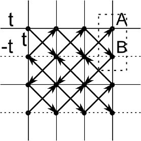
Figure 1: Illustration of a square lattice hopping model connected with a $d+id$ superconductor. While the nearest neighbor hopping is along the square edges with amplitude $t$ ($-t$ for hopping along dashed lines), the second nearest neighbor hopping is along the square diagonal (arrows in bold), with amplitude $+i\Delta$ ($-i\Delta$) when hopping direction is along (against) the arrow. The two sublattices in the unit cell are marked as $A$ and $B$.

The unprojected ground state wave-function $|\phi\rangle$ is obtained by filling all the states in the valence band ($\epsilon_{k}<0$) i.e. $|\phi\rangle=\left[\underset{k,s}{\Pi}\gamma^{\dagger}_{sk}\right]|0\rangle$ where $\gamma^{\dagger}_{k,s}=\psi_{A}(k)\underset{r_{A}}{\sum}f^{\dagger}_{r_{A},s}e^{ik\cdot r_{A}}+\psi_{B}(k)\underset{r_{B}}{\sum}f^{\dagger}_{r_{B},s}e^{ik\cdot r_{B}}$ is the creation operator for a valence electron with spin $s$ and momentum $k$, and $\psi_{A}(k)$($\psi_{B}(k)$) is the wave-function on sublattice A(B). The projected wave-function that corresponds to the chiral SL is obtained as $\left|\Phi\right\rangle=P|\phi\rangle$, where $P$ is the Gutzwiller projection operator that projects the wave-function to the Hilbert space of one electron per site. This is implemented by restricting $\left|\alpha\right\rangle$ to the Hilbert space of spins i.e. one particle per site. Due to the fact that this Hamiltonian contains only real bipartite hoppings and imaginary hoppings between the same sublattices and preserves the particle-hole symmetry, this wave-function $\left\langle\alpha|\Phi\right\rangle$ can be written as a product of two Slater determinants $\mathcal{M}Det(M_{ij})^{2}$, where $\mathcal{M}$ is just an unimportant Marshall sign factor, and:

$$M_{ij}=\left\{\left[\psi_{A}(k_{i})+\psi_{B}(k_{i})\right]+(-1)^{y_{j}}\left[\psi_{A}(k_{i})-\psi_{B}(k_{i})\right]\right\}e^{ik_{i}\cdot r_{j}}$$

$r_{j}$ is the coordinates of the up spins in configuration $\alpha$, and $k_{i}$ is the momentums in the momentum space. The Renyi entropy $S_{2}$ of this wave-function can be calculated by VMC method detailed in the last section.

For an accurate calculation of TEE $\gamma$, it is important that the subleading terms in the Eqn. II.1 be much smaller than the universal constant $\gamma$ itself. This finite size error is suppressed when the excitation gap is large and correlation length is shorter than the system typical length scale. Note that the mean field gap is given by $8\Delta$ for $\left|\Delta\right|\leq 0.5t$ and $2t\sqrt{8-(t/\Delta)^{2}}$ for $\left|\Delta\right|>0.5t$. To minimize the finite size effect, we take $\Delta=0.5t$ unless otherwise specified, so that the gap is large in both units of $t$ and $2\Delta$, and our calculation estimates a correlation length of $\xi\sim 0.45$.

III.2 Establishing Topological Order in chiral SL wave-function

In this section we calculate the TEE $\gamma$ using the Kitaev-Preskill scheme kitaev2006 .

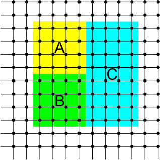
Figure 2: The separation of the system into subsystem $A$, $B$, $C$ and environment, periodic boundary condition is employed in both $\hat{x}$ and $\hat{y}$ directions.

We study system with total dimensions 12 $\times$ 12 lattice spacings in both directions with periodic boundary conditions. We separate the system into $L_{A}\times L_{A}$ squares A and B and an $L_{A}\times 2L_{A}$ rectangle C, see Fig 2. For this particular geometry, TEE is simply given by:

$$-\gamma=2S_{2,A}-2S_{2,AC}+S_{2,ABC}$$ (7)

where we have used the fact that $S_{2,A}=S_{2,B}$, $S_{2,AB}=S_{2,C}$ and $S_{2,AC}=S_{2,BC}$ owing to the reflection and translation symmetry of the wave function. This simplifies the measurement of TEE into the measurement of $S_{2}$ for only three subsystems $A$, $AC$ and $ABC$.

We use the unprojected wave-function as a benchmark for extraction of TEE, which is non-interacting and hence exactly solvable. For an $L_{A}=3$ system, the VMC calculation gives $\gamma=-0.0008\pm 0.0059$, in agreement with the absence of topological order and correspondingly vanishing TEE(table 1 first row).

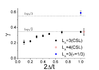
Figure 3: Illustration of finite size effect: chiral SL TEE $\gamma$ as a function of $2\Delta/t$ proportional to the relative gap size for characteristic system length $L_{A}=3$. The larger the gap, the closer the data approaches the ideal value. For comparison, TEE $\gamma$ for chiral SL at $L_{A}=4$ and $2\Delta/t=1.0$ is shown. On the same plot, TEE $\gamma$ of a lattice version of $\nu=1/3$ Laughlin state at $L_{A}=3$, $2\Delta/t=1.0$ is also shown. The dashed lines are the ideal TEE values of $\gamma=\log\left(\sqrt{2}\right)$ for the chiral SL and $\log\left(\sqrt{3}\right)$ for the $\nu=1/3$ Laughlin state.

The Gutzwiller projected wave-function is believed to be a chiral SL which can be thought of as a Laughlin liquid at filling $\nu=1/2$. Using VMC method, we find $\gamma=0.343\pm 0.012$ for an $L_{A}=3$ system and $\gamma=0.344\pm 0.043$ for an $L_{A}=4$ system, both are in excellent consistency with the expectation of $\gamma=\log\left(\sqrt{2}\right)=0.347$ for its ground states’ two fold degeneracy, see table 1 second and third rows and also Fig.3.

We also want to point out that Gutzwiller projection qualitatively changes the system ground state’s topological and quantum behavior from the mean field result.

On the other hand, by lowering the ratio of $2\Delta/t$ and correspondingly the gap size the correlation length increases and the finite size effects from subleading terms become more important. See Fig.3 for the approach of the extracted TEE $\gamma$ to its universal value of $\gamma=\log\left(\sqrt{2}\right)$ as we lift the gap size controlled by $2\Delta/t$ for a system with typical length scale $L_{A}=3$. The finite size analysis and the above consistency between $L_{A}=3,4$ confirm that finite size effect is small for our chosen sets of parameters for the system sizes we study.

IV A Lattice Version of the Laughlin State

Using VMC method, we further study the situations where the wave-function is the cube or the fourth power of the Slater determinant of the Chern insulator. For example, consider the wave-function:

$$\Psi_{1/3}(r_{1},\,r_{2}\dots,\,r_{N})=\Phi^{3}(r_{1},\dots,\,r_{N})$$ (8)

where $\Phi$ is the Chern insulator Slater determinant defined above. Clearly, the product is a fermionic wave-function, since exchanging a pair of particles leads to a sign change. This is similar in spirit to constructing the corresponding Laughlin liquid of $m=3$ of fermions, by taking the cube of the Slater determinant wave-function in the lowest Landau level $\psi(z_{1},\dots,\,z_{N})=\prod_{i<j}(z_{i}-z_{j})e^{-\sum_{i}\frac{|z_{i}|^{2}}{4l^{2}_{B}}}$). However, unlike the canonical Laughlin state, composed of lowest Landau level states, these are rather different lattice wave-functions. An interesting question is whether the lowest Landau level structure is important in constructing states with the topological order of the Laughlin state, or whether bands with identical Chern number is sufficient, as suggested by field theoretic arguments.

To address this we calculate TEE and compare with expectation for the Laughlin phase. Again we choose $L_{A}=3$ in our VMC simulation, and obtain: $\gamma=0.5894\pm 0.0272$ for the $m=3$ wave-function, in reasonable agreement with the ideal value $\gamma=\log\left(\sqrt{3}\right)=0.549$(table 1 fourth row).

We also considered the fourth power of the Chern insulator Slater determinant:

$$\Psi_{1/4}(r_{1},\,r_{2}\dots,\,r_{N})=\Phi^{4}(r_{1},\dots,\,r_{N})$$ (9)

this is a bosonic wave-function, that is expected to be in the same phase as $\nu=1/4$ bosons. Indeed we find with $L_{A}=3$ in our VMC simulation, $\gamma=0.732\pm 0.076$, consistent with ideal value that must be realized in the thermodynamic limit of this phase: $\gamma=\log\left(\sqrt{4}\right)=0.693$(table 1 fifth row).

These results offered direct support for the TEE formula $\gamma=\log D$ as well as their validity as topological ground state wave-functions carrying fractional charge and statistics. The lattice fractional Quantum Hall wave-functions discussed here may be relevant to the recent studies of flat band Hamiltonians with fractional quantum Hall states tang2010 ; sheng2011 .

V Entanglement Entropy of a $Z_{2}$ spin liquid

With the projected wave-function ansatz, we may also construct a topological $Z_{2}$ SL by projecting another mean-field BCS state, given by the specific BdG Hamiltonian on a square lattice as the followingwen2004 :

$$H=-\underset{\left\langle ij\right\rangle}{\sum}\left(\psi_{i}^{\dagger}\mu_{ij}\psi_{j}+h.c.\right)+\underset{i}{\sum}\psi_{i}^{\dagger}a_{0}^{l}\tau^{l}\psi_{i}$$

where $\psi_{i}=\left(f_{\uparrow},f_{\downarrow}^{\dagger}\right)^{T}$. $\tau^{1,2,3}$ are Pauli matrices. The second term is related to chemical potentials, we set $a_{0}^{2,3}=0$, with $a_{0}^{1}$ fixed by the conditions $\left\langle\psi^{\dagger}\tau^{1,2,3}\psi\right\rangle=0$. Matrices $\mu_{ij}$ connecting nearest and next nearest neighbors:

$$\mu_{i,i+x} = \mu_{i,i+y}=-\tau^{3}$$

$$\mu_{i,i+x+y} = \eta\tau^{1}+\lambda\tau^{2}$$

$$\mu_{i,i-x+y} = \eta\tau^{1}-\lambda\tau^{2}$$

This mean field model is readily solvable, with dispersion:

$$E_{k} = \sqrt{\epsilon_{k}^{2}+\left|\Delta_{k}^{2}\right|}$$

$$\epsilon_{k} = 2\left(\cos\left(k_{x}\right)+\cos\left(k_{y}\right)\right)$$

$$\Delta_{k} = 2\eta\left[\cos\left(k_{x}+k_{y}\right)+\cos\left(k_{x}-k_{y}\right)\right]+a_{0}^{1}$$

$$-2i\lambda\left[\cos\left(k_{x}+k_{y}\right)-\cos\left(k_{x}-k_{y}\right)\right]$$

We choose $\eta=\lambda=1.5$ for a large gap and our calculation estimates that the correlation length is as short as $\xi\sim 1.3$ lattice spacings.

The VMC algorithm need little changegros1989 , except that instead of Slater determinants product, the wave-function for spin product configuration $\left|\alpha\right\rangle$ is given by

$$\phi_{\alpha}=\left\langle\alpha|\Phi\right\rangle=\det\left(a_{ij}\right)$$

here $a_{ij}=a\left(r_{i,\uparrow}-r_{j,\downarrow}\right)$ is the Fourier transform of the superconducting pairing function$f_{k}$, $r_{i,\uparrow}$ and $r_{j,\downarrow}$ are the coordinates of the up-spins and down-spins, respectively:

$$f_{k}=\frac{\Delta_{k}}{\left|E_{k}+\epsilon_{k}\right|}$$

For numerical simulations we again study $12\times 12$ lattice spacing systems and separate the system into subsystems including $L_{A}\times L_{A}$ squares $A$ and $B$ and $L_{A}\times 2L_{A}$ rectangle $C$, again see Fig.2. The TEE $\gamma$ is given by Eq.7 as before. First, we use the unprojected BCS state as a benchmark, for which we expect a result of $\gamma=0.003$ from an exact solution (since the unprojected state is a free particle ground state, one may use the correlation matrix methodcorrelation-matrix ) and consistent with its absence of topological order. Indeed, we obtain $\gamma=0.012\pm 0.062$ using VMC method, the almost vanishing value of $\gamma$ is consistent with the expected value, which also serves as a check on our Monte Carlo calculations.

On the other hand, the projection qualitatively alters the topological properties of the system, and for simulation accuracy and efficiency, we employ the ’sign trick’ from Ref.frank2011 . For an $L_{A}=4$ system, the VMC calculation gives $\gamma=0.584\pm 0.089$. This is roughly consistent the $Z_{2}$ SL which has $D^{2}=4$ sectors and $\gamma=\log\left(D\right)=\log\left(2\right)\simeq 0.693$. The TEE is found to be about $84\%$ of the expected value(table 1 last row). Other studies on Z₂ phases eg. the quantum Monte Carlo on a Bose Hubbard model in Ref.isakov2011 have also found values that underestimate the topological entropy ($75\%$ of the expected zero temperature value in that case). The smaller than expected value is probably due to spinon excitations with a finite gap, causing breaking of $Z_{2}$ electric field lines over the finite system size $L_{A}=4$ we consider. Indeed, spin correlations decay more slowly for the $Z_{2}$ state, as compared to the chiral SL, which also arrives closer to its expected $\gamma$ value. Consistent with this fact is the observation that for a smaller system size $L_{A}=3$ where the finite system size has a larger impact, VMC calculation leads to a value of $\gamma=0.446\pm 0.119$, which is further away from the ideal value.

VI Conclusion

In this paper we studied entanglement properties of candidate wave-functions for $SU(2)$ symmetric gapped SLs and Laughlin states, and established their topological order using the notion of TEE. We studied two classes of SLs: 1) Wave-functions that describe quantum Hall states and are obtained from the wave-function of a Chern insulator by taking multiple copies of it 2) A $Z_{2}$ SL state that is obtained by Gutzwiller projecting a fully-gapped BCS superconductor. These wave-functions have long been used as ansatz for exploring SLs states and it is reassuring that topologically ordered states can be good variational ground states for realistic Hamiltonians. Our method is directly applicable to any wave-function that can be dealt within VMC method and would be especially useful in cases where one is dealing with a Hamiltonian that has Monte Carlo sign-problem and only has a variational ansatz for the corresponding ground state. We also note that since the quantum Hall wave-functions we study are not constructed from the lowest Landau level but rather from the band structures that have non-zero Chern number, our results are also relevant to the recently discovered quantum Hall physics in flat band Hamiltonians tang2010 ; sheng2011 .

Let us consider a few problems where our method may find immediate application. Firstly, it would be interesting to apply our method to $Z_{2}$ SLs that have gapless nodal spinons. These SLs are obtained by Gutzwiller projecting a nodal BCS state. We note that in this case one would find an additional contribution to the subleading constant part of the entanglement entropy that comes from the gapless spinons. Though we believe it might still be possible to separate the total contribution of the constant term into a topological constant and a term that comes from the gapless spinons only. It would also be interesting to study wave-functions that are expected to have non-abelian quasi-particles such as $SU(2)_{k}$ quantum Hall wave-functionsronny1 . Thirdly, since VMC techniques can be used for wave-functions defined in the continuum as well, it might be interesting to study TEE of quantum Hall wave-functions (and their descendants such as time-reversal invariant fractionalized topological insulators levin2009 ) defined directly in the continuum.

Finally, we note that one limitation of our method is that it can’t be used to calculate TEE for SLs where the gauge fields are coupled to bosonic (rather than fermionic) spinons. This is because VMC techniques are not very efficient when dealing with wave-functions that are written as permanents (in contrast to determinants). It would be interesting to see if the recent VMC calculation for a $SU(2)$ symmetric bosonic SL tay2011 can be pushed to bigger system sizes so as to establish topological order in such wave-functions.

Acknowledgements: We acknowledge support from NSF DMR- 0645691.

References

- (1) P.W. Anderson, Science 237, 1196 (1987).
- (2) S. Kivelson, D. Rokhsar, J. Sethna, Phys. Rev. B 35, 8865 (1987).
- (3) N. Read, B. Chakraborty, Phys. Rev. B 40, 7133 (1989).
- (4) T. Senthil, A. Vishwanath, L. Balents, S. Sachdev and M. P. A. Fisher, Science 303, 1490 (2004).
- (5) Y. Shimizu, K. Miyagawa, K. Kanoda, M. Maesato, and G. Saito, Phys. Rev. Lett. 91, 107001 (2003); Y. Okamoto, M. Nohara, H. Aruga-Katori and H. Takagi, Phys. Rev. Lett. 99. 137207 (2007); J. S. Helton et al., Phys. Rev. Lett. 98, 107204 (2007); M. Yamashita et al, Science 328, 1246 (2010).
- (6) Simeng Yan, David A. Huse, Steven R. White, Science 332, 1173 (2011).
- (7) Z. Y. Meng, T. C. Lang, S. Wessel, F. F. Assaad, A. Muramatsu, Nature 464, 847 (2010).
- (8) Xiao-Gang Wen, Quantum field theory of many-body systems, Oxford Graduate Texts, 2004.
- (9) A. Hamma, R. Ionicioiu, and P. Zanardi, Phys. Lett. A 337, 22 (2005); Phys. Rev. A 71, 022315 (2005).
- (10) M. Levin, X.-G. Wen, Phys. Rev. Lett. 96, 110405 (2006).
- (11) A. Kitaev, J. Preskill, Phys. Rev. Lett. 96, 110404 (2006).
- (12) D. S. Rokhsar and S. A. Kivelson, Phys. Rev. Lett. 61, 2376 (1988).
- (13) R. Moessner, S. L. Sondhi, Phys. Rev. Lett. 86, 1881 (2001).
- (14) T. Senthil, O. Motrunich, Phys. Rev. B 66, 205104 (2002).
- (15) L. Balents, M.P.A. Fisher, S.M. Girvin, Phys. Rev. B 65, 224412 (2002).
- (16) G. Misguich, D. Serban and V. Pasquier, Phys. Rev. Lett. 89, 137202 (2002).
- (17) N. Read and S. Sachdev, Phys. Rev. Lett. 66, 1773 (1991); S. Sachdev, Physical Review B 45, 12377 (1992).
- (18) S. Furukawa and G. Misguich, Phys. Rev. B 75, 214407 (2007).
- (19) C. Castelnovo and C. Chamon, Phys. Rev. B 76, 174416 (2007).
- (20) S. Papanikolaou, K. S. Raman, and E. Fradkin, Phys. Rev. B 76, 224421 (2007).
- (21) A. Hamma, W. Zhang, S. Haas, and D. A. Lidar, Phys. Rev. B 77, 155111 (2008).
- (22) Sergei V. Isakov, Matthew B. Hastings, Roger G. Melko, arXiv:1102.1721.
- (23) O. I. Motrunich, Phys. Rev. B 72, 045105 (2005); L. F. Tocchio, A. Parola, C. Gros, and F. Becca, Phys. Rev. B 80, 064419 (2009); T. Grover, N. Trivedi, T. Senthil and Patrick A. Lee, Phys. Rev. B 81, 245121 (2010).
- (24) V. Kalmeyer and R. B. Laughlin, Phys. Rev. Lett. 59, 2095; V. Kalmeyer and R. B. Laughlin, Phys. Rev. B 39, 11 879; X. G. Wen, Frank Wilczek, and A. Zee, Phys. Rev. B 39, 11 413 (1989).
- (25) T. Senthil and Matthew P. A. Fisher, Phys. Rev. B 62, 7850 (2000).
- (26) X.-G. Wen, Phys. Rev. B. 44, 2664 (1991).
- (27) Yi Zhang, Tarun Grover, Ashvin Vishwanath, arXiv:1102.0350.
- (28) S. T. Flammia, A. Hamma, T. L. Hughes, and X.-G. Wen, Phys. Rev. Lett. 103, 261601 (2009).
- (29) S. Dong, E. Fradkin, R. G. Leigh and S. Nowling, Journal of High Energy Physics 05 (2008) 016.
- (30) M. Haque, O. Zozulya and K. Schoutens, Phys. Rev. Lett. 98, 060401 (2007); O. S. Zozulya, M. Haque, K. Schoutens, and E. H. Rezayi, Phys. Rev. B 76, 125310 (2007); A. M. Lauchli, E. J. Bergholtz and M. Haque, New J. Phys. 12, 075004 (2010).
- (31) D. A. Ivanov, T. Senthil, Phys. Rev. B 66, 115111 (2002). A. Paramekanti, M. Randeria and N. Trivedi, Phys. Rev. B 71, 094421 (2005).
- (32) Hong Yao and Xiao-Liang Qi, Phys. Rev. Lett. 105, 080501 (2010).
- (33) H. Li and F. D. M. Haldane, Phys. Rev. Lett. 101, 010504 (2008).
- (34) A. Kitaev, Ann. Phys., 303, 2 (2003).
- (35) M. B. Hastings, I. Gonzalez, A. B. Kallin and R. G. Melko, Phys. Rev. Lett. 104, 157201 (2010).
- (36) C. Gros, Annals of Physics 189, 53 (1989).
- (37) D. F. Schroeter, E. Kapit, R. Thomale, and M. Greiter, Phys. Rev. Lett. 99, 097202 (2007).
- (38) A. W. W. Ludwig, M. P. A. Fisher, R. Shankar, G. Grinstein, Phys. Rev. B 50, 7526 (1994).
- (39) E. Tang, J.-W. Mei, and X.-G. Wen, Phys. Rev. Lett. 106, 236802 (2011). T. Neupert, L. Santos, C. Chamon, and C. Mudry, Phys. Rev. Lett. 106, 236804 (2011); K. Sun, Z. C. Gu, H. Katsura, and S. Das Sarma, Phys. Rev. Lett. 106, 236803 (2011).
- (40) Y.-F. Wang, Z. C. Gu, C.-D. Gong, D. N. Sheng, arXiv:1103.1686; D. N. Sheng, Z. C. Gu, K. Sun, L. Sheng, Nature Communications 2, 389 (2011); N. Regnault, B. A. Bernevig, arXiv:1105.4867.
- (41) I. Peschel, V. Eisler, J. Phys. A: Math. Theor. 42, 504003 (2009).
- (42) B. Scharfenberger, R. Thomale, M. Greiter, arXiv:1105.4348.
- (43) M. Levin and A. Stern, Phys. Rev. Lett. 103, 196803 (2009).
- (44) Tiamhock Tay, Olexei I. Motrunich, Phys. Rev. B 84, 020404(R) (2011).