Supersolid phase transitions for hardcore bosons on a triangular lattice

Abstract

Hard-core bosons on a triangular lattice with nearest neighbor repulsion are a prototypical example of a system with supersolid behavior on a lattice. We show that in this model the physical origin of the supersolid phase can be understood quantitatively and analytically by constructing quasiparticle excitations of defects that are moving on an ordered background. The location of the solid to supersolid phase transition line is predicted from the effective model for both positive and negative (frustrated) hopping parameters. For positive hopping parameters the calculations agree very accurately with numerical quantum Monte Carlo simulations. The numerical results indicate that the supersolid to superfluid transition is first order.

I Introduction

A supersolid is characterized by a non-trivial solid order parameter which co-exists with an off-diagonal long-range superfluid order parameter.supersolid1 This state appears counter-intuitive since the superfluid density implies ballistic coherent transport without disturbing the ordered background of the solid. The possibility of a supersolid was discussed in the early 1970’s and since then much attention has been focused on ⁴He as the most likely experimental realization, which remains controversial.supersolid_experiment1 The motions of many different kinds of defects have been considered as possible mechanisms for supersolidity in ⁴He, including vacancies,supersolid1 grain boundaries grain_boundary or dislocations dislocation which may be able to move through a solid state. In recent years supersolid behavior on lattices has been established theoretically in a number of interacting boson models,wess ; tri2 ; tri4 ; tri6 ; tri7 ; tri8 ; tri9 ; imp which now gives hope for an experimental realization of a supersolid with the help of ultra-cold gases.sengstock One prototypical example to exhibit a supersolid phase are hard-core bosons with nearest neighbor repulsion on a triangular lattice GL ; wess ; tri2 ; tri4 ; tri6 ; tri7 ; tri8 ; tri9 which are described by the Hamiltonian

$$H_{0} = -t\mathop{\sum}_{\langle ij\rangle}(b_{i}^{{\dagger}}b_{j}+b_{j}^{{\dagger}}b_{i})+V\mathop{\sum}_{\langle ij\rangle}n_{i}n_{j}-\mu\mathop{\sum}_{i}n_{i},$$ (1)

where $b_{i}^{{\dagger}}$ $(b_{i})$ is the boson creation (annihilation) operator, $t$ describes the hopping amplitude, $\mu$ is the chemical potential, $V$ reflects the repulsion effect, and $\langle i,j\rangle$ represents nearest-neighbor sites.

For positive hopping $t>0$ a supersolid phase has been shown using numerical simulations wess ; tri2 ; tri4 and variational wavefunctions.tri6 ; tri7 For negative hopping $t<0$ it is not possible to use quantum Monte Carlo (QMC) simulations, but at least for the special case of half filling a supersolid phase has been confirmed.tri8 ; tri9 While the existence of the supersolid phase has been firmly established in this model, it would be desirable to obtain a better understanding of the physical mechanism leading to the supersolid phase and an analytical description of the quantum phase transition.

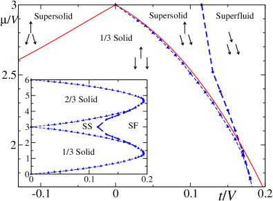
Figure 1: The phase diagram of hard-core bosons on the triangular lattice. The dashed lines (blue) are numerical QMC results while the solid lines (red) are the analytical results from Eqs. (3) and (4). The arrows indicate the order in terms of the classical directions in the spin-wave theory. Inset: Overview of the entire particle-hole symmetric region.

The phase diagram of the model is shown in Fig. 1. For $0<\mu<3V$ and $t=0$ the solid order is described by a 1/3-ordered state, where the unoccupied sites form a honeycomb sublattice around the filled sites as indicated in Fig. 2. Due to particle-hole symmetry the equivalent behavior can be seen for $\mu/V>3$ in the form of a 2/3 filled state (see inset of Fig. 1). The goal of this paper is an analytic quantitative description of the transition to the supersolid phase which occurs for $t\neq 0$ around $\mu/V=3$. The solid order is three-fold degenerate according to the choice of sublattice, however this degeneracy is not important for the formation of the supersolid state so we will only consider one representative $1/3$-filled state in what follows. Finite hopping $t\neq 0$ causes quantum fluctuations in form of virtual excitations from the occupied sites onto the unoccupied ones and back. Therefore the ordered state is renormalized, e.g. the density of the unoccupied honeycomb lattice is now finite $\sim 3t^{2}/4V^{2}$ to lowest order and the occupied density is reduced $\sim 1-3t^{2}/2V^{2}$. However, the delocalization of these virtual excitations is not the driving mechanism for the transition into the supersolid state. Instead we conjecture that a different type of excitation starts to appear at the phase transition, namely ”defects” consisting of additional occupied sites. These defects can only move on the honeycomb lattice of unoccupied sites, while the solid order remains surprisingly stable, which leads to an effective model.

II Effective model

The corresponding effective Hamiltonian for hard-core boson defects on the honeycomb lattice can be derived in the strong coupling expansion. Ordinary perturbation theory has a diverging number of contributions, but it is possible to analyze the movement of a single defect by only taking those terms into account which actually involve the defect.schmidt This results in the following effective Hamiltonian on the honeycomb sublattice

$$H_{\rm eff}=-\sum_{i,d}\tilde{t}_{d}(a_{i}^{\dagger}a_{i+d}^{\phantom{\dagger}}+a_{i+d}^{\dagger}a_{i}^{\phantom{\dagger}})+V\mathop{\sum}_{\langle ij\rangle}m_{i}m_{j}-\tilde{\mu}\sum_{i}m_{j},$$ (2)

where $m_{i}=a_{i}^{\dagger}a_{i}^{\phantom{\dagger}}$ and the effective hopping parameters are given by $\tilde{t}_{1}=t+t^{2}/V$ for nearest neighbors, $\tilde{t}_{2}=t^{2}/V$ for next nearest neighbors, and $\tilde{t}_{3}=t^{2}/V$ for next-next nearest neighbors on the honeycomb sublattice as shown in Fig. 2. The second-order terms arise from a two-step hopping process, where a boson from the occupied sublattice jumps on an unoccupied site and then the defect takes the place of the original boson, thereby effectively transporting the defect. Likewise, the effective chemical potential is changed $\tilde{\mu}=\mu-3V+5t^{2}/2V$ since virtual excitations from the unoccupied sublattice and back are now affected by the defect, which results in an effective self-energy. Since the defects can move ballistically and coherently on the unoccupied honeycomb sublattice according to the effective model, a finite density of such defects also explains the coexistence of a finite superfluid density on top of a relatively stable renormalized ordered state, which are in fact the central characteristics of the supersolid phase.

The effective model in Eq. (2) is of course still an interacting hard-core boson model, but is much easier to treat since we only have to consider small densities of defects as will be seen below. In particular, according to our hypothesis the phase transition line is simply determined by the point when it is energetically favorable to create one single defect. For positive hopping $t>0$ the energy of a single defect is minimized in the uniform $k=0$ state with a total energy of $\tilde{E}_{+}=-3\tilde{t}_{1}-6\tilde{t}_{2}-3\tilde{t}_{3}-\tilde{\mu}$, which must change sign at the phase transition line. By taking also third order processes into account this results in the following prediction for the phase transition line between solid and supersolid

$$\mu_{+} = 3V-3t-\frac{29t^{2}}{2V}-\frac{77t^{3}}{4V^{2}}+{\cal{O}}(t^{4}).$$ (3)

As shown in Fig. 1 this result agrees remarkably well with our QMC simulations, where we used the stochastic series expansion with parallel tempering.sse1 The errorbars for the data from the QMC simulations are smaller than the size of the symbols in all figures. For $\mu>3V$ the particle hole symmetric line is given by $\tilde{\mu}_{+}=6V-\mu_{+}$.

A similar analysis can be made for negative hopping $t<0$. Since the honeycomb lattice is bi-partite the positive nearest neighbor hopping can be restored by a simple Gauge transformation of $-1$ on one sublattice, but the next-nearest neighbor coupling remains negative. Therefore, the ground state energy of one defect is now $\tilde{E}_{-}=3\tilde{t}_{1}-6\tilde{t}_{2}+3\tilde{t}_{3}-\tilde{\mu}$, and accordingly we obtain a phase transition line of the form

$$\mu_{-} = 3V+3t-\frac{5t^{2}}{2V}-\frac{71t^{3}}{4V^{2}}+{\cal{O}}(t^{4}),$$ (4)

where we have again taken third order processes into account. For negative hopping it is more difficult to treat the problem with numerical methods, so there are no independent checks for this prediction so far. However, considering the good agreement for the positive hopping case above, it is reasonable to expect that the same calculation also applies for negative hopping with similar accuracy. We therefore find that the supersolid region is stable but slightly narrower for negative hopping, which appears to be caused by the additional kinetic frustration.

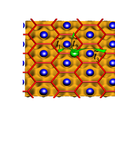
Figure 2: Schematic description of the effective model on the unoccupied honeycomb sublattice (lines) where the defect (large central sphere) can hop to neighboring sites. Smaller spheres (blue) are occupied sites, which only participate in virtual excitations.

III analytical and numerical results near the phase transition

In order to calculate the detailed behavior near the phase transition analytically it is now possible to use linear spin-wave theory on the effective Hamiltonian in Eq. (2). It should be noted that the system is at low filling (i.e. nearly saturated in terms of spins) and that the honeycomb lattice has two nonequivalent sites, but otherwise the spin-wave calculation follows the standard scheme.Weihong In particular, the hard-core bosons can be mapped exactly onto spins, which are expressed in a rotated frame according to the classical alignment. The classical angle relative to the $z$-direction is given by $\cos\theta=B/(3V/2-\sum_{d}\tilde{t}_{d}$) in terms of the field $B=\tilde{\mu}-3V$. The spins are then re-expressed in terms of regular bosons, which has the advantage that the interaction can be solved by a Bogoluibov transformation to linear order. This procedure is especially reliable in the low density limit near the phase transition that we are interested in. The details of this calculation can be found in the appendix. The density $\langle\rho\rangle=\frac{1}{2}-\langle S^{z}\rangle$ on the honeycomb sublattice at $T=0$ is then given in terms of the Bogoluibov rotation angles

$$\langle\rho\rangle=\frac{1}{2}-\cos\theta\left[\frac{1}{2}-\frac{2}{N}\sum_{k}\left(\sinh^{2}\theta_{k}^{\alpha}+\sinh^{2}\theta_{k}^{\beta}\right)\right],$$ (5)

where	$\tanh 2\theta_{k}^{\alpha}=-|\gamma_{k}|A/\left(t+|\gamma_{k}|\left(A-t\right)\right)$
and	$\tanh 2\theta_{k}^{\beta}=-|\gamma_{k}|A/\left(t-|\gamma_{k}|\left(A-t\right)\right)$
with	$A=\sin^{2}\theta\left(2t+V\right)/4$ and
$|\gamma_{k}|=$	$\frac{1}{3}\left[3+4\cos\frac{3k_{x}}{2}\cos\frac{\sqrt{3}k_{y}}{2}+2\cos\left(\sqrt{3}k_{y}\right)\right]^{1/2}$.

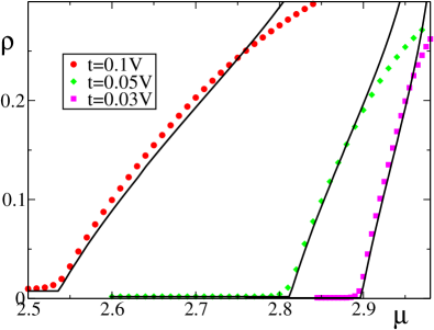
Figure 3: The density on the sites with lower filling on the triangular lattice near the phase transition (symbols) for $t=0.03V$ ($V\beta=300$), $t=0.05V$ ($V\beta=150$) and $t=0.1V$ ($V\beta=100$). The solid lines are the analytical prediction from Eq. (5).

In Fig. 3 we show the density on the unoccupied sublattice from QMC simulations on a triangular lattice with $24^{2}$ sites near the solid to supersolid phase transition at different hoppings (symbols). This can be compared to the spin-wave results for the density on the honeycomb lattice from Eq. (5) (lines), where the small background contribution $3t^{2}/4V^{2}$ from virtual excitations was added. The virtual excitations are localized so this finite background density does not contribute to the superfluid density which is also confirmed by the data in Fig. 4. Here and in what follows the spin-wave results always include the additional third order shift in $\mu$ by $77t^{3}/4V^{2}$ from Eq. (3). The good agreement not only confirms the validity of the effective model on the honeycomb lattice in Eq. (2), but also provides an analytical tool to calculate the general behavior and correlations near the phase transition for both positive and negative hopping $t$. As a check we have also computed densities and correlations on the honeycomb lattice, which agree equally well with the original triangular model (not shown). The correlations between the occupied sublattice and the unoccupied honeycomb sublattice can be calculated by the modified perturbation theory discussed above, which results in positive $\langle b^{\dagger}_{i}b_{j}\rangle$ correlations between sublattices for $t>0$, while the correlations cancel to second order for $t<0$, i.e. the occupied sublattice always gives only a very weak contribution to the superfluid density as indicated by the spin directions in Fig. 1.

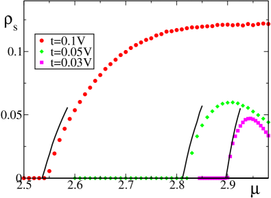
Figure 4: The superfluid density on the triangular lattice near the phase transition (symbols). The solid lines are the analytical prediction from Eq. (6).

The superfluid density on the unoccupied honeycomb sublattice can be calculated in the effective spin model as the response to a small twist $\nu$ in the x-y plane $\rho_{s}=d^{2}\langle H(\nu)\rangle/d^{2}\nu$. Expanding the Hamiltonian leads to $H(\nu)=H+\sum_{i,d}\left(\nu_{d}J^{s}_{d}+\nu_{d}^{2}/2T_{d}\right)$, where $\nu_{d}$ is the projection of the twist along the corresponding bond direction, $J^{s}_{d}=(i/2)\widetilde{t}_{d}\left(S_{i}^{+}S_{i+d}^{-}-S_{i+d}^{+}S_{i}^{-}\right)$ is the spin current, and $T_{d}=(1/2)\widetilde{t}_{d}\left(S_{i}^{+}S_{i+d}^{-}+S_{i+d}^{+}S_{i}^{-}\right)$ is the spin-kinetic energy.Schulz ; Cuccoli In linear spin-wave theory the response to the spin current does not contribute in the low density limit and the superfluid is therefore approximated by the correlation functions $T_{d}$ of neighbors connected by $\tilde{t}_{d}$

$$\rho_{s}\approx\frac{1}{2}(T_{1}+4T_{2}+3T_{3})$$ (6)

which can be calculated in the rotated spin frame (see appendix). In Fig. 4 we compare the results from Eq. (6) on the honeycomb lattice with the superfluid density $\rho_{s}$ derived from the winding number $\langle W^{2}\rangle/4\beta t$ in QMC simulations for the triangular lattice in the thermodynamic limit near the phase transition. The predictions from the effective model also show a sharp increase at the phase transition, but the agreement is limited to a smaller region since the contribution of the spin current response was not included. In any case, the agreement near the phase transition line again gives strong support for the validity of the effective model in Eq. (2).

IV Analysis of the phase transition

Finally, we would like to consider the implications of our model for the supersolid to superfluid transition, which has been reported to be second order before.wess If our model is correct this transition should simply correspond to a melting of the solid due to the appearance of more and more virtual excitations, i.e. a breakdown of the perturbation expansion. While we have not found an energetic condition which would quantify the location of the supersolid to superfluid transition line, we believe that such a melting transition should be first order. One reason is also that a third order term in the Ginzburg Landau expansion is generically allowed by momentum conservation for an order parameter with triangular symmetry, so that a continuous transition can only occur at special points.rosch We have therefore tested the behavior of the phase transition with QMC simulations. In Fig. 5 it can be seen that for $t=0.16$ the structure factor abruptly goes to zero close to $\mu=2.012(2)$ while the densities show clear discontinuities. For larger $\mu$ and smaller $t$ closer to the particle-hole symmetric point these discontinuities become systematically smaller, but can still be observed even without histogram methods. The discontinuity in $\rho$ corresponds to a region of phase separation if the density is held fixed as shown in the inset. During preparation of the paper we discussed our discovery of the first order behavior with one of the authors of Ref. [wess, ] and since then two quantitative studies have appeared which confirm the first order behavior.wessnew

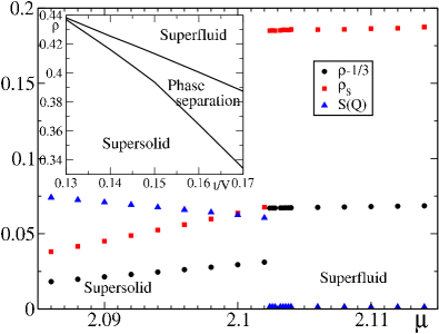
Figure 5: The density, structure factor $S(Q)=\langle|\mathop{\sum}_{r}\hat{S}^{z}_{r}e^{iQ\cdot r}|^{2}\rangle/N^{2}$ at $Q=\!\![4/3\pi,0]$ and the superfluid density with $L=36$ and $T=0.01$ at $t=0.16$ and $V=1$ by varying $\mu$. Inset: Observed region of phase separation between supersolid and superfluid phases.

V Conclusions

In conclusion we proposed an analytical model in the form of defects moving in an ordered background, which gives a quantitative description of the solid to supersolid transition in the hard-core boson model. In this way the transition line can be determined and correlations nearby can be calculated with the help of spin-wave theory for positive and negative hopping $t$. For positive $t$ the calculations agree well with QMC simulations. For $t<0$ we make a quantitative prediction for the supersolid region, which has so far not been estimated by numerical methods. We find that the kinetic frustration for $t<0$ does not destroy the supersolid phase, but the higher order corrections imply a narrower region. In fact, the higher order terms imply a possible maximum of the extent of the supersolid phase with increasing $|t|$ in this case. It is indeed feasible that a configuration corresponding to a low density (spin down) on one sublattice and a small x-y antiferromagnetic order on the other two sublattices may be stable all the way to the SU(2) invariant point $V=-2t=\mu/3$. In this case the SU(2) invariant point would play the role of a trivial ”degenerate” supersolid where a superposition of broken orders is possible in any direction.

*

Appendix A Spin wave analysis

We consider a two dimensional system of hardcore bosons on an effective hexagonal lattice in Eq. (2). To enforce the hardcore constraint in a simple way, the Hamiltonian is mapped onto the two dimensional XXZ model with external magnetic field using $a_{i}^{\dagger}\leftrightarrow S_{i}^{+}$, $a_{i}\leftrightarrow S_{i}^{-}$, and ${\hat{n}_{i}}\leftrightarrow S_{i}^{z}+1/2$. With this mapping the hardcore boson model becomes

$$H=-\sum_{i,d}\widetilde{t}_{d}(S_{i}^{+}S_{j}^{-}+S_{i}^{-}S_{j}^{+})+\sum_{\langle ij\rangle}VS_{i}^{z}S_{j}^{z}-B\sum_{i}S_{i}^{z}$$ (7)

where $B=\widetilde{\mu}-\lambda V$ is an effective field and $\lambda=3/2$ is half the coordination number on a hexagonal lattice. Here and in what follows we generally omit the ground state energy.

The $z$-axis can be aligned with the mean field magnetization direction by the rotation $S_{i}^{x}=S_{i}^{\prime x}{\rm cos}(\theta)+S_{i}^{\prime z}{\rm sin}(\theta)$, $S_{i}^{y}=S_{i}^{\prime y}$ and $S_{i}^{z}=-S_{i}^{\prime x}{\rm sin}(\theta)+S_{i}^{\prime z}{\rm cos}(\theta)$, where ${\vec{S}}_{i}^{\prime}$ is the spin vector in the rotated frame. The hexagonal lattice has two spins per unit cell, which are are expressed in terms of bosonic operators $c_{i}$ ($c_{i}^{\dagger}$) and $d_{i}$ ($d_{i}^{\dagger}$) respectively, i.e. $S_{i}^{\prime x}=\frac{1}{2}(S_{i}^{\prime+}+S_{i}^{\prime-})=\frac{1}{2}(c_{i}^{\dagger}+c_{i})$, $S_{i}^{\prime y}=\frac{1}{2i}(S_{i}^{\prime+}-S_{i}^{\prime-})=\frac{1}{2{\rm i}}(c_{i}^{\dagger}-c_{i})$, $S_{i}^{\prime z}=\frac{1}{2}-c_{i}^{\dagger}c_{i}$ and likewise for the other sublattice in terms of $d_{i}$ ($d_{i}^{\dagger}$). Note that the spin-wave operators obey the usual (soft-core) bosonic commutation relations. Substituting these expressions into Eq. (7) and assuming a dilute gas of spin-waves, we can ignore cubic and quartic terms in the bosonic operators. The linear term in the operators is required to vanish yielding, $\cos\theta=\left(\widetilde{\mu}-\lambda V\right)/\left(\lambda V+\sum_{d}\widetilde{t}_{d}\right)$, where the sum runs over the nearest, next-nearest and next-next-nearest neighbor bonds. The longer range hopping terms of order $t^{2}$ play an important role in determining the mean field angle and the superfluid density below, but they can be neglected when determining the Bogoluibov rotation. Therefore, the Hamiltonian reduces to

$$H = \sum_{<ij>}\left\{A\left(c_{i}^{\dagger}d_{j}^{\dagger}+c_{i}d_{j}\right)+\left(A-t\right)\left(c_{i}^{\dagger}d_{j}+c_{i}d_{j}^{\dagger}\right)\right\}$$ (8)

$$+3t\left(\sum_{i\in A}c_{i}^{\dagger}c_{i}+\sum_{i\in A}d_{i}^{\dagger}d_{i}\right)+H_{MF},$$

where $A=\sin^{2}\theta\left(2t+V\right)/4$ and the mean-field Hamiltonian is given by

$$H_{MF}=N\left[\frac{\cos^{2}\theta}{4}\left(\lambda V+\sum_{d}\tilde{t}_{d}\right)-\frac{\cos\theta}{2}B\right],$$ (9)

which is minimized by the same classical condition $\cos\theta=B/\left(\lambda V+\sum_{d}\widetilde{t}_{d}\right)$. Here $N$ is the total number of lattice sites.

The Hamiltonian (8) can be diagonalized by the Fourier transformation $c_{i}=\sqrt{2/{N}}\sum_{k}e^{i\vec{k}.\vec{r}_{i}}c_{k}$ and $d_{i}=\sqrt{2/{N}}\sum_{k}e^{i\vec{k}.\vec{r}_{i}}c_{k}$. We introduce the structure factor $\gamma_{k}=\frac{1}{3}\sum_{d}e^{i\vec{k}.\vec{r}_{d}}=|\gamma_{k}|e^{i\phi_{k}}$ which is a complex number. The phase $\phi_{k}$ can be absorbed in a gauge transformation $d_{k}\rightarrow e^{-i\phi_{k}}d_{k}$ in the Fourier transformed Hamiltonian and the amplitude of the structure factor reads $|\gamma_{k}|=\frac{1}{3}\left[3+4\cos\frac{3k_{x}}{2}\cos\frac{\sqrt{3}k_{y}}{2}+2\cos\left(\sqrt{3}k_{y}\right)\right]^{1/2}$. The Hamiltonian can be diagonalized using the Bogoluibov transformation Weihong

$$c_{k} = u^{\alpha}_{k}\alpha_{k}+v^{\alpha}_{k}\alpha^{\dagger}_{-k}+u^{\beta}_{k}\beta_{k}-v^{\beta}_{k}\beta^{\dagger}_{-k}$$

$$d_{k} = u^{\alpha}_{k}\alpha_{k}+v^{\alpha}_{k}\alpha^{\dagger}_{-k}-u^{\beta}_{k}\beta_{k}+v^{\beta}_{k}\beta^{\dagger}_{-k}$$

where $u^{\alpha}_{k}=\cosh\theta^{\alpha}_{k}$, $v^{\alpha}_{k}=\sinh\theta^{\alpha}_{k}$, $u^{\beta}_{k}=\cosh\theta^{\beta}_{k}$, and $v^{\beta}_{k}=\sinh\theta^{\beta}_{k}$, with $\tanh{2\theta^{\alpha}_{k}}=-|\gamma_{k}|A/\left(t+|\gamma_{k}|\left(A-t\right)\right)$ and $\tanh{2\theta^{\beta}_{k}}=-|\gamma_{k}|A/\left(t-|\gamma_{k}|\left(A-t\right)\right)$. Finally, the Hamiltonian (8) takes the diagonal form

$$H=\sum_{k}\omega_{k}^{\alpha}\left(\alpha^{\dagger}_{k}\alpha_{k}+1/2\right)+\sum_{k}\omega_{k}^{\beta}\left(\beta^{\dagger}_{k}\beta_{k}+1/2\right).$$ (10)

with $\omega_{k}^{\alpha}=6\sqrt{(t+|\gamma_{k}|(A-t))^{2}-(A|\gamma_{k}|)^{2}}$ and $\omega_{k}^{\beta}=6\sqrt{(t-|\gamma_{k}|(A-t))^{2}-(A|\gamma_{k}|)^{2}}$.

The boson density of the model in Eq. (2) is directly given by $\rho=\left(\langle S^{z}\rangle+1/2\right)$ where the magnetization reads

$$\langle S^{z}\rangle = \langle-S_{i}^{\prime x}\sin\theta+S_{i}^{\prime z}\cos\theta\rangle$$

$$= \cos\theta\left[\frac{1}{2}-\frac{2}{{N}}\sum_{k}\left((v^{\alpha}_{k})^{2}+(v^{\beta}_{k})^{2}\right)\right].$$

which follows from a straight-forward evaluation of the expectation values in terms of the diagonal bosons in Eq. (10).

The superfluid density is given by the second derivative of the energy of the spin system with respect to a uniform twist $\nu$ across the system $\rho_{s}=d^{2}\langle H(\nu)\rangle/d^{2}\nu$. The Hamiltonian $H(\nu)$ is derived from the XXZ model in Eq.(7) by application of a site dependent rotation by an angle $\nu_{i}$ around the $z$ axis, $S_{i}^{+}\rightarrow S_{i}^{+}e^{i\nu_{i}}$, $S_{i}^{-}\rightarrow S_{i}^{-}e^{-i\nu_{i}}$ and $S_{i}^{z}\rightarrow S_{i}^{z}$. Expanding the Hamiltonian around $\nu_{d}=\nu_{i}-\nu_{i+d}=0$ leads to $H(\nu)=H+\sum_{i,d}\left(\nu_{d}J^{s}_{d}+\nu_{d}^{2}/2T_{d}\right)$, where $J^{s}_{d}=(i/2)\widetilde{t}_{d}\left(S_{i}^{+}S_{i+d}^{-}-S_{i+d}^{+}S_{i}^{-}\right)$ is the spin current and $T_{d}=(1/2)\widetilde{t}_{d}\left(S_{i}^{+}S_{i+d}^{-}+S_{i+d}^{+}S_{i}^{-}\right)$ is the spin-kinetic energy.Schulz ; Cuccoli To first-order in perturbation theory the spin stiffness is given by $\rho_{s}=\frac{1}{2N}\frac{\partial^{2}}{\partial\nu^{2}}\sum_{i,d}\nu_{d}^{2}\langle T_{d}\rangle$. Second order perturbation leads to a term integrating the current-current correlator with respect to $J_{s}$, which can be neglected in our spin-wave approach.Cuccoli To obtain the spin stiffness a uniform twist $\nu$ along one direction is applied, which leads to

$$\rho_{s} = \frac{1}{2N}\sum_{i,d}\left(\frac{\partial^{2}}{\partial\nu^{2}}\nu_{d}^{2}\right)\widetilde{t}_{d}\langle S_{i}^{x}S_{i+d}^{x}+S_{i+d}^{y}S_{i}^{y}\rangle,$$ (11)

$$= \frac{\widetilde{t}_{1}}{2}\langle S_{i}^{x}S_{i+1}^{x}+S_{i+1}^{y}S_{i}^{y}\rangle+2\widetilde{t}_{2}\langle S_{i}^{x}S_{i+2}^{x}+S_{i+2}^{y}S_{i}^{y}\rangle$$

$$+\frac{3\widetilde{t}_{3}}{2}\langle S_{i}^{x}S_{i+3}^{x}+S_{i+3}^{y}S_{i}^{y}\rangle,$$

The spin-spin correlation functions are provided by $\langle S_{i}^{x}S_{j}^{x}+S_{j}^{y}S_{i}^{y}\rangle=\cos^{2}\theta\langle S_{i}^{\prime x}S_{j}^{\prime x}\rangle+\sin^{2}\theta\langle S_{i}^{\prime z}S_{j}^{\prime z}\rangle+\langle S_{i}^{\prime y}S_{j}^{\prime y}\rangle$, where $d=1,2,3$ denote nearest neighbor, next-nearest neighbor, and next-next-nearest neighbor, respectively. The spin-spin correlation functions in the rotated frame read

$$\langle S_{i}^{\prime x}S_{i+d}^{\prime x}\rangle = \frac{2}{N}\sum_{k}f_{d}(\vec{k})\Big{(}(v^{\alpha}_{k})^{2}+u^{\alpha}_{k}v^{\alpha}_{k}-(v^{\beta}_{k})^{2}+u^{\beta}_{k}v^{\beta}_{k}\Big{)},$$

$$\langle S_{i}^{\prime y}S_{i+d}^{\prime y}\rangle = \frac{2}{N}\sum_{k}f_{d}(\vec{k})\Big{(}(v^{\alpha}_{k})^{2}-u^{\alpha}_{k}v^{\alpha}_{k}-(v^{\beta}_{k})^{2}-u^{\beta}_{k}v^{\beta}_{k}\Big{)},$$

$$\langle S_{i}^{\prime z}S_{i+d}^{\prime z}\rangle = \left(\langle S^{\prime z}\rangle-1/4\right),\forall d,$$

and the functions $f_{d}(\vec{k})$ are given by

$$f_{1}(\vec{k}) = 2|\gamma_{k}|,$$

$$f_{2}(\vec{k}) = 3|\gamma_{k}|^{2}-1$$

$$f_{3}(\vec{k}) = 2|\gamma_{k}|+\frac{2}{9|\gamma_{k}|}\Big{(}-3+\cos(3k_{x})$$

$$+2\cos(3k_{x}/2)\cos(3\sqrt{3}k_{y}/2)\Big{)}.$$

References

- (1) G.V. Chester, Phys. Rev. A 2, 256 (1970); A.F. Andreev and I.M. Lifshitz, Sov. Phys. JETP 29, 1107 (1969).
- (2) E. Kim and M.H.W. Chan, Nature 427, 225 (2004); Science 305, 1941 (2004).
- (3) S. Sasaki, R. Ishiguro, F. Caupin, H.J. Maris, and S. Balibar, Science 313, 1098 (2006). A. Aftalion, X. Blanc, and R.L. Jerrard, Phys. Rev. Lett. 99, 135301 (2007).
- (4) S.T. Chui, Phys. Rev. B 82, 014519 (2010) R. Pessoa, S.A. Vitiello, and M. de Koning, Phys. Rev. Lett. 104, 085301 (2010)
- (5) S. Wessel and M. Troyer, Phys. Rev. Lett. 95, 127205 (2005).
- (6) D. Heidarian and K. Damle, Phys. Rev. Lett. 95, 127206 (2005). R.G. Melko et al., Phys. Rev. Lett. 95, 127207 (2005).
- (7) M. Boninsegni and N. Prokof’ev, Phys. Rev. Lett. 95, 237204 (2005).
- (8) A. Sen, P. Dutt, K. Damle, and R. Moessner, Phys. Rev. Lett. 100, 147204 (2008).
- (9) F. Wang, F. Pollmann, and A. Vishwanath, Phys. Rev. Lett. 102, 017203 (2009).
- (10) H.C. Jiang et al., Phys. Rev. B 79, 020409(R) (2009).
- (11) D. Heidarian and A. Paramekanti, Phys. Rev. Lett. 104, 015301 (2010).
- (12) X.F. Zhang, Y.C. Wen and S. Eggert Phys. Rev. B 82, 220501(R) (2010).
- (13) C. Becker, et al., New J. Phys. 12, 065025 (2010).
- (14) A.V. Balatsky and E. Abrahams J. Supercond. Nov. Magn. 19, 395 (2006)
- (15) B. Schmidt, et al., Phys. Rev. A 79, 063634 (2009).
- (16) A.W. Sandvik, Phys. Rev. B 59, R14157 (1999); O.F. Syljuåsen and A.W. Sandvik, Phys. Rev. E 66, 046701 (2002).
- (17) Z. Weihong, J. Oitmaa, C.J. Hamer, Phys. Rev. B 44, 11869 (1991); S. Shinkevich, O.F. Syljuåsen, and S. Eggert Phys. Rev. B 83, 054423 (2011).
- (18) T. Einarsson and H.J. Schulz, Phys. Rev. B 51, 6151 (1995).
- (19) A. Cuccoli, T. Roscilde, V. Tognetti, R. Vaia, P. Verrucchi, Phys. Rev. B 67, 104414 (2003).
- (20) A. Rosch, private communication.
- (21) L. Bonnes and S. Wessel, Phys. Rev. B 84, 054510 (2011). D. Yamamoto, I. Danshita, C.A.R. Sa de Melo, preprint arXiv:1102.1317.