Prototype selection for parameter estimation in complex models

Abstract

Parameter estimation in astrophysics often requires the use of complex physical models. In this paper we study the problem of estimating the parameters that describe star formation history (SFH) in galaxies. Here, high-dimensional spectral data from galaxies are appropriately modeled as linear combinations of physical components, called simple stellar populations (SSPs), plus some nonlinear distortions. Theoretical data for each SSP is produced for a fixed parameter vector via computer modeling. Though the parameters that define each SSP are continuous, optimizing the signal model over a large set of SSPs on a fine parameter grid is computationally infeasible and inefficient. The goal of this study is to estimate the set of parameters that describes the SFH of each galaxy. These target parameters, such as the average ages and chemical compositions of the galaxy’s stellar populations, are derived from the SSP parameters and the component weights in the signal model. Here, we introduce a principled approach of choosing a small basis of SSP prototypes for SFH parameter estimation. The basic idea is to quantize the vector space and effective support of the model components. In addition to greater computational efficiency, we achieve better estimates of the SFH target parameters. In simulations, our proposed quantization method obtains a substantial improvement in estimating the target parameters over the common method of employing a parameter grid. Sparse coding techniques are not appropriate for this problem without proper constraints, while constrained sparse coding methods perform poorly for parameter estimation because their objective is signal reconstruction, not estimation of the target parameters.

abstract width 297pt

T3Part of this work was performed in the CDI-sponsored Center for Time Domain Informatics (http://cftd.info).

, , and

t1Supported by a Cyber-Enabled Discovery and Innovation (CDI) Grant 0941742 from the National Science Foundation. t2Supported by ONR Grant 00424143, NSF Grant 0707059 and NASA AISR Grant NNX09AK59G.

1 Introduction

In astronomy and cosmology one is often challenged by the complexity of the relationship between the physical parameters to be estimated and the distribution of the observed data. In a typical application the mapping from the parameter space to the observed data space is built on sophisticated physical theory or simulation models or both. These scientifically motivated models are growing ever more complex and nuanced as a result of both increased computing power and improved understanding of the underlying physical processes. At the same time, data are progressively more abundant and of higher dimensionality as a result of more sophisticated detectors and greater data collection capacity. These challenges create opportunities for statisticians to make a large impact in these fields.

In this paper we address one such challenge in the field of astrophysics. Informally, the setup can be described as follows. The observed data vector from each source is appropriately modeled as a constrained linear combination of a set of physical components, plus some nonlinear distortion and noise to account for observational effects. Call this the signal model. One also has a computer model capable of generating a dictionary of physical components under different settings of the physical parameters. Using this dictionary of components, the signal model can be fitted to observed data. The parameters of interest—which we will refer to as target parameters—are, however, not the parameters explicitly appearing in the signal model, but are derived from them. The target parameters capture the physical essence of each object under study. Our goal is to find accurate estimates of these parameters given observed data and theoretic models of the basic components. See (4) for the formal problem statement.

Our proposed methods choose small sets of prototypes from a large dictionary of physical components to fit the signal model to the observed data from each object of interest. Even though the data are truly generated as combinations of curves from a continuous (or fine) grid of parameters, we obtain more accurate maximum likelihood estimates of the target parameters by using a smaller, principled choice of prototype basis. This result is partially due to the fact that maximum likelihood estimation (MLE) often fails when the parameters take values in an infinite-dimensional space. In Geman and Hwang (1982), the authors suggest salvaging MLE for continuous parameter spaces by a method of sieves [Grenander (1981)], where one maximizes over a constrained subspace of the parameter space and then relaxes the constraint as the sample size grows. Quantization is one such method for constraining the parameter space, and the optimal number of quanta or prototypes is then determined by the sample size; see Meinicke and Ritter (2002) for an example of quantized density estimation with MLE. Our approach is based on similar ideas but our final goal is parameter estimation rather than density estimation. Although we do not directly tie the number of quanta to the sample size, we do observe a similar phenomenon: In the face of limited, noisy data, gains can be made by reducing the parameter space further prior to finding the MLE. By deriving a small set of prototypes that effectively cover the support of the signal model, we obtain a marked decrease in the variance of the final parameter estimates, and only a slight increase in bias. Furthermore, by choosing a smaller set of prototypes, the fitting procedure becomes computationally tractable.

Our principal motivation for developing this methodology is to understand the process of star formation in galaxies. Specifically, researchers in this field seek to improve the physical models of galaxy evolution so that they more accurately explain the observed patterns of galaxy star formation history (SFH) in the Universe. The principal idea is that each galaxy consists of a mixture of subpopulations of stars with different ages and compositions. By estimating the proportion of each constituent stellar subpopulation present, we can reconstruct the star formation rate and composition as a function of time, throughout the life of that galaxy. This is the approach of galaxy population synthesis [Bica (1988), Pelat (1997), Cid Fernandes et al. (2001)], whereby the observed data from each galaxy are modeled as linear combinations of a set of idealized simple stellar populations (SSPs, groups of stars having the same age and composition) plus some parametrized, nonlinear distortions. Equation (1) shows one such galaxy population synthesis model. The fitted parameters from this signal model allow us to estimate the SFH target parameters of each galaxy, which are simple functions of the parameters in this model. Astrophysicists can use the estimated SFHs of a large sample of galaxies to better understand the physics governing the evolution of galaxies and to constrain cosmological models. This modeling approach has produced compelling estimates of cosmological parameters such as the cosmic star formation rate, the evolution of stellar mass density, and the stellar initial mass function, which describes the initial distribution of stellar masses in a population of stars [see Asari et al. (2007) and Panter et al. (2007) for examples of such results].

SFH target parameter estimates from galaxy population synthesis are highly dependent on the choice of SSP basis. Astronomers have the ability to theoretically model simple stellar populations from fine parameter grids, but much care needs to be taken to determine an appropriate basis to achieve accurate SFH parameter estimates. In Richards et al. (2009a) it was shown that better parameter estimates are achieved by exploiting the underlying geometry of the SSP disribution than by using SSPs from regular parameter grids. In this paper we will further explore this problem. Our main contributions are the following: [(1)]

to introduce prototyping as an approach to estimating parameters derived from the signal model parameters and to show the effectiveness of quantizing the vector space or support of the model data,

to demonstrate that sparse coding does not work as a prototyping method without the appropriate constraints and that constrained sparse coding methods do not perform well for target parameter estimation, and

to work out the details of the star formation history estimation problem and obtain more accurate estimates of SFH for galaxies than the approaches used in the astronomy and statistics literature.

There are several other fields where observed data are commonly modeled as linear combinations of dictionaries of theoretical or idealized components (plus some parametrized distortions), for example: remote sensing, both of the Earth [Roberts et al. (1998)] and other planets [Adams, Smith and Johnson (1986)], where the observed spectrum of each area of land is modeled as a mixture of pure spectral “endmembers;” computer vision and computational anatomy [Allassonnière, Amit and Trouvé (2007), Sabuncu, Balci and Golland (2008)], where data are modeled as mixtures of deformable templates; and compositional modeling of asteroids [Clark et al. (2004), Hapke and Wells (1981)], where observed asteroids are described as mixtures of pure minerals to determine their composition. These applications can benefit from the methodology proposed here. A related and important problem in theoretical physics is gravitational wave modeling [Babak et al. (2006), Owen and Sathyaprakash (1999)], where large template banks are used to estimate the parameters of observed compact binary systems (such as neutron stars and black holes). In this particular problem, one is interpolating between runs of the computer model, and not modeling the observed data as superpositions of the model output, as we do in this paper.

There are strong connections between this work and ongoing research into the design of computer experiments; see Santner, Williams and Notz (2003) and Levy and Steinberg (2010) for an overview of the topic. The fundamental challenge in that setting is to adequately characterize the relationship between input parameters to a simulation model and the output that the model produces. The term “simulation model” should be interpreted broadly to mean computer code which produces output as a function of input parameters; in situations of interest, this code is a computationally-intensive model for a complex physical phenomenom. Hence, one must carefully “design the computer experiment” by choosing the set of input parameter vectors for which runs of the simulator will be made. Regression methods are then used to approximate the output of the simulator for other values of the input parameters. As is the case in our application, the ultimate objective is to compare observed data with the simulated output to constrain these input parameters. Research has largely focused on situations in which the output of interest is scalar, but there has been recent work on functional outputs; see, for instance, Bayarri et al. (2007). Here, we have the same goal of parameter estimation, but instead of seeking to reduce the number of times the computer code must be run, we instead work with the scientific details of the problem at hand and simplify the code in a principled manner to reduce the computational burden.

1.1 Introductory example

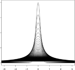
To elucidate the challenges of this type of modeling problem, we begin with a simple example. Imagine our dictionary consists of $\mu=0$ Gaussian functions generated over a fine grid of $\sigma$, such as those in Figure 1. We observe a set of objects, each producing data from a different function constructed as a sparse linear combination of the dictionary of Gaussian functions. The data from each object are sampled across a fixed grid with additive i.i.d. Gaussian noise. The component weights are constrained to be nonnegative and sum to 1, ensuring that all parameters are physically-plausible (e.g., $\bar{\sigma}>0$).

Figure 1: Database of Gaussian curves used in the example in Section 1.1. Simulated data are generated as noisy random sparse linear combinations of these curves. As $\sigma$ increases, it becomes more difficult to distinguish the curves, especially in the presence of noise. A basis of prototypes for estimation of the target parameter, $\bar{\sigma}$, should include a higher proportion of low-$\sigma$ Gaussian curves.

Our ultimate goal is to estimate a set of target parameters for each observed data point. In this example, our target is $\bar{\sigma}$, the weighted average $\sigma$ of the component Gaussian curves of each observed data vector. To this end, we model each observed curve as a linear superposition of a set of prototypes and use the estimated prototype weights to estimate $\bar{\sigma}$.

If our goal were to reconstruct each data point with as small of error as possible, then a prototyping approach that samples along the boundary of the convex hull of the dictionary of Gaussian functions (such as archetypal analysis, see Section 4.2.1) would be optimal. In this paper, the goal is to achieve small errors in the target parameter estimates. A common approach for this problem is to sample prototypes uniformly over the parameter space. However, this often leads to the inclusion of many prototypes with nearly identical curves. Consider the Gaussian curve example: for high values of $\sigma$, the curves do not change considerably with respect to changes in $\sigma$. Under the presence of noise, curves with large $\sigma$ are not distinguishable. We are better off including a higher proportion of prototypes in the low-$\sigma$ range, where curves change more with respect to changes in $\sigma$.

This intuition leads us to a different approach: choose prototypes by quantizing the space of curves (see Section 4.1). We show in Section 5.1 that a method that selects prototypes by quantizing the vector space of theoretical components outperforms the method of choosing prototypes from a uniform grid of $\sigma$ in the estimation of $\bar{\sigma}$ (see Figure 5). Additionally, judicious selection of a reduced prototype basis is an effective regularization of an estimation problem that is subject to large variance when the full range of theoretical components are utilized without any smoothing. The simulation results shown below will display markedly reduced variances in the estimates of the parameters of interest relative to the same procedures using larger libraries of basis functions.

Additionally, smaller prototype bases yield better parameter estimates than the approach of using all of the theoretical components to model observed data, a phenomenon that can be explained by the markedly reduced variance of parameter estimates found by smaller, judiciously-chosen bases.

1.2 Paper organization

The paper is organized as follows. In Section 2 we detail the problem of estimating star formation history parameters for galaxies and explain how prototyping methods can be used to obtain accurate parameter estimates. In Section 3 we formalize the problem of prototype selection for target parameter estimation and in Section 4 describe several approaches. We apply those methods to simulated data in Section 5 to compare their performances. In Section 6 we return to the astrophysics example, applying our methods to galaxy data from the Sloan Digital Sky Survey. We end with some concluding remarks in Section 7.

2 Modeling galaxy star formation history

Galaxies are gravitationally-bound objects containing $10^{5}$–$10^{10}$ stars, gas, dust and dark matter. The characteristics of the light we detect from each galaxy primarily depend on the physical parameters (e.g., age and composition) of its component stars as well as distortions due to dust that resides in our line of sight to that galaxy, spectral distortions due to the line-of-sight component of the orbital velocities of its component stars, and the distance to the galaxy.

The physical mechanisms that govern galaxy formation and evolution are complicated and poorly understood. Galaxies are complex, dynamic objects. The star formation rate (SFR) of each galaxy tends to change considerably throughout its lifetime and the patterns of SFR vary greatly between different galaxies. The SFR for each galaxy depends on a countless number of factors, such as merger history, the galaxy’s local environment (e.g., the matter density of its neighborhood, and the properties of surrounding galaxies) and chemical composition. Astronomers are interested in refining galaxy evolution models so that they match the observed patterns of galaxy SFH in the Universe. It is imperative that we first have accurate estimates of the star formation history parameters for each observed galaxy. These SFH estimates are necessary to test competing physical models, alert to possible shortcomings in current models, and estimate cosmological parameters [for an example of such an analysis, see Asari et al. (2007)].

2.1 Population synthesis model

A common technique in the astronomy literature, called empirical population synthesis, is to model each galaxy as a mixture of stars from different simple stellar populations (SSPs), defined as groups of stars with the same age and metallicity ($Z$, defined as the fraction of mass contributed by any element heavier than helium). The principle behind this method is that each galaxy consists of multiple subpopulations of stars of different age and composition so that the integrated observed light from each galaxy is a mixture of the light contributed by each SSP. Describing the data from each galaxy as a combination of SSPs allows us to reconstruct the star formation and metallicity history of each galaxy. This is because, for each galaxy, the component weight on an SSP captures the proportion of that galaxy’s stars that was created at the specific epoch corresponding to the age of that SSP. Therefore, the full vector of SSP component weights for each galaxy describes the star formation throughout the galaxy’s lifetime.

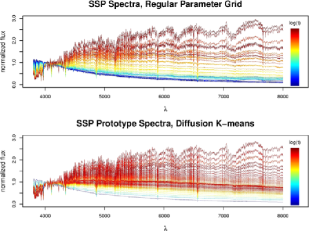
Theoretical SSPs can be produced by physical models, that are in turn constrained by observational studies. These models typically start with a set of initial conditions and evolve the system forward in time based on sets of physically motivated differential equations. The output produced by these models can be extremely detailed. In our study, we use a set of high-resolution, broad-band spectra from the SSP models of Bruzual and Charlot (2003). See Figure 2 for an example of some SSP spectra, plotted over the optical portion of the electromagnetic spectrum.

Figure 2: Two bases of SSP spectra of size $K=45$, colored by $\log t$. Each spectrum is normalized to 1 at $\lambda_{0}=4020$ Å. Top: basis of regular ($t,Z$) grid used in Cid Fernandes et al. (2005). Bottom: diffusion $K$-means basis used in Richards et al. (2009a). The diffusion $K$-means basis shows a more gradual sampling of spectral space than the regular grid basis, which over-samples spectra from young stellar populations.

The galaxy data we use to estimate SFH parameters are high-resolution, broad-band spectra from the Sloan Digital Sky Survey [SDSS, York et al. (2000)] which consist of light flux measurements over thousands of wavelength bins. To model the data from each galaxy, we adopt the empirical population synthesis generative model of a galaxy spectrum introduced in Cid Fernandes et al. (2004):

$$\qquad{\mathbf{Y}}_{\lambda}(\bolds{\gamma},M_{\lambda_{0}},A_{V},v_{*},\sigma_{*})=M_{\lambda_{0}}\Biggl{(}\sum_{j=1}^{N}\gamma_{j}{\mathbf{X}}_{j,\lambda}r_{\lambda}(A_{V})\Biggr{)}\otimes G(v_{*},\sigma_{*}),$$ (1)

where ${\mathbf{Y}}_{\lambda}$ is the light flux at wavelength $\lambda$. The components of model (1) are the following:

• ${\mathbf{X}}_{j}$ is the $j$th SSP spectrum normalized at wavelength $\lambda_{0}$. Each SSP has age $t({\mathbf{X}}_{j})$ and metallicity $Z({\mathbf{X}}_{j})$. In the true generative model, ${\mathbf{X}}$ contains an infinite number of SSP spectra over the continuous parameters of age and metallicity.

• $\gamma_{j}\in[0,1]$, the component proportion of the $j$th SSP. The vector $\gamma$ is the population vector of the galaxy, the principal parameter of interest for calculating derived parameters describing the SFH of a galaxy.

• $M_{\lambda_{0}}$, the observed flux at wavelength $\lambda_{0}$.

• $r_{\lambda}(A_{V})$ accounts for the wavelength-dependent fraction of light that is either absorbed or scattered out of the line of sight by foreground dust. $A_{V}$ parametrizes the amount of this dust extinction that occurs. We adopt the reddening model of Cardelli, Clayton and Mathis (1989).

• Convolution, in wavelength, by the Gaussian kernel $G(v_{*},\sigma_{*})$ describes spectral distortions from Doppler shifts caused by the movement of stars within the observed galaxy with respect to our line-of-sight, and is parametrized by a central velocity $v_{*}$ and dispersion $\sigma_{*}$. Previous to the analysis, care was taken to properly resample all spectra—both the observed and model spectra—to 1 measurement per Ångström. This was done to ensure the reliability of the spectral errors when used by the STARLIGHT spectral fitting software. More details are available at http://www.starlight. ufsc.br/papers/Manual_StCv04.pdf.

2.2 SSP basis selection and SFH parameter estimation

For each galaxy, we observe a flux, $\mathbf{O}_{\lambda}$, at each spectral wavelength, $\lambda$, with corresponding standard error, $\widehat{\sigma}_{\lambda}$, estimated from photon counting statistics and characteristics of the telescope and detector. To estimate the target SFH parameters for each galaxy, we use the STARLIGHT software of Cid Fernandes et al. (2005), fitting model (1) using maximum likelihood. The code uses a Metropolis algorithm with simulated annealing to minimize

$$\chi^{2}(\bolds{\gamma},M_{\lambda_{0}},A_{V},v_{*},\sigma_{*})=\sum_{\lambda=1}^{N_{\lambda}}\biggl{(}\frac{\mathbf{O}_{\lambda}-{\mathbf{Y}}_{\lambda}}{\widehat{\sigma}_{\lambda}}\biggr{)}^{2},$$ (2)

where ${\mathbf{Y}}_{\lambda}$ is the model flux in (1). The optimization routine searches for the maximum likelihood solution for the model $\mathbf{O}_{\lambda}\sim N({\mathbf{Y}}_{\lambda},\widehat{\sigma}_{\lambda})$, i.i.d. for each $\lambda$. The minimization of (2) is performed over $N+4$ parameters: $\gamma_{1},\ldots,\gamma_{N},M_{\lambda_{0}},A_{V}$, $v_{*}$, and $\sigma_{*}$. The speed of the algorithm scales as $\mathcal{O}(N^{2})$, so it is imperative to pick a SSP basis with a small number of spectra.

In practice, we use a basis of $K\ll N$ prototype SSP spectra, $\bolds{\Psi}=\{\bolds{\Psi}_{1},\ldots,\allowbreak\bolds{\Psi}_{K}\}$—which can be a carefully chosen subset or a nontrivial combination of the ${\mathbf{X}}_{j}$’s—and model each galaxy spectrum as

$$\qquad{\mathbf{Y}}_{\lambda}(\bolds{\beta},M_{\lambda_{0}},A_{V},v_{*},\sigma_{*})=M_{\lambda_{0}}\Biggl{(}\sum_{k=1}^{K}\beta_{k}\bolds{\Psi}_{k,\lambda}r_{\lambda}(A_{V})\Biggr{)}\otimes G(v_{*},\sigma_{*}),$$ (3)

where each prototype, $\bolds{\Psi}_{j}$, has age $t(\bolds{\Psi}_{k})$ and metallicity $Z(\bolds{\Psi}_{k})$, and$\sum_{k=1}^{K}\beta_{k}=1$.

Our goal in this analysis is to choose a suitable SSP basis to estimate a set of physical parameters for each galaxy. Some of the commonly-used SFH parameters are as follows:

• $\langle\log t\rangle_{L}=\sum_{i=1}^{N}\gamma_{i}\log t({\mathbf{X}}_{i})$, the luminosity-weighted average log age of the stars in the galaxy,

• $\log\langle Z\rangle_{L}=\log\sum_{i=1}^{N}\gamma_{i}Z({\mathbf{X}}_{i})$, the log luminosity-weighted average metallicity of the stars in the galaxy,

• $\gamma_{c}$, a time-binned version of the population vector, $\gamma$, and

• $\langle\log t\rangle_{M},\log\langle Z\rangle_{M}$, mass-weighted versions of the average age and metallicity of the stars in the galaxy.

We estimate each of these parameters using the maximum likelihood parameters from model (3). In Richards et al. (2009a), we introduced a method of choosing a SSP prototype basis and compared it to bases of regular $(t,Z)$ grids that were used in previous analyses. See Figure 2 for a plot of two such SSP spectral bases.

3 Formal problem statement

We begin with a large, fixed set of $N$ theoretical components, each with known parameters $\bolds{\pi}_{i}$ (these are the physical properties of each component). We refer to this set as the model data. These data can be thought of as a sample from some distribution $P_{X}$ in $\mathbb{R}^{p}$. The model data are stored in an $p$ by $N$ matrix ${\mathbf{X}}=[{\mathbf{X}}_{1},\ldots,{\mathbf{X}}_{N}]$, where $p$ is the total wavelength range of the SSP spectra. We assume that each observed data point ${\mathbf{Y}}_{j}$, $j=1,\ldots,M$, is generated from the linearly separable nonlinear model

$${\mathbf{Y}}_{j}=f\Biggl{(}\sum_{i=1}^{N}\gamma_{ij}{\mathbf{X}}_{i};\bolds{\theta}_{j}\Biggr{)}+\bolds{\varepsilon}_{j},$$ (4)

where, for each $j$, the coefficients, $\gamma_{1j},\ldots,\gamma_{Nj}$, are nonnegative and sum to 1. The functional $f$ is a known, problem-dependent (possibly nonlinear) function of the linear combination of the components ${\mathbf{X}}$ and some unknown parameters, $\theta_{j}$. Each $\bolds{\varepsilon}_{j}$ is a vector of random errors. The set of target parameters for each observed data vector, ${\mathbf{Y}}_{j}$, is $\{\rho_{j},\theta_{i}\}$, where $\rho_{j}=\sum_{i=1}^{N}\gamma_{ij}\pi_{i}$ is a function of the model weights, $\gamma$, and intrinsic parameters, $\pi$, of the theoretical components.

For large $N$, it is impossible to use model (4) to estimate each $\{\rho_{j},\theta_{j}\}$ due to the large computational cost. Our goal is to find a set of prototypes $\bolds{\Psi}=[\bolds{\Psi}_{1},\ldots,\bolds{\Psi}_{K}]$, where $K\ll N$, that can accurately estimate the target parameters $\{\rho_{j},\theta_{j}\}$ for each observed ${\mathbf{Y}}_{j}$, using the model

$${\mathbf{Y}}_{j}=f\Biggl{(}\sum_{k=1}^{K}\beta_{kj}\bolds{\Psi}_{k};\bolds{\theta}_{j}\Biggr{)},$$ (5)

where $\beta_{1j},\ldots,\beta_{Kj}$ are nonnegative component weights such that $\sum_{k}\beta_{kj}=1$ for all $j$. Naturally, our estimate of $\rho_{j}$ is

$$\widehat{\rho}_{j}=\sum_{k=1}^{K}\widehat{\beta}_{kj}\sum_{i=1}^{N}\alpha_{ik}\pi_{i},$$ (6)

where the $\widehat{\beta}_{jk}$ are estimated using the model (5), and $\bolds{\alpha}$ is an $N$ by $K$ matrix of nonnegative coefficients that defines the prototypes from the dictionary of components by

$$\bolds{\Psi}={\mathbf{X}}\bolds{\alpha}.$$ (7)

The coefficients $\bolds{\alpha}$ are constrained such that each of the prototypes, $\bolds{\Psi}_{k}$, resides in a region of the theoretical component space, $R_{k}\in\mathcal{X}$, with nonzero probability, $P_{X}(R_{k})>0$, over all plausible values of the physical parameters used to generate ${\mathbf{X}}$. This constraint is enforced to ensure the physical plausibility of the prototypes, $\bolds{\Psi}$, and their parameters. If our prototype basis were to include components that are disallowed by the physical models that generated ${\mathbf{X}}$, then the parameter estimates for the observed data would be uninterpretable.

4 Methods for prototyping

The usual method used to choose a basis for estimating target parameters from the signal model is to select prototypes from a regular grid in the physical parameter space. Examples of such bases are those found in Cid Fernandes et al. (2005) and Asari et al. (2007), both of whom employ SSPs on regular grids of age and metallicity to estimate SFH parameters. In this section we propose methods that use the set of physical components, ${\mathbf{X}}$, to construct a prototype basis in a principled manner. In Section 5 we compare the proposed basis selection methods via simulations, and show that regular parameter grids tend to yield suboptimal parameter estimates.

4.1 Quantization of model space

For problems of interest, practical fitting of theoretical models to noisy data requires a finite set of prototypes. The question becomes how to best choose this set of prototypes, that is, how to quantize the model space. Here, instead of quantizing the parameter space by choosing uniform parameter grids, we propose methods that quantize the vector space $\mathcal{X}$ of theoretical model-produced data. The idea behind this approach is that under the presence of noise, components with similar functional forms will be indistinguishable, so that it is better to choose prototypes that are approximately evenly spaced in $\mathcal{X}$ (rather than evenly spaced in the parameter space). By replacing the theoretical models in each neighborhood by their local average, the model quantization approach is optimal for treating degeneracies because it allows a slight increase in bias to achieve a large decrease in variance of the target parameter estimates. The increase in estimator bias should be small because more prototypes are included in parameter regions where we can better discern the theoretical data curves of the components, allowing for precise parameter estimates in those regions and coarser average estimates in degenerate regions. If, instead, multiple components in our dictionary were to have very similar theoretical data curves but different parameter values, then, in the absence of any other method of regularization, we would have difficulty breaking the degeneracy no matter how many prototypes we include in that region of the parameter space, causing increased parameter estimator variance and higher statistical risk.

4.1.1 $K$-means and diffusion $K$-means

The basic idea here is to quantize the vector space or support of model-produced data with respect to an appropriate metric and prior distribution. The vector quantization approach can be formalized as follows:

Suppose that $\mathbf{X}_{1},\ldots,\mathbf{X}_{N}$ is a sample from some distribution $P_{X}$ with support $\mathcal{X}\subset\mathbb{R}^{p}$. The support $\mathcal{X}$ often has some lower-dimensional structure, which we refer to as the lower-dimensional geometry of $\mathcal{X}$. Fix an integer $K<N$. To any dictionary $A=\{\mathbf{a}_{1},\ldots,\mathbf{a}_{K}\}$ of prototypes, we can assign a cost

$$W(A,P_{X})=\int{\min_{\mathbf{a}\in A}}\|\mathbf{x}-\mathbf{a}\|^{2}P_{X}(d\mathbf{x}).$$ (8)

Let $\mathcal{B}_{k}$ denote all sets of the form $B=\{\mathbf{b}_{1},\ldots,\mathbf{b}_{K}\}$ with $\mathbf{b}_{j}\in\mathbb{R}^{p}$. Define the optimal dictionary of $K$ prototypes as the cluster centers

$$\bolds{\Psi}=\mathop{\arg\min}_{B\in\mathcal{B}_{k}}W(B,P_{X}).$$

In practice, we estimate $\bolds{\Psi}$ from model-produced data $\mathbf{X}_{1},\ldots,\mathbf{X}_{N}$ according to

$$\widehat{\bolds{\Psi}}=\mathop{\arg\min}_{B}W(B,\widehat{P}_{X}),$$

where $\widehat{P}_{X}$ is the empirical distribution. This estimate is found by Lloyd’s $K$-means (KM) algorithm. To simplify the notation, we will henceforth skip the hat symbol on all estimates.

The empirical $K$-means solution corresponds to allocating each $\mathbf{X}_{i}$ into subsets $S_{1},\ldots,S_{K}$, where the $K$ centroids define the prototypes. In the definition of the prototypes in (7), this reduces to

$$\alpha_{ik}=\cases{\dfrac{1}{|S_{k}|},&\quad if $i\in S_{k}$,\vspace*{2pt}\cr 0,&\quad else.}$$ (9)

Potential problems to this approach are the following: (1) the KM prototypes will adhere to the design density on $\mathcal{X}$, and (2) for small $K$, estimated prototypes could fall in areas that $P_{X}$ assigns probability zero. The first issue can be corrected using a weighted $K$-means approach or a method such as uniform subset selection (Section 4.1.2). However, often the density on $\mathcal{X}$ corresponds to a prior distribution on the physical parameters, meaning it is often desirable to adhere to its design density. To remedy the latter issue, we could select as prototypes the $K$ data points that are closest to each of the centroids. We see in simulations that this approach tends to yield slightly worse parameter estimates than the original $K$-means formulation. We attribute this to the smoother sampling of parameter space achieved by the original KM formulation, which averages the parameters of components with similar theoretical data, effectively decreasing the variability of the parameter estimates.

If the theoretical data are high dimensional, we might choose to first learn the low-dimensional structure of ${\mathbf{X}}$ and then employ $K$-means in this reduced space. This would permit us to avoid quantizing high-dimensional data, where $K$-means can be problematic due to the curse of dimensionality. This failure occurs because the theoretical data are extremely sparse in high dimensions, causing the distances between similar components to approach the distances between unrelated objects. To remedy this, we suggest the use of the diffusion map method for nonlinear dimensionality reduction [Coifman and Lafon (2006), Lafon and Lee (2006)]. In other words, we transform the model data into a lower-dimensional representation where we apply $K$-means (diffusion $K$-means, DKM). Formally, this corresponds to substituting (8) with the cost function

$$W(\phi,A,P_{X})=\int{\min_{\mathbf{a}\in A}}\|\phi(\mathbf{x})-\phi(\mathbf{a})\|^{2}P_{X}(d\mathbf{x}),$$ (10)

where $\phi$ is a data transformation defined by diffusion maps.

4.1.2 Uniform subset selection

In the theoretical model data quantization approach the goal is to have prototypes regularly spaced in $\mathcal{X}$, where $\mathcal{X}$ is the support of $P_{X}$. With this heuristic in mind, we devise the uniform subset selection (USS) method, which sequentially chooses the component ${\mathbf{X}}_{i}\in{\mathbf{X}}$ that is furthest away from the closest component that has already been chosen. Because the choice of distance metric is flexible, USS can be tailored to deal with many data types and high-dimensional data. Unlike $K$-means, USS is not influenced by differences in the density of components across $\mathcal{X}$. However, USS typically chooses extreme components as prototypes because in each successive selection it picks the furthest theoretical data curve from the active set. In simulations, USS produces poor parameter estimates due to its tendency to select extreme components.

4.2 Sparse coding approaches

Most standard sparse coding techniques do not apply for the prototyping problem. Without the appropriate constraints, the prototype basis elements will be nonphysical and the subsequent parameter estimates will be nonsensical (see Section 4.2.3). There are methods related to sparse coding that enforce the proper constraints to ensure that prototype basis elements reside within the native data space (see Sections 4.2.1 and 4.2.2), but these generally do not perform well for target parameter estimation because their objective of optimal data reconstruction—and not estimation of the target parameters—forces these methods to choose extreme prototypes.

4.2.1 Archetypal analysis

Archetypal analysis (AA) was introduced by Cutler and Breiman (1994) as a method of representing each data point as a linear mixture of archetypal examples, which themselves are linear mixtures of the original component dictionary. The method searches for the set of archetypes $\bolds{\Psi}_{1},\ldots,\bolds{\Psi}_{K}$ that satisfy (7) and minimize the residual sum of squares (RSS)

$$\mathrm{RSS} = \sum_{i=1}^{N}\Biggl{\|}{\mathbf{X}}_{i}-\sum_{k=1}^{K}\beta_{ik}\bolds{\Psi}_{k}\Biggr{\|}^{2}$$ (11)

$$= \sum_{i=1}^{N}\Biggl{\|}{\mathbf{X}}_{i}-\sum_{k=1}^{K}\beta_{ik}\sum_{j=1}^{N}\alpha_{jk}{\mathbf{X}}_{j}\Biggr{\|}^{2},$$ (12)

where $\sum_{k=1}^{K}\beta_{ik}=1$ for all $i$ and $\beta_{ik}\geq 0$ for all $i$ and $k$. To minimize the RSS criterion, an alternating nonnegative least squares algorithm is employed, alternating between finding the best $\bolds{\beta}$’s for a set of prototypes and finding the best prototypes ($\bolds{\alpha}$’s) for a set of $\bolds{\beta}$’s. This computation scales linearly in the number of dimensions of the original theoretical data, with computational complexity becoming prohibitive for dimensionality more than 500 [Stone (2002)].

Once there are as many prototypes, $K$, as the number of data points that define the boundary of the convex hull, any element in the dictionary can be fit perfectly with a linear mixture of the prototypes, yielding a RSS of 0. If we try to pick more prototypes than the number of data points that define the boundary of the convex hull, then the AA algorithm will fail to converge because $\beta$ becomes noninvertible, preventing the iterative algorithm to find the optimal set of prototypes, $\bolds{\Psi}=\beta^{-1}{\mathbf{X}}$, given the current $\beta$. We have experimented with using the Moore–Penrose pseudoinverse to perform this operation, but it is usually ill-behaved when $\beta$ is noninvertible. This upper bound on the number of AA prototypes is a serious drawback to using AA as a prototyping method because often the complicated nature of the data generating processes necessitates the use of larger prototype bases.

Prototypes found by AA are optimal in the sense that they minimize the RSS for fitting noiseless, linear mixtures of the ${\mathbf{X}}$’s. This is the case because AA prototypes are found along the boundary of the convex hull formed by the ${\mathbf{X}}$’s [see Cutler and Breiman (1994)]. Unlike AA, our objective is not to minimize RSS, but to minimize the error in the derived parameter estimates. Archetypal analysis achieves suboptimal results in the estimation of $\bolds{\rho}$ because it only samples prototypes from the boundary of the component space, $\mathcal{X}$, focusing attention on extreme cases while disregarding large regions of $\mathcal{X}$. In Section 5 we show using simulated data that AA is outperformed by the model quantization approach for estimating the target parameters from the signal model parameters.

4.2.2 Sparse subset selection

We introduce the method of sparse subset selection (SSS), whose goal is to find a subset of the original dictionary, $\bolds{\Psi}\subset{\mathbf{X}}$, that can reconstruct ${\mathbf{X}}$ in a linear mixture setting. This method is motivated by sparse coding in that it seeks the basis that minimizes a regularized reconstruction of ${\mathbf{X}}$, where the regularization is chosen to select a subset of the columns of ${\mathbf{X}}$.

Recently, Obozinski et al. (2011) introduced a method of variable selection in a high-dimensional multivariate linear regression setting. Their method uses a penalty on the $\ell_{1}/\ell_{q}$ norm, for $q>1$, of the matrix of regression coefficients in such a way that induces sparsity in the rows of the coefficient matrix. We can, in a straightforward way, adapt their method to select a subset of columns of ${\mathbf{X}}$ to be used as prototypes. Our objective function is

$$\mathop{\arg\min}_{{\mathbf{B}}}\biggl{\{}\frac{1}{2N}\|{\mathbf{X}}-{\mathbf{X}}{\mathbf{B}}\|_{F}^{2}+\lambda_{k}\|{\mathbf{B}}\|_{\ell_{1}/\ell_{q}}\biggr{\}},$$ (13)

where $\|\cdot\|_{F}$ is the Frobenius norm of a matrix, and the $\ell_{1}/\ell_{q}$ penalty is defined as

$$\|{\mathbf{B}}\|_{\ell_{1}/\ell_{q}}=\sum_{i=1}^{N}\Biggl{(}\sum_{j=1}^{N}b_{ij}^{q}\Biggr{)}^{1/q}=\sum_{i=1}^{N}\|b_{i}\|_{q}$$ (14)

so that sparsity is induced in the rows of ${\mathbf{B}}$, the $N$ by $N$ matrix of nonnegative mixture coefficients. Additionally, ${\mathbf{B}}$ is normalized to sum to 1 across columns. The basis, $\bolds{\Psi}$, is defined as the columns of ${\mathbf{X}}$ that correspond to nonzero rows of ${\mathbf{B}}$ ($\bolds{\alpha}$ is the corresponding indicator variable). The parameter $\lambda_{k}$ controls the number of prototypes in our SSS set $\bolds{\Psi}$.

To perform the optimization (13), we use the CVX Matlab package [Grant and Boyd (2010)]. Setting $q=2$, we recast the problem as a second-order cone problem with the additional constraints of nonnegativity and column normalization of ${\mathbf{B}}$ [see Boyd and Vandenberghe (2004)]. The current implementation cannot solve problems for large $N$. In Section 4.3 we show, for a small problem, that SSS has behavior similar to archetypal analysis in that it selects prototypes from the boundary of the convex hull of ${\mathbf{X}}$. Like AA, SSS is not a good method for target parameter estimation.

4.2.3 Some methods not useful for prototyping

There are other methods for sparse data representation that fail to work for prototype selection. These methods are not applicable to this problem because they do not select prototypes that reside in regions of $\mathcal{X}$ with nonzero probability $P_{X}$. The failure to obey this constraint means that the chosen prototypes in general will not be physical, meaning that either their theoretical data or intrinsic parameters are disallowed. For instance, in the SFH problem, this could lead us to use prototypes whose spectra have negative photon fluxes or whose ages are either negative or greater than the age of the Universe. Using such uninterpretable prototypes to model observed data produces parameter estimates that are nonsensical.

We mention two popular methods for estimating small bases from large dictionaries, ${\mathbf{X}}$, and describe why they are not useful for prototyping:

In standard sparse coding [Olshausen et al. (1996)], the goal is to find a decomposition of the matrix ${\mathbf{X}}$, in which the hidden components are sparse. Sparse coding combines the goal of small reconstruction error along with sparseness, via minimization of

$$C(\bolds{\Psi},{\mathbf{A}})=\frac{1}{2}\|{\mathbf{X}}-\bolds{\Psi}{\mathbf{A}}\|^{2}+\lambda\sum_{ij}|a_{ij}|,$$ (15)

where the trade-off between $\ell_{1}$ sparsity in the mixture coefficients ${\mathbf{A}}$, and accurate reconstruction of ${\mathbf{X}}$, is controlled by $\lambda$. However, there are no constraints on the sign of the entries of ${\mathbf{A}}$ or $\bolds{\Psi}$, meaning that prototypes with nonphysical attributes are allowed.

Nonnegative Matrix Factorization (NMF) [Lee and Seung (2001), Paatero and Tapper (1994)] is a related technique that includes strict nonnegativity constraints on all coefficients $a_{ij}$ and $\Psi_{jk}$ while minimizing the reconstruction of ${\mathbf{X}}$,

$$\mathop{\arg\min}_{\Psi,{\mathbf{A}}}\biggl{\{}\frac{1}{2}\|{\mathbf{X}}-\bolds{\Psi}{\mathbf{A}}\|^{2}\biggr{\}}.$$ (16)

This construction is different than our prototype definition in (7), where $\bolds{\Psi}={\mathbf{X}}\bolds{\alpha}$. To reconcile the two, we see that, since $N>K$, $\bolds{\alpha}$ is the right inverse of ${\mathbf{A}}$:

$$\bolds{\alpha}={\mathbf{A}}({\mathbf{A}}^{T}{\mathbf{A}})^{-1},$$ (17)

which exists if ${\mathbf{A}}$ is full rank. However, under this formulation, the $\alpha_{ij}$ are not constrained to be nonnegative and the resultant prototypes are not constrained to reside in $\mathcal{X}$. Thus, NMF is not useful for prototyping. Note that archetypal analysis avoids this problem by enforcing the further constraint that the prototypes be constrained linear combinations of ${\mathbf{X}}$.

4.3 Comparison of prototypes

We apply four prototyping methods to the two-dimensional data set toy in the archetypes R package. We treat each 2-D data point, ${\mathbf{X}}_{i}$, as model-produced theoretical data. Plots of this dictionary of data and the selected prototypes for four different prototyping methods, using $K=7$, are in Figure 3. $K$-means places prototypes evenly spaced within the convex hull of the data. USS also evenly allocates the prototypes, but

Figure 3: Distribution of prototypes (red $\blacktriangle$’s) for four different methods when applied to the 250 theoretical data objects in the toy data set (grey $\bullet$’s). $K$-means evenly samples the native data space while the other methods focus more attention to the boundary of the space.

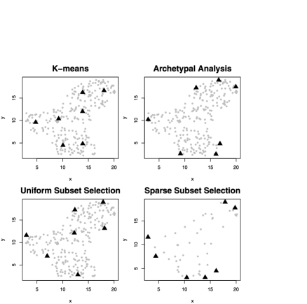
places many along the boundary of the native space. Archetypal analysis and SSS place all prototypes on the boundary of the convex hull. Note that for more than 7 prototypes, the archetypal analysis algorithm does not converge to a solution.

5 Simulated examples

In this section we test the effectiveness of the prototyping methods for estimating a set of target parameters using simulated data. The first test set is the toy example of zero-mean Gaussian curves discussed in Section 1.1. The second simulation experiment is a set of realistic galaxy spectra created to mimic the SDSS data that we later analyze in Section 6.

5.1 Gaussian curves

We begin with the example introduced in Section 1.1. We simulate a database of $N=157,\mu=0$ Gaussian curves, ${\mathbf{X}}_{1},\ldots,\allowbreak{\mathbf{X}}_{N}$, on a fine grid of $\sigma=(\sigma_{1},\ldots,\sigma_{N})$ from 0.2 to 8 in steps of 0.05 (see Figure 1). Each ${\mathbf{X}}_{i}$ is represented as a vector of length 321. From this database, we simulate a set of 100 data vectors, ${\mathbf{Y}}_{1},\ldots,{\mathbf{Y}}_{100}$, from the model

$${\mathbf{Y}}_{j}=\sum_{i=1}^{N}\gamma_{ij}{\mathbf{X}}_{i}+\varepsilon_{j},$$ (18)

where the mixture coefficients, $\gamma_{ij}\geq 0$, sum to unity for each $j$ and have at most 5 nonzero entries for each $j$. The noise vectors, $\varepsilon_{j}$, are i.i.d. normal zero-mean with standard deviation 0.05.

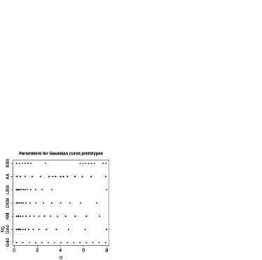
From ${\mathbf{X}}_{1},\ldots,{\mathbf{X}}_{N}$, we generate bases of prototypes using six different methods described in Section 4. To explore the differences in each of these methods, we plot (Figure 4) the distribution of $K=15$ prototype $\sigma$ values. The model quantization methods (KM, DKM, USS) find more prototypes with small $\sigma$ values. The AA and SSS methods place more prototypes at the extreme values of $\sigma$ (note that for SSS, we ran the algorithm on a coarser grid of 32 Gaussian curves).

Figure 4: Distribution of $K=15$ prototype $\sigma$ values for seven different prototyping methods applied to the Gaussian curves example. The methods are the following: Grid-regular $\sigma$ grid, log Grid-regular $\log(\sigma)$ grid, KM—$K$-means, DKM—diffusion $K$-means, USS—uniform subset selection, AA—archetypal analysis, and SSS—sparse subset selection.

To evaluate each of the methods, we compare their ability to estimate the average $\sigma$ for each ${\mathbf{Y}}_{j}$, defined as

$$\bar{\sigma}_{j}=\sum_{i=1}^{N}\gamma_{ij}\sigma_{i}.$$ (19)

For each choice of basis, we fit the observed data using nonnegative least squares. In Figure 5 the MSE for $\bar{\sigma}$ estimation for $K$-means, diffusion $K$-means, USS and uniform $\sigma$-grid and $\log(\sigma)$ grid bases is plotted as a function of $K$. SSS is not plotted because it yields parameter estimates with MSE $>2$. AA is not plotted because it only converges for $K\leq 15$, and performs worse than the $\sigma$ grid for those values. KM and DKM outperform the regular parameter grids, USS, and AA prototype bases. KM achieves a minimum MSE, averaged over 25 trials, of 0.815 at $K=10$ prototypes. DKM achieves a minimum MSE of 0.846 at $K=15$ prototypes, while the uniform $\sigma$ grid achieves a minimum MSE of 1.378, 1.7 times higher than the best MSE for KM. Results for AA and SSS are not plotted because AA only converges for $K\leq 15$ prototypes, and SSS is too computationally intensive to run on the entire dictionary of curves; at $K=15$, neither method outperforms a uniform $\sigma$ grid.

Figure 5: MSE for the estimation of $\sigma$ for the Gaussian curve example. Plotted is the MSE for using a regular parameter grid, $K$-means (KM), diffusion $K$-means (DKM) and archetypal analysis (AA) prototype bases. Both DKM and KM achieve significantly better $\bar{\sigma}$ estimates than a regular parameter grid and outperform estimates obtained by using all 157 Gaussian curves in the original dictionary. For each $K$, the MSE is averaged across 25 repetitions of the experiment. Point-wise 68% confidence bands are shown as dotted lines.

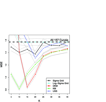
An interesting observation in Figure 5 is that the minimum MSE for estimating ${\bar{\sigma}}$ is achieved for $K=10$ KM prototypes. As the number of prototypes increases from 10, the KM $\bar{\sigma}$ estimates worsen. This exemplifies the bias-variance trade-off in the estimation procedure: for $K>10$, the increased variance of the estimates is larger than the reduction in squared-bias. Estimates of $\bar{\sigma}$ from four of the five prototype bases plotted in Figure 5 outperform the estimates found by fitting each ${\mathbf{Y}}_{j}$ as a mixture of all 157 original component curves. Over the 25 repetitions of the simulations, the $\gamma_{ij}$ which are positive, that is, the $\mathbf{X}_{i}$ that receive any weight, vary widely. These results demonstrate that a single, judiciously chosen, reduced basis can reproduce a wide range of truths and return accurate parameter estimates with reduced variance.

5.2 Simulated galaxy spectra

We further test the performance of each prototyping method using realistic simulated galaxy spectra. Starting with a database, ${\mathbf{X}}$, of 1,182 SSPs from the models of Bruzual and Charlot (2003) (see Section 2), we generate simulated galaxy spectra using the model (1). The SSPs are generated from 6 different metallicities and a fine sampling of 197 ages from 0 to 14 Gyrs. We use a prescription similar to Chen et al. (2009) to choose the physical parameters of the simulations, altered to have higher contribution from younger SSPs. The basic physical components of the simulation are as follows: [(1)]

A star formation history with exponentially decaying star formation rate (SFR): SFR $\propto\exp(\gamma t)$. Here, $\gamma>0$, so the SFR is exponentially declining with time, as $t$ is the age of the SSP today.

We allow $\gamma$ to vary between galaxies. For each galaxy we draw $\gamma$ from a uniform distribution between 0.25 and 1 $\mathrm{Gyr}^{-1}$.

The time $t_{\mathrm{form}}$ when a galaxy begins star formation is distributed uniformly between 0 and 5.7 Gyr after the Big Bang, where the Universe is assumed to be 13.7 Gyr old.

We allow for starbursts, epochs of increased SFR, with equal probability at all times. The probability a starburst begins at time $t$ is constructed so that the probability of no starbursts in the life of the galaxy is 33%. The length of each burst is distributed uniformly between 0.03 and 0.3 Gyr and the fraction of total stellar mass formed in the burst in the past 0.5 Gyr is distributed log-uniformly between 0 and 0.5. The SFR of each starburst is constant throughout the length of the burst. Each galaxy spectrum is generated as a mixture of SSPs of up to 197 time bins, with a uniformly drawn metallicity in each bin. We draw the reddening parameter ($A_{V}$) and velocity dispersion ($\sigma_{0}$) from empirical distributions over a plausible range of each parameter. We simulate 100 galaxy spectra with i.i.d. zero-mean Gaussian noise with $\mbox{S}/\mbox{N}=10$ at $\lambda_{0}=4020$ Å.

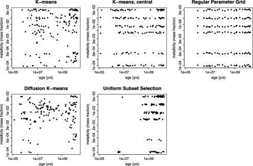
We apply the methods in Section 4 to choose SSP prototype bases from ${\mathbf{X}}$. In Figure 6 the distributions of the SSP prototype ages and metallicities for $K=150$ prototype bases are plotted along with the regular parameter grid used by Asari et al. (2007). Each method highly samples the older, higher metallicity SSPs and typically only includes a few prototypes with low age and low metallicity. This is reasonable because older, higher metallic SSP spectra change more with respect to changes in age and metallicity. Any method for prototyping based on the model-produced data will detect this difference and sample these regions of the parameter space more highly.

Figure 6: Distribution of $(t,Z)$ of several prototype bases of SSPs, $K=150$. All bases were derived using a database of 1,182 model-produced SSPs. Each of the methods more heavily samples prototypes with large age and large metallicity.

Each simulated galaxy spectrum is fit using the STARLIGHT software with each prototype basis. To assess the performance of each method, we compare the accuracy of their parameter estimates. In Figure 7 we plot the MSE of the estimates of $\log\langle t_{*}\rangle_{L},\langle\log Z_{*}\rangle_{L},A_{V}$ and $\sigma_{*}$ and the average error of the coarse-grained population vector estimate,

Figure 7: Errors in physical parameter estimates for galaxy simulations using prototype techniques: $K$-means (KM), diffusion $K$-means (DKM), centroid $K$-means (KM-central), USS, AA, and a regular parameter grid. MSEs are plotted for bases of size $K=10$, 25, 45, 100 and 150. The regular parameter grids are from Cid Fernandes et al. (2005) ($K=45$) and Asari et al. (2007) ($K=150$). Each prototyping method finds more accurate SFH parameter estimates than the two regular parameter grids.

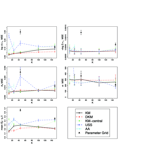
$\widehat{\gamma}_{c}$, measured by the average $\ell_{2}$ distance to the true $\gamma_{c}$. Each prototype method outperforms the regular parameter grid prototype bases, often by large margins, especially for $K=45$. Between the different prototyping methods there does not appear to be a clear winner, though diffusion $K$-means bases achieve the lowest or second-lowest MSE for 4 of the 5 parameters. $K$-means also achieves accurate estimates for each of the parameters, and always beats or ties the $K$-means-central estimates. Both USS and AA yield inaccurate estimates for all parameters except $\langle\log Z_{*}\rangle_{L}$ and $\sigma_{*}$. SSS could not be run on such a large dictionary of SSPs. Overall, small bases achieve better estimates of $\log\langle t_{*}\rangle_{L},A_{V}$ and $\gamma_{\mathrm{c}}$, but this likely will not be the case for real galaxies, whose SFHs are more complicated and diverse than the simulation prescription used.

6 Analysis of SDSS galaxies

Prototyping methods are used to estimate the SFH parameters from the SDSS spectra of a set of 3046 galaxies in SDSS Data Release 6 [Adelman-McCarthy et al. (2008)]. For more detailed information about the data and preprocessing steps, see Richards et al. (2009a). In Figure 8 we plot the estimated $\log\langle t_{*}\rangle_{L}$ versus $\langle\log Z_{*}\rangle_{L}$ for each galaxy using three basis choices: the regular parameter grid of Asari et al. (2007) (Asa07, $K=150$), DKM with $K=45$, and DKM with $K=150$.

Figure 8: Estimates of $\log\langle t_{*}\rangle_{L}$ versus $\langle\log Z_{*}\rangle_{L}$ for a set of 3046 galaxies observed by the SDSS, estimated using STARLIGHT with three different prototype bases. From left to right, bases are as follows: regular parameter grid from Asari et al. (2007) with $K=150$, diffusion $K$-means $K=45$, and diffusion $K$-means $K=150$. Estimates from diffusion $K$-means bases show much less spread in the direction of the well-known age-metallicity degeneracy in galaxy population synthesis studies.

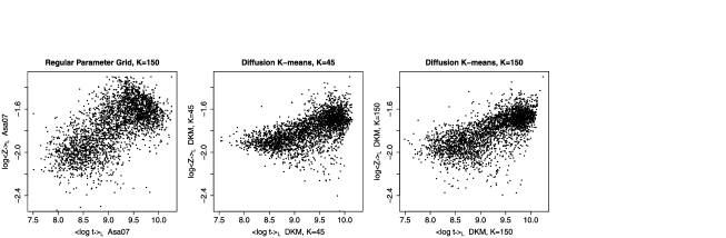
There are several differences in the estimated $\langle\log Z_{*}\rangle_{L}-\log\langle t_{*}\rangle_{L}$ relation for each basis. First, both diffusion $K$-means bases produce estimates that are tightly spread around an increasing trend while the Asa07 estimates are more diffusely spread around such a trend. The direction of discrepancy in the Asa07 estimates from the trend corresponds exactly with the direction of a well-known spectral degeneracy between old, metal-poor and young, metal-rich galaxies [Worthey (1994)]. This suggests that the observed variability along this direction is not due to the physics of these galaxies, but rather is caused by confusion stemming from the choice of basis [in Richards et al. (2009a) we verified that diffusion $K$-means SFH estimates have a decreased age-metallicity degeneracy, using simulated galaxy spectra]. Second, the $K=45$ diffusion $K$-means basis estimates no young, metal-poor galaxies, whereas the other bases do. This suggests that this small number of prototypes is not sufficient to cover the parameter space; particularly, young, metal-poor SSPs have been neglected in the $K=45$ diffusion $K$-means basis. Finally, the overall trend between $\log\langle t_{*}\rangle_{L}$ versus $\langle\log Z_{*}\rangle_{L}$ differs substantially between the regular grid and diffusion $K$-means basis, suggesting that SFH parameter estimates are sensitive to the choice of basis and that downstream cosmological inferences will depend heavily on the basis used.

Recently, we have estimated the SFH parameters for all 781,692 galaxies in the SDSS DR7 [Abazajian (2009)] main sample or LRG sample. This subset of DR7 galaxies was chosen for analysis because it was targeted for spectroscopic observation, and thus has a well defined selection function [Strauss (2002)]. We estimated the parameters using STARLIGHT with a diffusion $K$-means basis of size $K=150$. The computational routines took nearly 5 CPU years to analyze the entire data set, which includes preprocessing of the data, estimating the SFH parameters for each, and compiling the catalog of estimates. The computations were performed in parallel on the 1,000-core high-performance FLUX cluster at the University of Michigan. Results of this analysis are in preparation [Richards and Miller (2011)] and will be published shortly. These SFH estimates will be used to constrain cosmological models that concern the formation and evolution of galaxies and the history and fate of the Universe.

There is also ongoing work into approaches to quantifying the statistical uncertainty in the resulting parameter estimates. This is a critical, but challenging, component. The basic approach to be employed will exploit the massive amount of data by inspecting the amount of variability in parameter estimates in small neighborhoods in the space of galaxy spectra. An additional regression model will be fit, with the parameter estimates as the response, and the spectrum as the predictor. In previous work [Richards et al. (2009b) and Freeman et al. (2009)], we have fit models of exactly this type, using galaxy spectra or colors to predict redshift. As was the case in that work, we will smooth the parameter estimates in the high-dimensional space to obtain an estimator with lower variance. Equally important, this will yield a natural way of estimating the uncertainty in the estimator, by inspecting the variance of the residuals of the regression fit.

7 Conclusions

We have introduced a prototyping approach for the common class of parameter estimation problems where observed data are produced as a constrained linear combination of theoretical model-produced components, and the target parameters are derived from the parameters in the signal model. The usual approach to this type of problem is to use models on a regular grid in parameter space. In this paper we have introduced approaches that use the properties of the theoretical data from the dictionary of components to estimate prototype bases. These approaches include: quantizing the component model data space using $K$-means, selecting prototypes uniformly over the space of theoretical component data, and estimating prototype bases that minimize the reconstruction error of the components.

Our main findings are the following:

• The quantization methods presented in this paper achieve better parameter estimates than the approach of using prototypes from a regular parameter grid, as shown in multiple simulations. The regularization that results from a reduced basis leads to reduced variance in the parameter estimates, without sacrificing accuracy. This is the case because components with similar theoretical data will be indiscernible under the presence of noise, making it crucial that prototypes be spread out evenly in theoretical data space, inducing a large decrease in variance of the target parameter estimates. If bases are too small, then the parameter estimates suffer from large bias because important regions of model space are neglected.

• Standard sparse coding methods are not appropriate for this class of problem. Without the proper constraints, these methods do not find prototypes that are physically-plausible. Even with these constraints, these methods select prototypes around the boundary of the data distribution, which is good for data reconstruction but not for target parameter estimation.

• For a complicated problem in astrophysics—estimating the history of star formation for each galaxy in a large database—we obtain more accurate parameters (in simulations) using the model quantization approach than using regular parameter grids. When applied to the real data, these different prototyping approaches produce markedly different results, showing the importance of prototype basis selection.

References

- Abazajian (2009) {barticle}[author] \bauthor\bsnmAbazajian, \bfnmK. N. et al.\binitsK. N. e. a. (\byear2009). \btitleThe seventh data release of the sloan digital sky survey. \bjournalAstrophysical Journal Supplement Series \bvolume182 \bpages543–558. \bptokimsref \endbibitem
- Adams, Smith and Johnson (1986) {barticle}[author] \bauthor\bsnmAdams, \bfnmJ. B.\binitsJ. B., \bauthor\bsnmSmith, \bfnmM. O.\binitsM. O. and \bauthor\bsnmJohnson, \bfnmP. E.\binitsP. E. (\byear1986). \btitleSpectral mixture modeling: A new analysis of rock and soil types at the Viking Lander 1 site. \bjournalJ. Geophys. Res. \bvolume91 \bpages8098–8112. \bptokimsref \endbibitem
- Adelman-McCarthy et al. (2008) {barticle}[author] \bauthor\bsnmAdelman-McCarthy, \bfnmJ. K.\binitsJ. K. \betalet al. (\byear2008). \btitleThe sixth data release of the sloan digital sky survey. \bjournalAstrophysical Journal Supplement Series \bvolume175 \bpages297–313. \bptokimsref \endbibitem
- Allassonnière, Amit and Trouvé (2007) {barticle}[mr] \bauthor\bsnmAllassonnière, \bfnmS.\binitsS., \bauthor\bsnmAmit, \bfnmY.\binitsY. and \bauthor\bsnmTrouvé, \bfnmA.\binitsA. (\byear2007). \btitleTowards a coherent statistical framework for dense deformable template estimation. \bjournalJ. R. Stat. Soc. Ser. B Stat. Methodol. \bvolume69 \bpages3–29. \biddoi=10.1111/j.1467-9868.2007.00574.x, issn=1369-7412, mr=2301497 \bptokimsref \endbibitem
- Asari et al. (2007) {barticle}[author] \bauthor\bsnmAsari, \bfnmN. V.\binitsN. V., \bauthor\bsnmCid Fernandes, \bfnmR.\binitsR., \bauthor\bsnmStasińska, \bfnmG.\binitsG., \bauthor\bsnmTorres-Papaqui, \bfnmJ. P.\binitsJ. P., \bauthor\bsnmMateus, \bfnmA.\binitsA., \bauthor\bsnmSodré, \bfnmL.\binitsL., \bauthor\bsnmSchoenell, \bfnmW.\binitsW. and \bauthor\bsnmGomes, \bfnmJ. M.\binitsJ. M. (\byear2007). \btitleThe history of star-forming galaxies in the sloan digital sky survey. \bjournalMonthly Notices of the Royal Astronomical Society \bvolume381 \bpages263–279. \bptokimsref \endbibitem
- Babak et al. (2006) {barticle}[author] \bauthor\bsnmBabak, \bfnmS.\binitsS., \bauthor\bsnmBalasubramanian, \bfnmR.\binitsR., \bauthor\bsnmChurches, \bfnmD.\binitsD., \bauthor\bsnmCokelaer, \bfnmT.\binitsT. and \bauthor\bsnmSathyaprakash, \bfnmBS\binitsB. (\byear2006). \btitleA template bank to search for gravitational waves from inspiralling compact binaries: I. Physical models. \bjournalClassical Quantum Gravity \bvolume23 \bpages5477–5504. \bptokimsref \endbibitem
- Bayarri et al. (2007) {barticle}[mr] \bauthor\bsnmBayarri, \bfnmM. J.\binitsM. J., \bauthor\bsnmBerger, \bfnmJ. O.\binitsJ. O., \bauthor\bsnmCafeo, \bfnmJ.\binitsJ., \bauthor\bsnmGarcia-Donato, \bfnmG.\binitsG., \bauthor\bsnmLiu, \bfnmF.\binitsF., \bauthor\bsnmPalomo, \bfnmJ.\binitsJ., \bauthor\bsnmParthasarathy, \bfnmR. J.\binitsR. J., \bauthor\bsnmPaulo, \bfnmR.\binitsR., \bauthor\bsnmSacks, \bfnmJ.\binitsJ. and \bauthor\bsnmWalsh, \bfnmD.\binitsD. (\byear2007). \btitleComputer model validation with functional output. \bjournalAnn. Statist. \bvolume35 \bpages1874–1906. \biddoi=10.1214/009053607000000163, issn=0090-5364, mr=2363956 \bptokimsref \endbibitem
- Bica (1988) {barticle}[author] \bauthor\bsnmBica, \bfnmE.\binitsE. (\byear1988). \btitlePopulation synthesis in galactic nuclei using a library of star clusters. \bjournalAstronomy and Astrophysics \bvolume195 \bpages76–92. \bptokimsref \endbibitem
- Boyd and Vandenberghe (2004) {bbook}[mr] \bauthor\bsnmBoyd, \bfnmStephen\binitsS. and \bauthor\bsnmVandenberghe, \bfnmLieven\binitsL. (\byear2004). \btitleConvex Optimization. \bpublisherCambridge Univ. Press, \baddressCambridge. \bidmr=2061575 \bptokimsref \endbibitem
- Bruzual and Charlot (2003) {barticle}[author] \bauthor\bsnmBruzual, \bfnmG.\binitsG. and \bauthor\bsnmCharlot, \bfnmS.\binitsS. (\byear2003). \btitleStellar population synthesis at the resolution of 2003. \bjournalMonthly Notices of the Royal Astronomical Society \bvolume344 \bpages1000–1028. \bptokimsref \endbibitem
- Cardelli, Clayton and Mathis (1989) {barticle}[author] \bauthor\bsnmCardelli, \bfnmJ. A.\binitsJ. A., \bauthor\bsnmClayton, \bfnmG. C.\binitsG. C. and \bauthor\bsnmMathis, \bfnmJ. S.\binitsJ. S. (\byear1989). \btitleThe relationship between infrared, optical, and ultraviolet extinction. \bjournalAstrophysical Journal \bvolume345 \bpages245–256. \bptokimsref \endbibitem
- Chen et al. (2009) {barticle}[author] \bauthor\bsnmChen, \bfnmX. Y.\binitsX. Y., \bauthor\bsnmLiang, \bfnmY. C.\binitsY. C., \bauthor\bsnmHammer, \bfnmF.\binitsF., \bauthor\bsnmZhao, \bfnmY. H.\binitsY. H. and \bauthor\bsnmZhong, \bfnmG. H.\binitsG. H. (\byear2009). \btitleStellar population analysis on local infrared-selected galaxies. \bjournalAstronomy and Astrophysics \bvolume495 \bpages457–469. \bptokimsref \endbibitem
- Cid Fernandes et al. (2001) {barticle}[author] \bauthor\bsnmCid Fernandes, \bfnmR.\binitsR., \bauthor\bsnmSodré, \bfnmL.\binitsL., \bauthor\bsnmSchmitt, \bfnmH. R.\binitsH. R. and \bauthor\bsnmLeão, \bfnmJ. R. S.\binitsJ. R. S. (\byear2001). \btitleA probabilistic formulation for empirical population synthesis: Sampling methods and tests. \bjournalMonthly Notices of the Royal Astronomical Society \bvolume325 \bpages60–76. \bptokimsref \endbibitem
- Cid Fernandes et al. (2004) {barticle}[author] \bauthor\bsnmCid Fernandes, \bfnmR.\binitsR., \bauthor\bsnmGu, \bfnmQ.\binitsQ., \bauthor\bsnmMelnick, \bfnmJ.\binitsJ., \bauthor\bsnmTerlevich, \bfnmE.\binitsE., \bauthor\bsnmTerlevich, \bfnmR.\binitsR., \bauthor\bsnmKunth, \bfnmD.\binitsD., \bauthor\bsnmRodrigues Lacerda, \bfnmR.\binitsR. and \bauthor\bsnmJoguet, \bfnmB.\binitsB. (\byear2004). \btitleThe star formation history of Seyfert 2 nuclei. \bjournalMonthly Notices of the Royal Astronomical Society \bvolume355 \bpages273–296. \bptokimsref \endbibitem
- Cid Fernandes et al. (2005) {barticle}[author] \bauthor\bsnmCid Fernandes, \bfnmR.\binitsR., \bauthor\bsnmMateus, \bfnmA.\binitsA., \bauthor\bsnmSodré, \bfnmL.\binitsL., \bauthor\bsnmStasińska, \bfnmG.\binitsG. and \bauthor\bsnmGomes, \bfnmJ. M.\binitsJ. M. (\byear2005). \btitleSemi-empirical analysis of Sloan Digital Sky Survey galaxies. I. Spectral synthesis method. \bjournalMonthly Notices of the Royal Astronomical Society \bvolume358 \bpages363–378. \bptokimsref \endbibitem
- Clark et al. (2004) {barticle}[author] \bauthor\bsnmClark, \bfnmB. E.\binitsB. E., \bauthor\bsnmBus, \bfnmS. J.\binitsS. J., \bauthor\bsnmRivkin, \bfnmA. S.\binitsA. S., \bauthor\bsnmMcConnochie, \bfnmT.\binitsT., \bauthor\bsnmSanders, \bfnmJ.\binitsJ., \bauthor\bsnmShah, \bfnmS.\binitsS., \bauthor\bsnmHiroi, \bfnmT.\binitsT. and \bauthor\bsnmShepard, \bfnmM.\binitsM. (\byear2004). \btitleE-type asteroid spectroscopy and compositional modeling. \bjournalJ. Geophys. Res. \bvolume109 \bpages2001. \bptokimsref \endbibitem
- Coifman and Lafon (2006) {barticle}[mr] \bauthor\bsnmCoifman, \bfnmRonald R.\binitsR. R. and \bauthor\bsnmLafon, \bfnmStéphane\binitsS. (\byear2006). \btitleDiffusion maps. \bjournalAppl. Comput. Harmon. Anal. \bvolume21 \bpages5–30. \biddoi=10.1016/j.acha.2006.04.006, issn=1063-5203, mr=2238665 \bptokimsref \endbibitem
- Cutler and Breiman (1994) {barticle}[mr] \bauthor\bsnmCutler, \bfnmAdele\binitsA. and \bauthor\bsnmBreiman, \bfnmLeo\binitsL. (\byear1994). \btitleArchetypal analysis. \bjournalTechnometrics \bvolume36 \bpages338–347. \bidissn=0040-1706, mr=1304898 \bptokimsref \endbibitem
- Freeman et al. (2009) {barticle}[author] \bauthor\bsnmFreeman, \bfnmP. E.\binitsP. E., \bauthor\bsnmNewman, \bfnmJ. A.\binitsJ. A., \bauthor\bsnmLee, \bfnmA. B.\binitsA. B., \bauthor\bsnmRichards, \bfnmJ. W.\binitsJ. W. and \bauthor\bsnmSchafer, \bfnmC. M.\binitsC. M. (\byear2009). \btitlePhotometric redshift estimation using spectral connectivity analysis. \bjournalMonthly Notices of the Royal Astronomical Society \bvolume398 \bpages2012–2021. \bptokimsref \endbibitem
- Geman and Hwang (1982) {barticle}[mr] \bauthor\bsnmGeman, \bfnmStuart\binitsS. and \bauthor\bsnmHwang, \bfnmChii-Ruey\binitsC.-R. (\byear1982). \btitleNonparametric maximum likelihood estimation by the method of sieves. \bjournalAnn. Statist. \bvolume10 \bpages401–414. \bidissn=0090-5364, mr=0653512 \bptokimsref \endbibitem
- Grant and Boyd (2010) {bmisc}[author] \bauthor\bsnmGrant, \bfnmM.\binitsM. and \bauthor\bsnmBoyd, \bfnmS.\binitsS. (\byear2010). \bhowpublishedCVX: Matlab Software for Disciplined Convex Programming, version 1.21. Available at http://cvxr.com/cvx. \bptokimsref \endbibitem
- Grenander (1981) {bbook}[mr] \bauthor\bsnmGrenander, \bfnmUlf\binitsU. (\byear1981). \btitleAbstract Inference. \bpublisherWiley, \baddressNew York. \bidmr=0599175 \bptokimsref \endbibitem
- Hapke and Wells (1981) {barticle}[author] \bauthor\bsnmHapke, \bfnmB.\binitsB. and \bauthor\bsnmWells, \bfnmE.\binitsE. (\byear1981). \btitleBidirectional reflectance spectroscopy 2. Experiments and observations. \bjournalJ. Geophys. Res. \bvolume86 \bpages3055–3060. \bptokimsref \endbibitem
- Lafon and Lee (2006) {barticle}[author] \bauthor\bsnmLafon, \bfnmS.\binitsS. and \bauthor\bsnmLee, \bfnmA. B.\binitsA. B. (\byear2006). \btitleDiffusion maps and coarse-graining: A unified framework for dimensionality reduction, graph partitioning, and data set parameterization. \bjournalIEEE Transactions on Pattern Analysis and Machine Intelligence \bvolume28 \bpages1393. \bptokimsref \endbibitem
- Lawson and Hanson (1995) {bbook}[author] \bauthor\bsnmLawson, \bfnmC. L.\binitsC. L. and \bauthor\bsnmHanson, \bfnmR. J.\binitsR. J. (\byear1995). \btitleSolving Least Squares Problems. \bpublisherSIAM, \baddressPhiladelphia, PA. \bidmr=1349828 \bptokimsref \endbibitem
- Lee and Seung (2001) {barticle}[author] \bauthor\bsnmLee, \bfnmD. D.\binitsD. D. and \bauthor\bsnmSeung, \bfnmH. S.\binitsH. S. (\byear2001). \btitleAlgorithms for non-negative matrix factorization. \bjournalAdv. Neural Inf. Process. Syst. \bpages556–562. \bptokimsref \endbibitem
- Levy and Steinberg (2010) {barticle}[mr] \bauthor\bsnmLevy, \bfnmSigal\binitsS. and \bauthor\bsnmSteinberg, \bfnmDavid M.\binitsD. M. (\byear2010). \btitleComputer experiments: A review. \bjournalAStA Adv. Stat. Anal. \bvolume94 \bpages311–324. \biddoi=10.1007/s10182-010-0147-9, issn=1863-8171, mr=2753331 \bptokimsref \endbibitem
- Meinicke and Ritter (2002) {barticle}[author] \bauthor\bsnmMeinicke, \bfnmP.\binitsP. and \bauthor\bsnmRitter, \bfnmH.\binitsH. (\byear2002). \btitleQuantizing density estimators. \bjournalAdv. Neural Inf. Process. Syst. \bvolume2 \bpages825–832. \bptokimsref \endbibitem
- Obozinski et al. (2011) {barticle}[author] \bauthor\bsnmObozinski, \bfnmG.\binitsG., \bauthor\bsnmWainwright, \bfnmM. J.\binitsM. J., \bauthor\bsnmJordan, \bfnmM. I.\binitsM. I. (\byear2011). \btitleSupport union recovery in high-dimensional multivariate regression. \bjournalAnn. Statist. \bvolume39 \bpages1–47. \bidmr=2797839 \bptokimsref \endbibitem
- Olshausen et al. (1996) {barticle}[author] \bauthor\bsnmOlshausen, \bfnmB. A.\binitsB. A. \betalet al. (\byear1996). \btitleEmergence of simple-cell receptive field properties by learning a sparse code for natural images. \bjournalNature \bvolume381 \bpages607–609. \bptokimsref \endbibitem
- Owen and Sathyaprakash (1999) {barticle}[author] \bauthor\bsnmOwen, \bfnmB. J.\binitsB. J. and \bauthor\bsnmSathyaprakash, \bfnmBS\binitsB. (\byear1999). \btitleMatched filtering of gravitational waves from inspiraling compact binaries: Computational cost and template placement. \bjournalPhys. Rev. D \bvolume60 \bpages22002. \bptokimsref \endbibitem
- Paatero and Tapper (1994) {barticle}[author] \bauthor\bsnmPaatero, \bfnmP.\binitsP. and \bauthor\bsnmTapper, \bfnmU.\binitsU. (\byear1994). \btitlePositive matrix factorization: A non-negative factor model with optimal utilization of error estimates of data values. \bjournalEnvironmetrics \bvolume5 \bpages111–126. \bptokimsref \endbibitem
- Panter et al. (2007) {barticle}[author] \bauthor\bsnmPanter, \bfnmB.\binitsB., \bauthor\bsnmJimenez, \bfnmR.\binitsR., \bauthor\bsnmHeavens, \bfnmA. F.\binitsA. F. and \bauthor\bsnmCharlot, \bfnmS.\binitsS. (\byear2007). \btitleThe star formation histories of galaxies in the sloan digital sky survey. \bjournalMonthly Notices of the Royal Astronomical Society \bvolume378 \bpages1550–1564. \bptokimsref \endbibitem
- Pelat (1997) {barticle}[author] \bauthor\bsnmPelat, \bfnmD.\binitsD. (\byear1997). \btitleA new method to solve stellar population synthesis problems with the use of a data base. \bjournalMonthly Notices of the Royal Astronomical Society \bvolume284 \bpages365–375. \bptokimsref \endbibitem
- Richards and Miller (2011) {bmisc}[author] \bauthor\bsnmRichards, \bfnmJ. W.\binitsJ. W. and \bauthor\bsnmMiller, \bfnmC. J.\binitsC. J. (\byear2011). \bhowpublishedStar formation history estimates for SDSS DR6. Unpublished manuscript, Carnegie Mellon Univ., Pittsburgh, PA. \bptokimsref \endbibitem
- Richards et al. (2009a) {barticle}[author] \bauthor\bsnmRichards, \bfnmJ. W.\binitsJ. W., \bauthor\bsnmFreeman, \bfnmP. E.\binitsP. E., \bauthor\bsnmLee, \bfnmA. B.\binitsA. B. and \bauthor\bsnmSchafer, \bfnmC. M.\binitsC. M. (\byear2009a). \btitleAccurate parameter estimation for star formation history in galaxies using SDSS spectra. \bjournalMonthly Notices of the Royal Astronomical Society \bvolume399 \bpages1044–1057. \bptokimsref \endbibitem
- Richards et al. (2009b) {barticle}[author] \bauthor\bsnmRichards, \bfnmJ. W.\binitsJ. W., \bauthor\bsnmFreeman, \bfnmP. E.\binitsP. E., \bauthor\bsnmLee, \bfnmA. B.\binitsA. B. and \bauthor\bsnmSchafer, \bfnmC. M.\binitsC. M. (\byear2009b). \btitleExploiting low-dimensional structure in astronomical spectra. \bjournalAstrophysical Journal \bvolume691 \bpages32–42. \bptokimsref \endbibitem
- Roberts et al. (1998) {barticle}[author] \bauthor\bsnmRoberts, \bfnmDA\binitsD., \bauthor\bsnmGardner, \bfnmM.\binitsM., \bauthor\bsnmChurch, \bfnmR.\binitsR., \bauthor\bsnmUstin, \bfnmS.\binitsS., \bauthor\bsnmScheer, \bfnmG.\binitsG. and \bauthor\bsnmGreen, \bfnmRO\binitsR. (\byear1998). \btitleMapping chaparral in the Santa Monica Mountains using multiple endmember spectral mixture models. \bjournalRemote Sensing of Environment \bvolume65 \bpages267–279. \bptokimsref \endbibitem
- Sabuncu, Balci and Golland (2008) {bmisc}[author] \bauthor\bsnmSabuncu, \bfnmM.\binitsM., \bauthor\bsnmBalci, \bfnmS.\binitsS. and \bauthor\bsnmGolland, \bfnmP.\binitsP. (\byear2008). \bhowpublishedDiscovering modes of an image population through mixture modeling. In Proceedings MICCAI 2008: Medical Image Computing and Computer-Assisted Intervention–MICCAI 381–389. Springer, Berlin. \bptokimsref \endbibitem
- Santner, Williams and Notz (2003) {bbook}[mr] \bauthor\bsnmSantner, \bfnmThomas J.\binitsT. J., \bauthor\bsnmWilliams, \bfnmBrian J.\binitsB. J. and \bauthor\bsnmNotz, \bfnmWilliam I.\binitsW. I. (\byear2003). \btitleThe Design and Analysis of Computer Experiments. \bpublisherSpringer, \baddressNew York. \bidmr=2160708 \bptokimsref \endbibitem
- Stone (2002) {barticle}[mr] \bauthor\bsnmStone, \bfnmEmily\binitsE. (\byear2002). \btitleExploring archetypal dynamics of pattern formation in cellular flames. \bjournalPhys. D \bvolume161 \bpages163–186. \biddoi=10.1016/S0167-2789(01)00361-X, issn=0167-2789, mr=1878533 \bptokimsref \endbibitem
- Strauss (2002) {barticle}[author] \bauthor\bsnmStrauss, \bfnmM. A. et. al\binitsM. A. e. a. (\byear2002). \btitleSpectroscopic target selection in the sloan digital sky survey: The main galaxy sample. \bjournalAstronomical Journal \bvolume124 \bpages1810–1824. \bptokimsref \endbibitem
- Worthey (1994) {barticle}[author] \bauthor\bsnmWorthey, \bfnmG.\binitsG. (\byear1994). \btitleComprehensive stellar population models and the disentanglement of age and metallicity effects. \bjournalAstrophysical Journal Supplement Series \bvolume95 \bpages107–149. \bptokimsref \endbibitem
- York et al. (2000) {barticle}[author] \bauthor\bsnmYork, \bfnmD. G.\binitsD. G. \betalet al. (\byear2000). \btitleThe sloan digital sky survey: Technical summary. \bjournalAstronomical Journal \bvolume120 \bpages1579–1587. \bptokimsref \endbibitem