g-Factor anisotropy of hole quantum wires induced by the Rashba interaction

Abstract

We present calculations of the g factors for the lower conductance steps of 3D hole quantum wires. Our results prove that the anisotropy with magnetic field orientation, relative to the wire, originates in the Rashba spin-orbit coupling. We also analyze the relevance of the deformation, as the wire evolves from 3D towards a flat 2D geometry. For high enough wire deformations, the perpendicular g factors are greatly quenched by the Rashba interaction. On the contrary, parallel g factors are rather insensistive to the Rashba interaction, resulting in a high g factor anisotropy. For low deformations we find a more irregular behavior which hints at a sample dependent scenario.

I Introduction

Spin-orbit interactions in semiconductor materials offer interesting possibilities of spin control in nanostructures.win03 Among them, the Rashba interaction that originates in externally applied electric fields is most promising due to its tunability. In this work we prove that the Rashba interaction is an important source of spin anisotropy in hole quantum wires. This anisotropy manifests in large differences between the energy splittings for magnetic fields parallel and perpendicular to the wire.dan97 ; dan06 ; kod08 ; klo09 Our calculations show that in the presence of Rashba interaction the perpendicular field becomes much less effective in generating spin splittings than the parallel one. This effect is favored by the deformation of the quantum wire, i.e., anisotropy increases when the wire evolves from 3D towards a more flat quasi 2D geometry.

In semiconductor hole systems like p-type GaAs nanostructures transport is mediated by holes in the valence bands. As compared to electrons, holes are characterized by a spin 3/2, besides a sign difference in charge. The corresponding fourfold discrete space is a source of qualitative differences with respect to the more usual twofold spin of electrons. In 2D hole gases different splittings for normal and in-plane fields have been observed, as well as for different in-plane orientations.win00 By further confining the hole gas it is possible to generate nanostructures with the shape of quantum wires. In this case, the splitting varies, in principle, with both wire and magnetic field orientations.dan06 ; kod08 ; klo09

There are few theoretical analysis of the spin splittings in hole quantum wires.gol95 ; har06 ; cso07 Although the Rashba interaction was usually not taken into account, this situation changed in some recent works.che11 ; qua10 Indeed, Quay et al.qua10 have observed the formation of a spin-orbit gap induced by the combined action of magnetic field and Rashba coupling in a hole quantum wire, while Chesi et al.che11 have studied, both experimentally and theoretically, the spin resolved transmission of a quantum point contact fabricated in a 2D hole gas. In the latter, the Rashba interaction is shown to favor a band crossing at finite wavenumber that can be manipulated with an external magnetic field. In agreement with our results, this crossing is obtained in a multiband description of the hole states. It can also be explained within a restricted single band description adding a cubic Rashba term.

In this work we have focussed our attention on the structure-inversion-asymmetry (Rashba) splitting since this is known to be the dominant source of spin-orbit coupling in GaAs. The bulk-inversion-asymmetry (Dresselhaus) is much smaller and has a minimal effect on the energy bands.qua10 ; win00 We will show that in a hole quantum wire oriented along $x^{\prime}$ the Rashba interaction due to asymmetry in the growth direction ($z^{\prime}$) causes a large difference between parallel ($x^{\prime}$) and perpendicular ($y^{\prime}$) g factors of the wire, as deduced from the $B$-induced splittings of the conductance steps. This anisotropy is due to the quenching of the splitting when $B$ is along $y^{\prime}$ and the wire flatness is large. For smaller deformations the situation is less clear due to a non monotonous evolution of the splittings that may result in a sample-dependent scenario.

II Model

We describe the anisotropic kinetic energies ${\cal H}^{\it(kin)}$ of the holes in a 4-band kp model. Introducing a spin discrete index $\eta=3/2,\dots,-3/2$ and following the notation of Ref. [win03, ] the diagonal terms read

$${\cal H}^{\it(kin)}_{\eta\eta}=-\frac{\hbar^{2}}{2m_{0}}\left[(\gamma_{1}+c_{\eta}\gamma_{2})k_{\parallel}^{2}+(\gamma_{1}-2c_{\eta}\gamma_{2})k_{z}^{2}\right]\;,$$ (1)

where $c_{\pm 3/2}=1$ and $c_{\pm 1/2}=-1$. In Eq. (1) $\gamma_{1}$ and $\gamma_{2}$ are the kp parameters, $\vec{k}$ is the 3D wavenumber and we have also defined $k_{\parallel}^{2}=k_{x}^{2}+k_{y}^{2}$. The nondiagonal kinetic terms are

$${\cal H}^{\it(kin)}_{+\frac{3}{2},+\frac{1}{2}} = \frac{\hbar^{2}}{m_{0}}\sqrt{3}\,\gamma_{3}\,k_{-}k_{z}\;,$$

$${\cal H}^{\it(kin)}_{+\frac{3}{2},-\frac{1}{2}} = \frac{\hbar^{2}}{2m_{0}}\sqrt{3}(\gamma_{2}\hat{K}-2i\gamma_{3}k_{x}k_{y})\;,$$

$${\cal H}^{\it(kin)}_{+\frac{1}{2},-\frac{3}{2}} = {\cal H}^{\it(kin)}_{+\frac{3}{2},-\frac{1}{2}}\;,$$

$${\cal H}^{\it(kin)}_{-\frac{1}{2},-\frac{3}{2}} = -{\cal H}^{\it(kin)}_{+\frac{3}{2},+\frac{1}{2}}\;,$$ (2)

where $k_{\pm}=k_{x}\pm ik_{y}$ and $\hat{K}=k_{x}^{2}-k_{y}^{2}$. We only refer to contributions in the upper triangle of matrix ${\cal H}^{\it(kin)}_{\eta\eta^{\prime}}$ since the remaining ones can be inferred from the Hermitian character of the matrix. In all calculations discussed below we have used numerical values for the kp parameters $\gamma$’s corresponding to GaAs.win03

The wire confinement is represented by a deformed 2D harmonic oscillator. Assuming the wire is oriented along $x^{\prime}$ while transverse and growth directions are given by $y^{\prime}$ and $z^{\prime}$, respectively, it is

$${\cal H}^{\it(conf)}=-\frac{1}{2}m_{0}\omega_{0}^{2}({y^{\prime}}^{2}+a{z^{\prime}}^{2})\;.$$ (3)

The adimensional parameter $a$ of Eq. (3), corresponding to the ratio of confinement strengths in $z^{\prime}$ and $y^{\prime}$, controls the flatness or 2D character of the wire. The direct coupling with the magnetic field $\vec{B}$ is given by the Zeeman term

$${\cal H}^{(Z)}=-2\kappa\mu_{B}\vec{B}\cdot\vec{J}\;,$$ (4)

where $\kappa$ is a kp parameter, $\mu_{B}$ represents the Bohr magneton and $\vec{J}$ is the angular momentum operator for a spin 3/2. Finally, the Rashba interaction is described by

$${\cal H}^{(R)}=(\vec{k}\times\vec{\cal R})\cdot\vec{J}\;,$$ (5)

where we defined a vector constant $\vec{\cal R}\equiv\alpha\vec{\cal E}$, related to the effective electric field $\vec{\cal E}$ and kp parameter $\alpha$.win03 We shall treat $\vec{\cal R}$ as a two-parameter vector with dominant component along the growth direction, i.e., $\vec{\cal R}={\cal R}_{z^{\prime}}\hat{u}_{z^{\prime}}+{\cal R}_{y^{\prime}}\hat{u}_{y^{\prime}}$ with ${\cal R}_{z^{\prime}}>{\cal R}_{y^{\prime}}$.

In the presence of a magnetic field, the orbital effects of the field are taken into account by means of the substitution $\vec{k}\to-i\nabla-\frac{e}{\hbar c}\vec{A}$ with the vector potential $\vec{A}=(-yB_{z}+zB_{y},-B_{x}z/2,B_{x}y/2)$. In this process, Hermiticity is enforced in the cross terms by using the symmetrized forms, such as $k_{x}k_{y}\to(k_{x}k_{y}+k_{y}k_{x})/2$. Summarizing all contributions the total Hamiltonian reads

$${\cal H}\equiv{\cal H}^{\it(kin)}+{\cal H}^{\it(conf)}+{\cal H}^{(Z)}+{\cal H}^{(R)}\;.$$ (6)

The wire Hamiltonian eigenvalues can be labelled with $q$, a real number representing the longitudinal momentum and an index $I=1,2,\dots$ as

$${\cal H}(q)|Iq\rangle=\varepsilon_{I}(q)|Iq\rangle\;,$$ (7)

where $\varepsilon_{I}(q)$ are the discrete energy bands of the nanostructure. The eigenvalues are ordered as $\varepsilon_{1}(q)\geq\varepsilon_{2}(q)\geq\dots$ since the spectrum is not bounded from below due to the negative kinetic terms.

We have obtained the solutions of the eigenvalue problem given by Eq. (7) by discretizing in harmonic oscillator states for the two transverse oscillators along $y^{\prime}$ and $z^{\prime}$,

$$|Iq\rangle=\sum_{nm\eta}{C_{nm\eta}^{(Iq)}}\,|nm\eta\rangle\;,$$ (8)

where $n,m=0,1,\dots$ represent the number of quanta in each oscillator, respectively. The resulting matrix eigenvalue problem reads

$$\sum_{nm\eta}{\langle n^{\prime}m^{\prime}\eta^{\prime}|{\cal H}(q)|nm\eta\rangle\,C^{(Iq)}_{nm\eta}=\varepsilon_{I}(q)\,C^{(Iq)}_{n^{\prime}m^{\prime}\eta^{\prime}}}\;.$$ (9)

In practice the number of oscillator states in expansion Eq. (8) can be truncated once convergence of the results is ensured. The results shown below are well converged and they have been obtained including the lower 20 oscillator states in each direction. In Appendix B a precise discussion on the relevance of the basis truncation is given.

III Results and discussion

As illustrative examples, Fig. 1 displays the energy bands of selected cases. As is well known, the Rashba interaction causes a characteristic band structure easily recognizable by the pairs of subbands crossing at $q=0$ and with maxima at opposite $q$ values (left panel). These maxima correspond to band energy minima for the case of electrons. In the presence of a magnetic field, when this points along the wire ($x^{\prime}$, central panel), an anticrossing of the bands appears at $q=0$. This anticrossing may lead to anomalous conductance steps, similar to those recently measured in Ref. qua10, . In Fig. 1 this behavior can be seen for $(E,q)\approx(-11\hbar\omega_{0},0)$. For $B$ in the transverse direction ($y^{\prime}$, right panel) the band crossings persist, but the two central maxima for each pair of bands are shifted differently in energy, the band structure becoming asymmetric with respect to $q$ inversion.

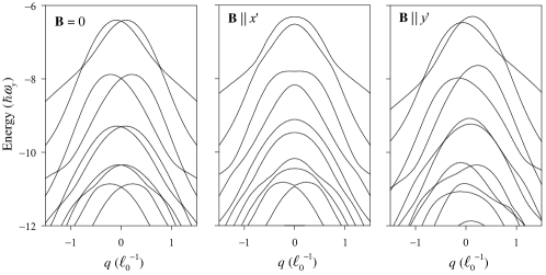
Figure 1: Energy bands for $a=64$, ${\cal R}_{z^{\prime}}=2.6\hbar\omega_{0}\ell_{0}$ and ${\cal R}_{y^{\prime}}=0$. Left panel is for $B=0$ while center and right ones are for $\mu_{B}B=0.1\hbar\omega_{0}$ in the parallel and transverse directions, respectively. The wire is oriented along $(-2,3,3)$ and the growth direction is $(3,1,1)$.

The $B$-induced modifications of the band structure, as seen in Fig. 1, cause a change in the conductance of the wire. This modification of the conductance, in the limit of weak magnetic field, is conveniently summarized by a number called the g factor of each conductance split level. At $B=0$, time reversal invariance of the system causes the conductance $G$ to increase in steps of $2G_{0}$ as the Fermi energy of the leads is reduced, where $G_{0}=e^{2}/h$ is the conductance quantum. The evolution of the wire conductance with energy can be understood if we imagine a horizontal line, indicating the position of the Fermi energy, in the left panel of Fig. 1; as this line is moved to lower energies it sweeps the band maxima always in pairs, each maxima corresponding to an increase of $G_{0}$ in the conductance for hole transport. The result is the typical staircase conductance, with step heights of $2G_{0}$. A similar procedure for the central and right panels of Fig. 1 convince ourselves that intermediate half steps in conductance are caused by the magnetic field. They are smaller than the full steps and proportional to the intensity of the magnetic field.

The scenario we have just sketched is explicitly shown in Fig. 2, highlighting the conductance half steps at odd multiples of $G_{0}$. Notice that the energy span varies for each specific conductance half step. In the limit of weak magnetic fields we can conveniently summarize the $B$-induced $N$th half step in the conductance, appearing between steps at $2(N-1)G_{0}$ and $2NG_{0}$, in terms of a single number called the g factor. As this number depends on the conductance step and the magnetic field orientation, we use the notation $g^{(N)}_{\parallel}$ and $g^{(N)}_{\perp}$ to indicate the g factor of the $N$th step, for $B$ along $x^{\prime}$ and $y^{\prime}$, respectively. Of course, other orientations are in principle possible, but we will restrict first to these two as they are the relevant ones in the measurements of spin hole anisotropy. In Appendix A we will briefly mention the behavior for $z^{\prime}$-oriented field.

Our precise definition of the parallel-field g-factor is

$$g^{(N)}_{\parallel}=\frac{\Delta^{(N)}_{\parallel}}{3\mu_{B}B}\;$$ (10)

where $\Delta_{\parallel}^{(N)}$ is the energy range for the $N$th half step in a magnetic field $B$. In Eq. (10), the factor 3 in the denominator is introduced by convention.gg The definition of $g^{(N)}_{\perp}$, for magnetic field along $y^{\prime}$, is obtained simply replacing $\Delta_{\parallel}^{(N)}$ by $\Delta_{\perp}^{(N)}$ in Eq. (10).

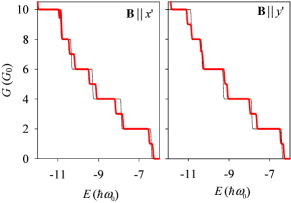
Figure 2: (Color online) Conductance traces for the band structure in parallel and perpendicular magnetic fields of Fig. 1. For comparison, the $B=0$ conductance is displayed as a thin line.

Figure 3 displays the perpendicular (lower row) and parallel (upper row) g factors for the lower conductance steps, as a function of the wire deformation $a$ and for different values of the Rashba coupling ${\cal R}_{z^{\prime}}$. These are the main results of our work. They were obtained for a specific wire orientation and direction of crystallographic growth ($z^{\prime}$) taken from the experimental works of Danneau et al.dan06 and Koduvayur et al.kod08 We have checked, however, that a qualitatively similar influence of the Rashba intensity and confinement deformation are obtained assuming other arbitrary orientations. The g factors show a general tendency to decrease as $a$ increases, except for smaller deformations ($a<100$) for which $g$ may increase or even show irregular behavior in some cases. Focussing first on $g_{\parallel}$, we notice that this component does not change significantly when the Rashba intensity increases, specially at large $a$’s, for which the results are almost overlapping in the upper panels of Fig. 3. Very remarkably, however, for magnetic field in the perpendicular direction small variations in ${\cal R}_{z^{\prime}}$ are enough to strongly modify the values of $g_{\perp}$. This is more clearly seen in Figure 4, which displays the dependence with Rashba coupling intensity of the g factors.

There is a general Rashba-induced quenching of $g_{\perp}^{(N)}$ in Figs. 3 and 4, quite conspicuous for $N=4$ and 5. This effect is so strong that it can reverse the relative importance of $g_{\parallel}$ and $g_{\perp}$; from $g_{\perp}>g_{\parallel}$ when ${\cal R}_{z^{\prime}}=0$ to $g_{\perp}<<g_{\parallel}$ for increasing ${\cal R}_{z^{\prime}}$ ($>2.5\hbar\omega_{0}\ell_{0}$, Fig. 4). With the chosen values of ${\cal R}_{z^{\prime}}$ we even find a range of $a$’s for which $g_{\perp}^{(5)}$ essentially vanishes. It is interesting to point out that a similar quenching of conductance plateaus in transverse field was discussed in Ref. ser05, for parabolic wires with electron conduction, as opposed to the present hole conduction. In both cases the Rashba spin-orbit coupling is the underlying mechanism.

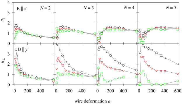
Figure 3: (Color online) Parallel and perpendicular g factors as a function of wire deformation for different values of the Rashba strength: ${\cal R}_{z^{\prime}}=0$ (circles), $1.5\hbar\omega_{0}\ell_{0}$ (triangles) and $2.6\hbar\omega_{0}\ell_{0}$ (squares). Upper and lower rows are for parallel and perpendicular fields while columns from left to right correspond to increasing conductance half step $N$ (see text). The results for $N=1$ are not shown due to their similarity with the displayed $N=2$ case. The orientation of the wire is the same of Fig. 1.

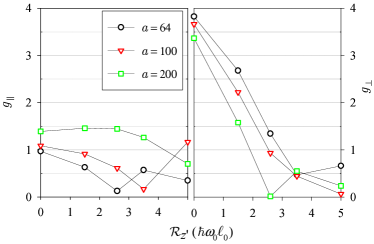
Figure 4: (Color online) Parallel (left) and perpendicular (right) g factors as a function of Rashba coupling intensity for different values of the deformation $a$. The results correspond to the $N=5$ conductance half step.

Turning to the comparison with experiments, this is somewhat complicate due to the sample dependence. In general, however, a large g-factor anisotropy between parallel and perpendicular orientations has indeed been observed in Refs. dan06, ; kod08, ; klo09, . This was generally attributed to a preferential orientation of the spins along the wire for strong confinements. Our results prove with detailed calculations that the Rashba interaction for holes is the specific mechanism allowing the appearance of this anisotropy. As this interaction is sample dependent and may vary with external field, our results also predict that the hole g factors may be tunable to a certain degree, what may be relevant for spintronic applications. The experimental values of wire deformation $a$ are somewhat uncertain in general, which is an additional source of difficulty for comparison. In general, however, experimental wire deformations are $a<100$, which in our calculations corresponds to a regime with rather large fluctuations (Fig. 3). Only for larger $a$’s the value of $g_{\perp}^{(N)}$ is consistently below $g_{\parallel}^{(N)}$ at high enough ${\cal R}_{z^{\prime}}$. We believe that detailed comparison in this regime is quite involved due to the fluctuations. On the other hand, these sharp variations of $g_{\parallel}$ in the small-$a$ regime and of $g_{\perp}$ at all $a$’s can be seen as a manifestation of magnetoconductance tunability via the Rashba coupling.

IV A two-band model

A more transparent physical interpretation, complementing the above numerical results, can be obtained in a simplified model based on only two bands. Focussing on the $I$-th intermediate half step having conductance $IG_{0}$, with $I=1,3,\dots$, we select the two states $I$ and $I+1$ at a given $q$, $\{|Iq\rangle_{0},|(I+1)q\rangle_{0}\}$, where the zero subscript is indicating absence of a magnetic field. These two states are the basis in which the effect of the magnetic field in different orientations will be described.

Let us assume that the $B$-field Hamiltonian may be split as

$${\cal H}(q)={\cal H}_{0}(q)+{\cal H}^{(Z)}\;,$$ (11)

where ${\cal H}^{(Z)}$ is the Zeeman energy defined above in Eq. (4) and ${\cal H}_{0}$ is the zero field Hamiltonian in Eq. (6). Notice that Eq. (11) neglects orbital field effects, a simplifying assumption motivated by the qualitative nature of the present two-band model.

The zero-field energy bands, given by

$${\cal H}_{0}(q)|Iq\rangle_{0}=\varepsilon_{I0}(q)|Iq\rangle_{0}\;,$$ (12)

are assumed known; such as those displayed in the left panel of Fig. 1 for a specific confinement and Rashba intensity. In presence of a magnetic field the modified energy bands are the eigenvalues of the matrix

$$\left(\begin{array}[]{cc}\varepsilon_{I0}(q)+\gamma_{I}&\delta\\ \delta^{*}&\varepsilon_{(I+1)0}(q)+\gamma_{I+1}\end{array}\right)\;,$$ (13)

where

$$\gamma_{I} = {}_{0}\!\langle Iq|{\cal H}^{(Z)}|Iq\rangle_{0}$$

$$\delta = {}_{0}\!\langle Iq|{\cal H}^{(Z)}|(I+1)q\rangle_{0}\;.$$ (14)

IV.1 Parallel field

In a parallel field ${\cal H}^{(Z)}\propto J_{x^{\prime}}$ and, for this case, we have found that the $\gamma_{I}^{\prime}s$ vanish. This is reminiscent of the behavior of conduction electron wires, where the spin textures also show a vanishing integrated spin along the wire.ser05 In parallel orientation the band extrema are at $q=0$ (see Fig. 1, middle panel) for which $\varepsilon_{I0}(0)=\varepsilon_{(I+1)0}(0)$ due to Kramers degeneracy. Under these conditions we find from the two eigenvalues of the matrix in Eq. (13) that

$$g_{\parallel}^{(I)}=\frac{4}{3}\kappa\left|\rule{0.0pt}{11.38092pt}\,_{0}\!\langle I0|J_{x^{\prime}}|(I+1)0\rangle_{0}\right|\;.$$ (15)

That is, the parallel g-factor is determined by the transition matrix elements of the parallel spin component between the Kramers degenerate states at $q=0$. The upper panel of Fig. 5 shows this transition matrix element for $I=7$. Notice that for $q\approx 0$ the transition matrix element is not depending on the Rashba intensity, thus explaining why the parallel g-factor is not strongly affected by the spin-orbit coupling.

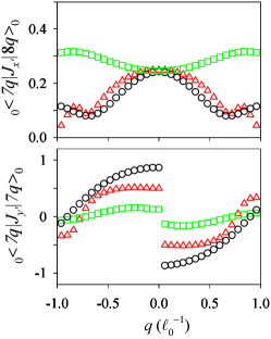
Figure 5: (Color online) Wavenumber dependence of the matrix elements entering Eq. (15) and (16) for $I=7$. Circles, triangles and squares are for increasing values of the Rashba intensity ${\cal R}_{z^{\prime}}=0.1\hbar\omega_{0}\ell_{0}$, $1.5\hbar\omega_{0}\ell_{0}$ and $2.6\hbar\omega_{0}\ell_{0}$, respectively. (Other parameters: $a=150$, $B=0$.)

IV.2 Perpendicular field

For ${\cal H}^{(Z)}\propto J_{y^{\prime}}$ the band maxima are shifted in opposite directions for positive and negative $q$’s (Fig. 1 right panel). This implies that the energy difference determining the g factor corresponds now to states with opposite wavenumbers, say $q_{m}$ and $-q_{m}$. For nonzero $q_{m}$ the two states $\varepsilon_{I0}(q_{m})$ and $\varepsilon_{(I+1)0}(q_{m})$ are nondegenerate and, for a sufficiently small field, we should have $\delta<<\varepsilon_{I}(q_{m}),\gamma_{I}$ in Eq. (13). As a matter of fact, we find that $\delta$ actually vanishes for the perpendicular field. This is the regime of non-degenerate first-order perturbation theory with modified energies $\varepsilon_{I0}(q_{m})+\gamma_{I}$ and $\varepsilon_{(I+1)0}(q_{m})+\gamma_{I+1}$. With the explicit definition of the $\gamma$’s and noting that $\varepsilon_{I0}(q_{m})=\varepsilon_{I0}(-q_{m})$ and $\gamma_{I}(q)=-\gamma_{I}(-q)$ for any $q$ (Fig. 5) the perpendicular g factor reads

$$g_{\perp}^{(I)}=\frac{4}{3}\kappa\left|\rule{0.0pt}{11.38092pt}\,_{0}\!\langle Iq_{m}|J_{y^{\prime}}|Iq_{m}\rangle_{0}\right|\;.$$ (16)

It seems natural that in $y^{\prime}$ orientation the g factor is simply proportional to the expectation value of $J_{y^{\prime}}$. Figure 5 shows the variation of this expectation value with the wavenumber and the Rashba intensity. Notice that typically $-0.5<q_{m}<0.5$, i.e., the maxima are located in the central part of Fig. 5 lower panel. When the Rashba intensity ${\cal R}_{z^{\prime}}$ increases there is a severe reduction of $\langle J_{y^{\prime}}\rangle_{0}$ in absolute value for this central region. This is the mechanism by which the Rashba interaction quenches the transverse g factor; namely, by means of a strong reduction of the transverse $y^{\prime}$ spin component.

For strong spin-orbit coupling the expectation values of all three components of the spin vector at zero magnetic field, $\langle\vec{J}\rangle_{0}$, vanish; a manifestation of the spin randomization induced by the Rashba field $\vec{\cal R}$. In $y^{\prime}$ orientation this induces a quenching of the g factor through Eq. (16) but, quite remarkably, Kramers degeneracy at zero wavenumber keeps the parallel g factor almost unaffected by virtue of the transition matrix elements in Eq. (15).

The g factors obtained from Eqs. (15) and (16) nicely agree with the results from the full diagonalization when orbital effects of the magnetic field are also neglected in the latter. The comparison with the complete model, results of Fig. 3, is less good; the trends are qualitatively reproduced but differences may be as large as a factor two. Orbital effects of the field are thus quite important for a precise analysis.

V Conclusion

We have attributed the anisotropy of magnetotransport g factors in hole quantum wires to the Rashba interaction. When the wire deformation and Rashba interaction are both large enough ($a>100$, ${\cal R}_{z^{\prime}}>2.5\hbar\omega_{0}\ell_{0}$) $g_{\perp}^{(N)}$ is greatly quenched by the Rashba interaction and $g_{\parallel}^{(N)}$ is almost unaffected. For lower wire deformations ($a<100$) we find a fluctuating, sample dependent behavior of the g factors.

Appendix A Field along $z^{\prime}$

Experimental g factors are usually obtained for magnetic fields in the $x^{\prime}y^{\prime}$ plane, either in parallel ($x^{\prime}$) or perpendicular ($y^{\prime}$) direction with respect to the wire. For completeness, in this Appendix we discuss in a qualitative way the effects of the magnetic field when this points along the growth direction $z^{\prime}$. The energy bands are similar to those of the $x^{\prime}$ orientation (middle panel of Fig. 1): they are symmetric respect to $q$-inversion, with anticrossing points at $q=0$, although the $B$-induced splitting is much stronger. This enhancement agrees with experimentsdan97 and is surely due to the important orbital motions induced by the field in this geometry. We thus obtain $g_{z^{\prime}}>g_{\parallel}$, where $g_{z^{\prime}}$ and $g_{\parallel}$ denote the g factors for $z^{\prime}$ and $x^{\prime}$ fields, respectively.

Looking at the Rashba-field dependence, $g_{z^{\prime}}$ behaves similarly to $g_{\perp}$ (along $y^{\prime}$): it decreases with increasing $\mathcal{R}_{z^{\prime}}$ but does not vanish for the maximum value we have taken ($2.6\hbar\omega_{0}\ell_{0}$). For strong wire deformation the saturation value corresponds to $g_{z^{\prime}}\approx 5$, while for in-plane magnetic field it corresponds to $g_{\parallel,\perp}\approx 1.5$ (see Fig. 3). For small values of $a$ the behavior of $g_{z^{\prime}}$ is less regular, as for the other orientations, but it tends to increase with $a$. Within the two-band model of Sec. IV we expect

$$g_{z^{\prime}}^{(I)}=\frac{4}{3}\kappa\bigg{|}\,_{0}\langle I0|J_{z^{\prime}}|(I+1)0\rangle_{0}\bigg{|}\;,$$ (17)

which is equivalent to Eq. (15), replacing $J_{x^{\prime}}\rightarrow J_{z^{\prime}}$, and is now depending on the value of the Rashba intensity.

Appendix B basis truncation

This Appendix discusses the relevance of the truncation of the number of oscillator states for the $y^{\prime}$ and $z^{\prime}$ oscillators. It is usually assumed that the confinement allows the truncation to the lowest, or few lowest, states. Here we explicitly check this quantitatively for selected values of $a$, the ratio of the two confinement strengths. We restrict, for simplicity, to the $B=0$ case with strong Rashba coupling in the growth direction.

Figure 6 displays the evolution of the band structure when a) increasing $N_{y^{\prime}}$ and $N_{z^{\prime}}$ sequentially from left to right panels; and b) increasing the deformation degree $a$ from top to bottom panels. The right column shows results that are very close to physical convergence. Looking at the successive band crossings at $q=0$, we notice that the truncation to $(N_{y^{\prime}},N_{z^{\prime}})=(1,1)$ grossly overestimates the energy separation between pairs of bands in all cases. It is remarkable that for increasing flatness degree the $(1,1)$ truncation deviates more and more from the right column. This is a consequence of the intersubband couplings induced by the kp and Rashba Hamiltonians: at least a few bands in the shallow oscillator ($y^{\prime}$) are essential even for large $a$’s.

More reasonable results are found for $(N_{y^{\prime}},N_{z^{\prime}})=(10,1)$, although the differences with the $(10,10)$ basis are still large quantitatively. In this case, however, increasing $a$ improves the quality of the description since intersubband coupling is allowed at least in $y^{\prime}$ direction. Finally, the $(10,2)$ results are close to the converged ones and only the insets reveal that sizeable differences are present at intermediate or low values of $a$. These differences are small in the behavior of the upper bands and become more and more important as the energy is reduced. From this analysis we conclude that for our present purpose, namely the description of magneto-g-factors of several successive conductance steps, it is essential to include enough oscillator bands in both $y^{\prime}$ and $z^{\prime}$ oscillators.

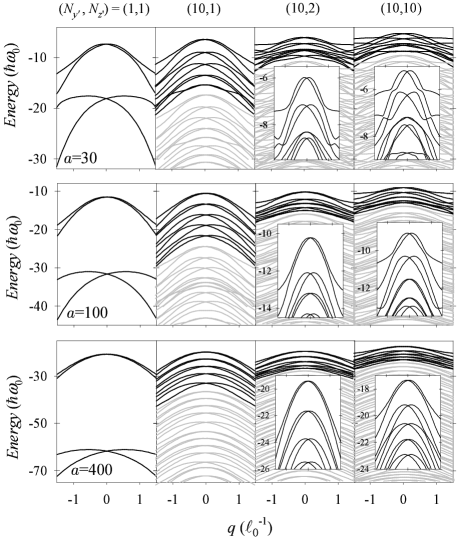
Figure 6: Evolution of the energy bands for selected numbers $(N_{y^{\prime}},N_{z^{\prime}})$ of oscillator states in the matrix discretization (columns) and aspect ratios $a$ (rows). The gray colour results are qualitative, indicating that the corresponding energy regions are full of bands. The insets in the rightmost columns show the details of those dense band distributions. Parameters: $B=0$, ${\cal R}_{z^{\prime}}=2.6\hbar\omega_{0}\ell_{0}$, ${\cal R}_{y^{\prime}}=0$, growth direction $(001)$ and wire orientation $(110)$.

References

- (1) R. Winkler, Spin-orbit coupling effects in two-dimensional electron and hole systems Springer Tracts in Modern Physics (Springer-Verlag, Berlin, 2003).
- (2) A. J. Daneshvar, C. J. B. Ford, A. R. Hamilton, M. Y. Simmons, M. Pepper, and D. A. Ritchie, Phys. Rev. B 55, R13409 (1997).
- (3) R. Danneau, O. Klochan, W. R. Clarke, L. H. Ho, A. P. Micolich, M. Y. Simmons, A. R. Hamilton, M. Pepper, D. A. Ritchie, and U. Zülicke, Phys. Rev. Lett. 97, 026403 (2006).
- (4) S. P. Koduvayur, L. P. Rokhinson, D. C. Tsui, L. N. Pfeiffer, and K. W. West, Phys. Rev. Lett. 100, 126401 (2008).
- (5) O. Klochan, A. P. Micolich, L. H. Ho, A. R. Hamilton, K. Muraki, and Y. Hirayama, New J. Phys. 11, 043018 (2009); J. C. H. Chen, O. Klochan, A. P. Micolich, A. R. Hamilton, T. P. Martin, L. H. Ho, U. Zülicke, D. Reuter, and A D Wieck, New J. Phys. 12, 033043 (2010).
- (6) R. Winkler, S. J. Papadakis, E. P. de Poortere, and M. Shayegan, Phys. Rev. Lett. 85, 4574 (2000).
- (7) G. Goldoni, A. Fasolino, Phys. Rev. B 52 14118 (1995).
- (8) Y. Harada, T. Kita, O. Wada, and H. Ando Phys. Rev. B 74, 245323 (2006); Y. Harada, T. Kita, O. Wada, H. Ando, and H. Mariette, Phys. Rev. B 78, 073304 (2008).
- (9) D. Csontos and U. Zülicke, Phys. Rev. B 76, 073313 (2007); D. Csontos and U. Zülicke, P. Brusheim, and H. Q. Xu, Phys. Rev. B 78, 033307 (2008); D. Csontos and U. Zülicke, App. Phys. Lett. 92, 023108 (2008); D. Csontos, P. Brusheim, U. Zülicke, and H. Q. Xu, Phys. Rev. B 79, 155323 (2009).
- (10) C. H. L. Quay, T. L. Hughes, J. A. Sulpizio, L. N. Pfeiffer, K.W. Baldwin, K.W. West, D. Goldhaber-Gordon and R. de Picciotto, Nature Phys. 6, 336 (2010).
- (11) S. Chesi, G. F. Giuliani, L. P. Rokhinson, L. N. Pfeiffer, and K. W. West, Phys. Rev. Lett. 106, 236601 (2011).
- (12) J. Pingenot, C. E. Pryor, M. E. Flatté, preprint (arxiv:10 11.5014v1).
- (13) L. Serra, D. Sánchez, R. López, Phys. Rev. B 72, 235309 (2005).