Universal and non-universal amplitude ratios for scaling corrections on Ising strips

Abstract

We consider strips of Ising spins at criticality. For strips of width $N$ sites, subdominant (additive) finite-size corrections to scaling are assumed to be of the form $a_{k}/N^{k}$ for the free energy, and $b_{k}/N^{k}$ for inverse correlation length, with integer values of $k$. We investigate the set $\{a_{k},b_{k}\}$ ($k\geq 2$) by exact evaluation and numerical transfer-matrix diagonalization techniques, and their changes upon varying anisotropy of couplings, spin quantum number $S$, and (finite) interaction range, in all cases for both periodic (PBC) and free (FBC) boundary conditions across the strip. We find that the coefficient ratios $b_{k}/a_{k}$ remain constant upon varying coupling anisotropy for $S=1/2$ and first-neighbor couplings, for both PBC and FBC (albeit at distinct values in either case). Such apparently universal behavior is not maintained upon changes in $S$ or interaction range.

I Introduction

In this paper we investigate corrections to scaling in critical Ising systems on a strip geometry. Consider a square lattice with $N$ lines and $M$ columns, in the limit $M\to\infty$. Other two-dimensional lattices, such as triangular or honeycomb, can be brought into a square-like shape, by suitable bond additions or deletions. From the largest ($\Lambda_{0}$) and second-largest ($\Lambda_{1}$) eigenvalues of the column-to-column transfer-matrix (TM), one obtains the free energy per spin, $f_{N}$ (in units of $k_{B}T$), and spin-spin correlation length $\xi_{N}$, via domb60 :

$$N\,f_{N}=\zeta\,\ln\Lambda_{0}\ ;\qquad\xi_{N}^{-1}=\zeta\,\ln\frac{\Lambda_{0}}{|\Lambda_{1}|}\ .$$ (1)

The factor $\zeta$ is unity for the square lattice and, in triangular and honeycomb geometries (also for the square lattice when the TM progresses along the diagonal baxter ; obpw96 ), corrects for the fact that the physical length added upon each application of the TM differs from one lattice spacing priv84 . In all cases of interest here, i.e., ferromagnetic systems, $\Lambda_{0}$ and $\Lambda_{1}$ are both real and positive.

At the critical point $T_{c}$ where a second-order transition takes place, conformal invariance cardy gives the following relations regarding universal quantities $c$, the conformal anomaly bcn86 , and the spin scaling dimension $x_{1}$ cardy84 :

$$\lim_{N\to\infty}N^{2}\,(f_{N}-f_{\infty})-2N\,f_{\rm surf}=\alpha\pi c\ ;$$ (2)

$$\lim_{N\to\infty}N\,\xi_{N}^{-1}=\beta\pi x_{1}\ .\qquad\qquad$$ (3)

In Eq. (2), where $c=1/2$ for models in the Ising universality class, $f_{\rm surf}=0$ for strips with periodic boundary conditions (PBC) across, and non-zero for free (FBC) or fixed BCs; $\alpha=\frac{1}{6}$ for PBC, and $\frac{1}{24}$ for FBC bcn86 . In Eq. (3), where the exponent $x_{1}$ for the Ising universality class is $x_{1}^{b}=\frac{1}{8}$ in the bulk, and $x_{1}^{s}=\frac{1}{2}$ for the ordinary surface transition, one has $x_{1}=x_{1}^{b}$, $\beta=2$ for PBC, and $x_{1}=x_{1}^{s}$, $\beta=1$ for FBC cardy84 .

Since Eqs. (2) and (3) are expected to be exact only asymptotically, it is of interest to develop a systematic understanding of the corresponding finite-$N$ corrections. We write:

$$N\,(f_{N}-f_{\infty})-2\,f_{\rm surf}=\sum_{k=1}^{\infty}\frac{a_{k}}{N^{k}}\ ,$$ (4)

$$\xi_{N}^{-1}=\sum_{k=1}^{\infty}\frac{b_{k}}{N^{k}}\ ,\qquad\qquad$$ (5)

where $a_{1}=\alpha\pi c$, $b_{1}=\beta\pi x_{1}$. Assuming only integer powers of $N^{-1}$ in Eqs. (4) and (5) is believed to be warranted as long as one is dealing with models in the Ising universality class cardy86 . We revisit this assumption in Sections IV and  V below. Our task here will be to learn as much as possible about the coefficients $\{a_{k},\,b_{k}\}$, $k\geq 2$, as well as (for reasons explained below) their ratios $b_{k}/a_{k}$. We are interested in their respective universality, or lack thereof, upon changes in boundary conditions, degree of spatial anisotropy of interactions, spin quantum number $S$, and (finite) interaction range. We restrict ourselves to the square lattice.

In Section II we investigate $S=1/2$ strips with PBC, first-neighbor interactions, and varying degrees of spatial anisotropy; in Sec. III, we examine systems with FBC, again with varying anisotropy; Sec. IV deals with the spin–$1$ case, and isotropic couplings only; in Sec. V we return to $S=1/2$ and introduce next-nearest-neighbor couplings (keeping to isotropic interactions). Finally, in Sec. VI, concluding remarks are made.

II Periodic boundary conditions

II.1 Preliminaries; isotropic systems

We recall results for strips cut along the $x$ direction, with $N$ lines and $M\to\infty$ columns, and PBC across. All eigenvalues of the TM can be written in closed form domb60 . With $K_{i}\equiv J_{i}/k_{B}T$ being the interactions respectively along $x$ ($i=1$) and $y$ ($i=2$), $\Lambda_{0}$ and $\Lambda_{1}$ are:

$$\ln\Lambda_{0}-\frac{1}{2}N\ln(2\sinh 2K_{1})=\frac{1}{2}\sum_{r=0}^{N-1}\gamma_{2r+1}\ ,\qquad\quad$$ (6)

$$\ln\Lambda_{1}-\frac{1}{2}N\ln(2\sinh 2K_{1})=\frac{1}{2}\sum_{r=0}^{N-1}\gamma_{2r}\ ,\qquad\qquad$$ (7)

where

$$\cosh\gamma_{r}=\cosh 2K_{1}^{\ast}\,\cosh 2K_{2}-\sinh 2K_{1}^{\ast}\,\sinh 2K_{2}\,\cos\omega_{r}\ ;$$ (8)

the dual couplings $K_{i}^{\ast}$ are defined by $\tanh K_{i}^{\ast}=\exp(-2K_{i})$, and the allowed frequencies are $\omega_{r}=r\pi/N$.

With $s_{i}\equiv\sinh 2K_{i}$, one has $s_{1}\,s_{2}=1$ at the critical temperature where the system is self-dual, and Eq. (8) becomes:

$$\cosh\gamma_{r}=1+\frac{1}{s_{1}^{2}}(1-\cos\omega_{r})\qquad(T=T_{c})\ .$$ (9)

For isotropic systems, $s_{1}=s_{2}=1$ at criticality. In this case, the sums in Eqs. (6) and (7) were tackled izhu01 by applying the extended Euler-MacLaurin summation formula abram ; ivizhu02 :

$$\sum_{n=0}^{N-1}F(a+nh+\alpha h)=\frac{1}{h}\int_{a}^{b}F(x)\,dx+\qquad\qquad\qquad$$

$$+\sum_{k=1}^{\infty}\frac{h^{k-1}}{k!}\,B_{k}(\alpha)\,\left(F^{(k-1)}(b)-F^{(k-1)}(a)\right)\ ,\qquad$$ (10)

where $h=(b-a)/N$, $F^{(j)}(x)$ is the $j$–th derivative of $F(x)$, $0<\alpha<1$, and the $B_{k}(\alpha)$ are the periodic Bernoulli polynomials (related to the Bernoullli numbers, denoted simply by $B_{k}$, by $B_{k}=B_{k}(0)$).

It was found that only odd powers of $N^{-1}$, i.e., $k=2j-1$, $j\geq 1$ occur in Eqs. (4) and (5); this can be traced back to the fact that the Bernoulli numbers $B_{m}$ obey $B_{2m-1}=0$ $(m>1)$. Also, relatively simple closed-form expressions were derived for all $a_{k}$ and $b_{k}$. Such expressions reproduce previously-known exact results (for $a_{1}$ bcn86 , $b_{1}$ cardy84 , and $b_{3}$ dds82 ), and are in very good agreement with numerically-obtained ones dq00 . Furthermore, although the coefficients themselves are non-universal (upon changing lattice structure, or considering quantum Ising chains pfeuty ; fs78 ; hb81 instead of their two-dimensional classical counterparts), their ratio is found to remain constant upon the same set of changes izhu01 :

$$\frac{b_{k}}{a_{k}}=\frac{2^{k+1}-1}{2^{k}-1}\quad(k=2j-1\ ,\ j\geq 1)\ [\,{\rm PBC}\,].$$ (11)

It should be noted that when one considers the TM running along the diagonal of the square lattice (as in Refs. baxter, ; obpw96, ), one gets for isotropic systems with PBC the same value for the ratio $b_{k}/a_{k}$ as in Eq. (11). Furthermore, the coefficients themselves have the same absolute value as those found with the TM along $x$; only, they alternate in sign: $a_{k}$, $b_{k}<0$ for $k=1$, positive for $k=2$ etc izpriv2 .

II.2 Anisotropic systems with PBC

With $K_{1}/K_{2}\equiv R\neq 1$, one gets inw86 ; nb83 the corresponding forms of Eqs. (2) and (3) [ specializing to Ising spins on strips with PBC ] as:

$$\lim_{N\to\infty}N^{2}\,(f_{N(i)}-f_{\infty})=\frac{1}{s_{i}}\,\frac{\pi}{12}\ ,$$ (12)

$$\lim_{N\to\infty}N\,[\,\xi_{N(1)}^{-1}\,\xi_{N(2)}^{-1}\,]^{1/2}=\frac{\pi}{4}\ ,$$ (13)

where $f_{N(i)}$ and $\xi_{N(i)}$ are, respectively, free energy and correlation length at criticality, both calculated by iterating the TM along the direction with couplings $K_{i}$. Note inw86 that $f_{\infty}$ in Eq. (12) also depends on $R$ . $s_{1}\equiv\sinh 2K_{c}$ is the solution of $\sinh 2K_{c}\,\sinh 2RK_{c}=1$.

As noted in Ref. izhu01, , Eq. (9) can be rewritten as:

$$\gamma(\omega)=2\,\ln(u+\sqrt{1+u^{2}})\ ,\qquad u\equiv\frac{1}{s_{1}}\sin\frac{\omega}{2}\ .$$ (14)

In this form, it is immediate to see that anisotropy brings about a simple rescaling of the argument in the sums of Eqs. (6) and (7). Furthermore, in the Euler-Maclaurin formula, $\gamma(\omega)$ only occurs through its derivatives of $n$-th order $\gamma^{(n)}$ at the endpoints $\omega=0$ and $\pi$, which satisfy $\gamma^{(n)}(\pi)=-\gamma^{(n)}(0)$, see Eq. (14). This is enough to guarantee that any coefficient $a_{k}(R)\ [\,b_{k}(R)]$ will differ from its isotropic counterpart $a_{k}(1)\ [\,b_{k}(1)]$ by a multiplicative correction, $g_{k}(s_{1})$. Thus, it is predicted in Ref. izhu01, that the ratios given in Eq. (11) will remain unchanged. In this context, Eqs. (12) and (13) reflect the (easily checkable) fact that $g_{1}(s_{1})=s_{1}^{-1}$, where for Eq. (13) one also uses $s_{1}\,s_{2}=1$ at criticality.

In order to test the robustness of the theoretical framework just expounded, we evaluated the third-order correction. This is done by replacing the argument of Eqs. (6) and (7) by its generalized form, Eq. (14), and following the corresponding effects on the $N^{-3}$ term in Eq. (10), which arise from the third-order derivatives indicated there. One finds:

$$g_{3}(s_{1})=\frac{1}{2s_{1}^{2}}(s_{1}+\frac{1}{s_{1}})=\frac{1}{2s_{1}t_{1}^{2}}\ ,$$ (15)

where $t_{1}\equiv\tanh 2K_{1}$.

We numerically calculated $f_{N}$ and $\xi_{N}^{-1}$ from Eqs. (1), (6), and (7) for assorted values of $R$, and $N=10j,\ j=2,3\dots 30$. The resulting sequences were adjusted to:

$$f_{N}(R)=f_{\infty}(R)+\frac{1}{s_{1}}\frac{\pi}{12N^{2}}+\frac{a_{3}(R)}{N^{4}}+\frac{a_{5}(R)}{N^{6}}\ ,$$ (16)

$$\xi_{N}^{-1}(R)=\frac{1}{s_{1}}\frac{\pi}{4N}+\frac{b_{3}(R)}{N^{3}}+\frac{b_{5}(R)}{N^{5}}\ ,\qquad\qquad\ \$$ (17)

where $f_{\infty}$, $\{a_{k}\}$, and $\{b_{k}\}$ are adjustable parameters. It is important to keep the next-higher-order terms $a_{5}$ and $b_{5}$ in the truncated expansions above, in order to improve stability for the quantities $a_{3}$ and $b_{3}$ which are the main focus of interest here. The optimum range of $N$, large enough for higher-order terms to have negligible influence, but not so large as to compromise the numerical accuracy of fits (since this depends crucially on differences between finite-$N$ estimates of $f_{N}$ and $\xi_{N}^{-1}$) was found to be $100\leq N\leq 300$. In Fig. 1 we show $a_{3}(R)$ and $b_{3}(R)$, fitted via Eqs. (16) and (17), for several values of $R$ spanning four orders of magnitude. The continuous lines depict Eq. (15), multiplied respectively by the isotropic values $a_{3}(1)=7\pi^{3}/1440$, $b_{3}(1)=\pi^{3}/96$ dds82 ; dq00 ; izhu01 . The agreement is perfect, except for $a_{3}(R)$ at $R\gtrsim 30$ where reasonable convergence was only obtained upon adding the next higher-order term, $a_{7}(R)/N^{8}$, in Eq. (16).

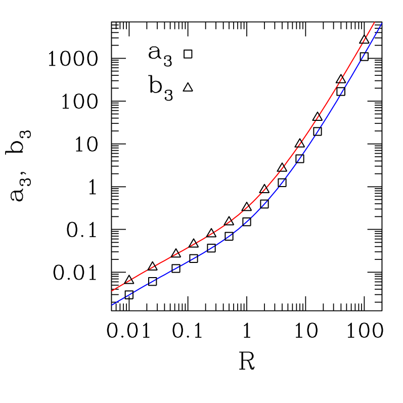
Figure 1: (Color online) Points: results for $a_{3}(R)$, $b_{3}(R)$ defined in Eqs. (16) and  (17), from fits of $f_{N}$, $\xi_{N}^{-1}$ data evaluated for strips of widths $100\leq N\leq 300$ and PBC across, via Eqs. (1), (6), and (7). Uncertainties are smaller than symbol sizes. Full lines show $g_{3}(s_{1})$ defined in Eq. (15), multiplied respectively by $a_{3}(1)$ [blue] and $b_{3}(1)$ [red] (see text).

Our results provide direct numerical evidence that the Euler-Maclaurin scheme used in Ref. izhu01, is indeed applicable to Ising systems with PBC and any finite degree of (ferromagnetic) anisotropy. Similar conclusions were drawn for the anisotropic Ising model with Braskamp-Kunz boundary conditions izyeh09 .

It is interesting to consider the above results for $R\leavevmode\nobreak\ \to\leavevmode\nobreak\ \infty$. It is known fs78 ; hb81 ; bg85 ; mh87 that the [zero-temperature] quantum Ising chain (QIC) in a transverse field pfeuty has a correspondence with this extreme anisotropic limit, via: $f_{\infty}\leftrightarrow E_{0}$, $\xi^{-1}\leftrightarrow E_{1}-E_{0}$ etc, where the $E_{i}$ are the energy levels of the quantum system. In Ref. izhu01, the energy spectrum of the QIC with PBC was studied directly with help of the Euler-Maclaurin formula, and the corresponding ratio $b_{k}/a_{k}$ was found to obey Eq. (11). The latter result can also be extracted from the exact expressions Eqs. (17a) and (18a) of Ref. bg85, .

While the limit given in Eq. (13) is preserved as $R\to\infty$, the exponential divergence of the higher-order terms is not cancelled:

$$[\,\xi_{N(1)}^{-1}\,\xi_{N(2)}^{-1}\,]^{1/2}=\frac{\pi}{4N}+\frac{1}{4}\,(s_{1}+\frac{1}{s_{1}})^{2}\,\frac{\pi^{3}}{96N^{3}}+\cdots\ .$$ (18)

A similar effect (with the factor $1/s_{1}$) is already obvious in Eq. (12). In summary, although coefficient ratios $b_{k}/a_{k}$ are preserved as $R\to\infty$, each term of the Euler-Maclaurin expansion for the two-dimensional Ising model with $R\gg 1$ is translated into its counterpart of the corresponding expansion for the QIC by means of a distinct anisotropy factor.

III Free boundary conditions

III.1 Isotropic systems

The eigenvalue spectrum of the TM has been obtained dba71 ; aks88 ; aks89 for Ising $S=1/2$ strips with nearest-neighbor couplings and free boundary conditions (FBC) across. For a strip of width $N$ sites, one has:

$$\ln\Lambda_{m}=\frac{1}{2}\sum_{i=1}^{N}\pm\gamma(\omega_{i})\ ,\quad m=0,\cdots,2^{N}-1,$$ (19)

where the $\pm$ combinations run through all $2^{N}$ possibilities. A regular background term, $\frac{1}{2}N\ln(2\sinh 2K_{1})$ [ see Eqs. (6) and (7) ], has been omitted. With all the $\gamma(\omega_{i})$ real and positive for this case dba71 ,

$$\ln\Lambda_{0}=\frac{1}{2}\sum_{n=1}^{N}\gamma(\omega_{n})\ ;$$ (20)

$$\xi_{N}^{-1}=\gamma(\omega_{1})\ ,\qquad\quad$$ (21)

where $\omega_{1}$ corresponds to the smallest $\gamma$. The relationship between the $\gamma$ and the allowed frequencies $\omega_{i}$ is given by dba71 :

$$\cosh\gamma=\cosh 2K_{1}^{\ast}\,\cosh 2K_{2}-\sinh 2K_{1}^{\ast}\,\sinh 2K_{2}\,\cos\omega\ ;\ \\$$ (22)

$$\sinh\gamma\,\cos\delta^{\ast}=\sinh 2K_{2}\,\cosh 2K_{1}^{\ast}-$$

$$-\cosh 2K_{2}\,\sinh 2K_{1}^{\ast}\,\cos\omega\ ;\$$ (23)

$$\sin\omega/\sinh\gamma=\sin\delta^{\ast}/\sinh 2K_{1}^{\ast}\ .\qquad\qquad$$ (24)

From Eqs. (22), (23), and  (24), one gets at the critical point, where $s_{1}\,s_{2}=1$:

$$\cosh\gamma=1+\frac{1}{s_{1}^{2}}(1-\cos\omega)\ ;\qquad\qquad\$$ (25)

$$\tan\delta^{\ast}=t_{1}\,\frac{\sin\omega}{(1-\cos\omega)}\ ,\qquad\quad$$ (26)

again with $t_{1}\equiv\tanh 2K_{1}$. From Eq. (25), the smallest $\gamma$ corresponds to the lowest allowed $\omega$. Note also that Eq. (25) is identical in form to Eq. (9), so it can also be rewritten as Eq. (14). Finally, the allowed frequencies $\omega_{n}$ can be determined from Eq. (26) combined with the quantization condition dba71 :

$$e^{i\,N\,\omega}=\pm e^{i\,\delta^{\ast}}\ ,\quad 0\leq\omega\leq\pi\ ,$$ (27)

by eliminating the auxiliary angle $\delta^{\ast}$.

For the remainder of this Subsection, we shall consider only isotropic systems ($K_{1}=K_{2}$), thus $s_{1}=1$, $t_{1}=1/\sqrt{2}$ in Eqs. (25) and (26).

The resulting frequencies are not equally spaced, as illustrated in Fig. 2. So the Euler-Maclaurin formula cannot be used in the same way as in Ref. izhu01, , to calculate the free energy from Eq. (20). However, we show in the following that one can still make adaptations and extract some useful information.

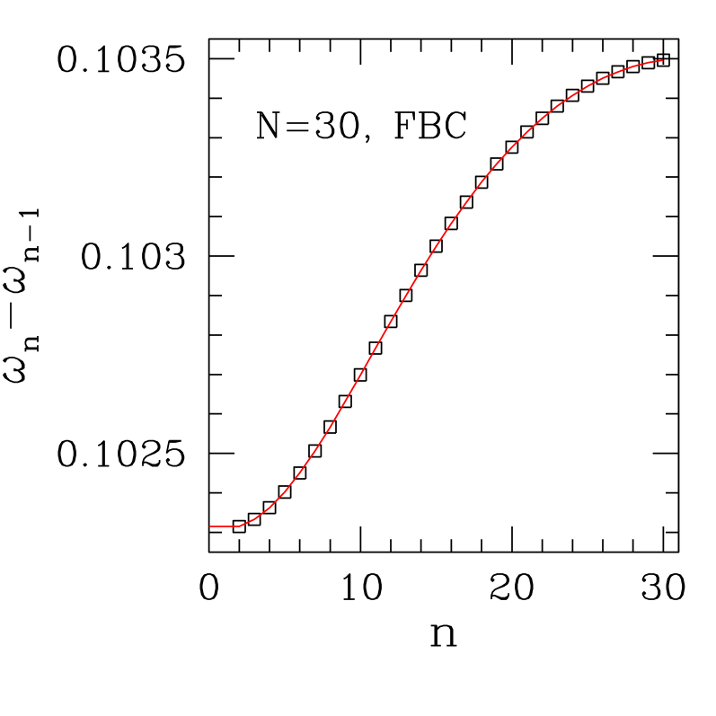
Figure 2: (Color online) Ising strips with FBC and isotropic interactions, at $T_{c}$: differences $\omega_{n}-\omega_{n-1}$ ($n\geq 2$) between consecutive solutions of Eqs. (26) and (27), for strip of width $N=30$ sites.

We found that for large $N$ the $\omega_{n}$ approach the form:

$$\omega_{n}=\omega_{n}^{0}+\frac{1}{N}\,f\left(\frac{n}{N}\right),\quad\omega_{n}^{0}\equiv\left(n-\frac{1}{2}\right)\frac{\pi}{N}\ ,\ 1\leq n\leq N\ .$$ (28)

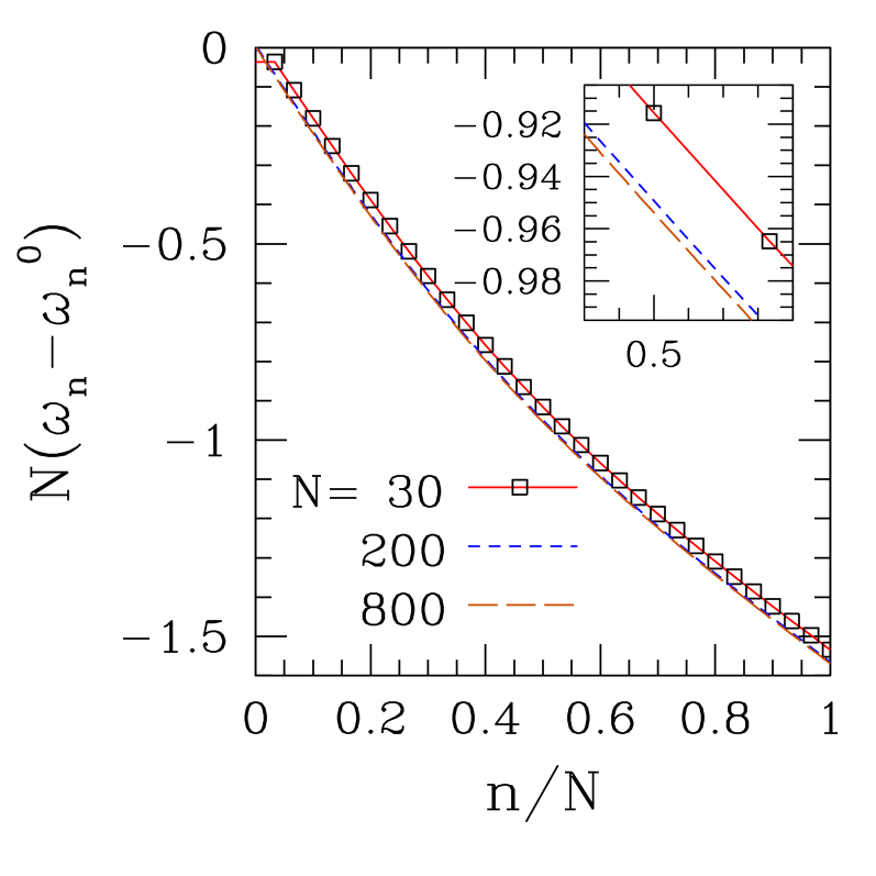
Figure 3: (Color online) Ising strips with FBC and isotropic interactions, at $T_{c}$: illustrating the convergence of $N(\omega_{n}-\omega_{n}^{0})$ towards $f(n/N)$ with increasing $N$; see Eq. (28). The inset is a blowup of the central section of the main figure.

As shown in Fig. 3, $f(u)$ is a smoothly varying function of $u=n/N$. One has: $f(0)=0$, $\lim_{\,u\to 1}f(u)=-\pi/2$. Both limits can be understood by examination of the graphical solutions of Eqs. (26) and (27) aks89 . The residual $N$-dependence of $N(\omega_{n}-\omega_{n}^{0})$ is highlighted in the inset of Fig. 3. This can be accounted for by an additive correction of the form $(1/N)\,f_{2}(n/N)$; $f_{2}$ is nearly constant, varying smoothly between $\approx 1.1$ and $1.3$ for $0<n/N<1$. We thus write:

$$\gamma(\omega_{n})=\gamma(\omega_{n}^{0})+\sum_{j=1}^{\infty}\frac{1}{N^{j}}\,g^{(j)}(\omega_{n}^{0})\ ,$$ (29)

with

$$g^{(1)}(\omega_{n}^{0})\equiv\left\{f(\omega)\,\gamma^{(1)}(\omega)\right\}_{\omega_{n}^{0}}\ ,\qquad\qquad$$

$$g^{(2)}(\omega_{n}^{0})\equiv\left\{f_{2}(\omega)\,\gamma^{(1)}(\omega)+\frac{1}{2!}\,f^{2}(\omega)\,\gamma^{(2)}(\omega)\right\}_{\omega_{n}^{0}}\ \dots\qquad$$ (30)

where $\gamma^{(m)}\equiv d^{m}\gamma/d\omega^{m}$, and the arguments of $f$ and $f_{2}$ have been straightforwardly changed. Eq. (20) then becomes:

$$\ln\Lambda_{0}=\frac{1}{2}\sum_{n=1}^{N}\gamma(\omega_{n}^{0})+\frac{1}{2N}\sum_{n=1}^{N}g^{(1)}(\omega_{n}^{0})+\dots\equiv\sum_{j=0}^{\infty}S_{j}\ ,$$ (31)

So, each term (of order $j\geq 0$, with $g^{(0)}(\omega_{n}^{0})\equiv\gamma(\omega_{n}^{0})$) of the Taylor expansion indicated in Eq. (29) gives rise to a sum $S_{j}$ of $N$ terms, each of the latter evaluated at $\omega=\omega_{n}^{0}$ ($1\leq n\leq N$), i.e., at equally spaced intervals.

We investigated the feasibility of applying the Euler-Maclaurin formula, Eq. (10), to each $S_{j}$, with $x=\omega$, $h=\pi/N$, $a=0$, $b=\pi$, $\alpha=1/2$, so that the result would be of the form $S_{j}=\sum_{i=-1}^{\infty}a_{i}^{j}/N^{(i+j)}$ [ where $i=-1$ corresponds to the integral in Eq. (10) ]. $S_{j}$ would then give contributions to $\ln\Lambda_{0}$ at all orders $N^{-(j+i)}$, $i\geq-1$. Note that $a_{0}^{j}\equiv 0$ because $B_{1}(1/2)$=0 abram ; ivizhu02 . However, one would have to assume that the infinite sum implicit in each Taylor series commutes with the infinite sum present in each separate Euler-Maclaurin expansion (the form given in Eq.(10) assumes that the remainder term vanishes; see, e.g., Ref. ivizhu02, ). Having in mind that the expansion parameter of the Taylor series and the sampling interval of the Euler-Maclaurin formula can be of the same order ($\pi/N$), it is doubtful that such commutation can be guaranteed.

With these words of caution in mind, here we evaluate only a few of the lowest-order terms which would occur in such a calculational framework.

We applied the Euler-Maclaurin formula to $S_{0}$ in Eq. (31). This differs from the sum indicated in its PBC counterpart, Eq. (6), in that the frequency spacing here is half that in the latter Equation. For the corresponding integral of Eq. (10), this is compensated by the fact that the integration interval is cut in half as well, so from $a_{-1}^{0}$ one reobtains the bulk result $f_{\infty}-(1/2)\ln 2=(2G/\pi)$, $G=0.915965594\dots$ (Catalan’s constant) domb60 . For the terms of Eq. (10) involving derivatives of the $m$–th order, the corresponding term in $S_{0}$ has an extra factor $2^{-(1+m)}$ relative to its PBC analogue izhu01 . One gets $a_{1}^{0}=\pi/48$ as given by conformal invariance bcn86 , $a_{3}^{0}=0.00942\dots$ izhu01 .

For $S_{1}$, we evaluated $I\equiv\int_{0}^{\pi}g^{(1)}(\omega)\,d\omega$ using finite-$N$ approximations for $f(x)$ with $200\leq N\leq 2000$, and extrapolating the resulting sequence against $1/N$. The final result is $I/2\pi=a_{-1}^{1}=-0.1817309(1)$, to be compared with $2f_{\rm surf}=-0.18173148\dots$ au-yang . In the computation of higher-order terms, we ran into inconsistencies between results thus obtained, and those coming from direct numerical evaluation of the free energy via Eq. (20). We conjecture that these difficulties stem from the conceptual problems in interchanging the order of infinite sums, referred to above.

As regards the correlation length, from Eq. (21) above, and combining Eqs. (3) and (14), one has for the finite-$N$ estimate $\eta_{1}^{s}(N)$ of the decay-of-correlations exponent $\eta_{1}^{s}=2x_{1}^{s}$:

$$\eta_{1}^{s}(N)=\frac{2N}{\pi}\ln\,[y+\sqrt{y^{2}+1}]\ ,\quad y=2-\cos\omega_{1}\ .$$ (32)

By solving Eqs. (26) and (27) in the limit $\omega\to 0$, $\delta^{\ast}\to\pi/2$, and consequently taking $y\to 1$ in Eq. (32), one gets:

$$\eta_{1}^{s}(N)=1-\frac{1}{\sqrt{2}}\,\frac{1}{N}+\left[\frac{1}{2}-\frac{\pi^{2}}{48}\right]\,\frac{1}{N^{2}}+{\cal O}(N^{-3})\ .$$ (33)

According to Eq. (33), both odd and even powers of $N^{-1}$ are predicted to arise in the expansion of $\xi_{N}^{-1}$ for this case. For Ising systems with FBC, the occurrence of $N^{-1}$ corrections to finite-$N$ estimates of scaling powers was noted in Ref. bg85b, .

We evaluated $f_{N}$ and $\xi_{N}$ for $N=10j$, $j=2,\dots,30$, by numerically solving for the allowed frequencies and then plugging the results into Eq. (25) and, finally, Eq. (19).

We fitted free-energy data for $100\leq N\leq 300$ to a truncated form of Eq. (4), with $k\leq 4$. After ensuring that known quantities were reproduced to good accuracy when allowed to vary freely, we fixed them at their known values, namely $f_{\infty}=(1/2)\ln 2+(2G/\pi)$ domb60 ; $f_{\rm surf}=-0.0908657\dots$ au-yang ; $a_{1}=\pi/48$, with the results: $a_{2}=-0.04616(2)$, $a_{3}=0.024(1)$, $a_{4}=0.69(6)$. Note that $a_{3}$ as given here differs from $a_{3}^{0}$ evaluated from $S_{0}$ above, in connection with Eq. (31). This is because $a_{3}$ gets additional contributions from higher-order sums $S_{k}$, $k>0$ (not calculated there).

A fit of a subset ($100\leq N\leq 300$) of the $\eta_{1}^{s}(N)$ thus obtained to the form $\eta_{1}^{s}(N)=\eta_{1}^{s}+\sum_{k=1}^{4}b^{\,\prime}_{k}\,N^{-k}$ gave $\eta_{1}^{s}=1\ (\pm 1\times 10^{-10})$, $b_{1}^{\,\prime}=-0.70710680(3)$, $b_{2}^{\,\prime}=0.294388(7)$, $b_{3}^{\,\prime}=0.2274(7)$, $b_{4}^{\,\prime}=-0.68(3)$. By keeping $\eta_{1}^{s}$, $b_{1}^{\,\prime}$, $b_{2}^{\,\prime}$ fixed at the respective values predicted in Eq. (33), we obtained $b_{3}^{\,\prime}=0.227972(6)$, $b_{4}^{\,\prime}=-0.7013(6)$. The above results both confirm the predictions of Eq. (33) for $b_{1}^{\,\prime}$ and $b_{2}^{\,\prime}$, and indicate that, in general, both even and odd powers of $N^{-1}$ occur in the expansion whose lowest-order terms are given in that Equation.

We defer analysis of the ratios $b_{k}/a_{k}$ thus obtained until the next Subsection, where anisotropic systems with FBC, and their connection to the QIC with free ends, are discussed.

III.2 Anisotropic systems with FBC

We first note that, even though Eq. (14) is valid here, the arguments given immediately below it do not seem to cover the present case, since for FBC the $\omega_{n}$ depend on anisotropy in the non-trivial way given in Eqs. (26) and  (27). Thus it is not obvious whether, e.g., Eq. (15) still applies to the free energy here.

We have directly examined the $\omega_{n}$, for varying anisotropies, and seen that their behavior is qualitatively similar to that for the isotropic case, depicted in Figs. 2 and 3. In particular, the limits $f(0)=0$ and $f(1)=-\pi/2$ still hold [ see the comments following Eq. (28) ].

By incorporating anisotropy into Eq. (32) via Eq. (14), one gets the generalized version of Eq. (33):

$$\eta_{1}^{s}(N)=\frac{1}{s_{1}}\left\{1-\frac{1}{2t_{1}}\frac{1}{N}+\frac{1}{2t_{1}^{\,2}}\left[\frac{1}{2}-\frac{\pi^{2}}{48}\right]\frac{1}{N^{2}}\right\}+\cdots\ .$$ (34)

We numerically calculated $f_{N}$ and $\xi_{N}^{-1}$ from Eqs. (1), (20), and (21) for assorted values of $R$, and $N=10j,\ j=2,3\dots 30$. Bearing in mind the FBC-adapted forms of Eqs. (12) and (13) inw86 ; nb83 , the resulting sequences were adjusted to:

$$N(f_{N}-f_{\infty})=2f_{\rm surf}+\frac{1}{s_{1}}\frac{\pi}{48N}+\sum_{k=2}^{4}\frac{a_{k}(R)}{N^{k}}\ ,\qquad$$ (35)

$$\xi_{N}^{-1}(R)=\frac{1}{s_{1}}\frac{\pi}{2N}+\sum_{k=2}^{4}\frac{b_{k}(R)}{N^{k}}\ ,\qquad\qquad$$ (36)

where $f_{\infty}$, $f_{\rm surf}$ (both of which, as well as $f_{N}$, also depend on $R$), $\{a_{k}\}$, and $\{b_{k}\}$ are adjustable parameters. The $b^{\prime}_{k}$, defined in connection with Eqs. (32) and (33), relate to the $b_{k}$ of Eq. (36) by $b_{k}=(\pi/2)\,b_{k-1}^{\prime}$. As done in Section II, we keep the next-higher-order terms $a_{4}$ and $b_{4}$ in the truncated expansions above, in order to improve stability for the quantities $a_{2}$, $a_{3}$, $b_{2}$, and $b_{3}$ which are the main focus of interest here. Similarly, the range of $N$ used in our fits was $100\leq N\leq 300$. In Fig. 4 we show $a_{2}(R)$, $a_{3}(R)$, $b_{2}(R)$, and $b_{3}(R)$, fitted via Eqs. (35) and (36), for several values of $R$ spanning four orders of magnitude. The lines depict the anisotropy factors from Eq. (34), namely $g_{2}\equiv(2s_{1}t_{1})^{-1}$ (dashed) and $g_{3}\equiv(2s_{1}t_{1}^{2})^{-1}$ (full) multiplied by the pertinent values of $a_{2}(1)$ and $b_{2}(1)$ [ for $g_{2}\,$] or $a_{3}(1)$ and $b_{3}(1)$[ for $g_{3}\,$]. Once again, the agreement is perfect. The only case for which the higher-order terms ($a_{4}$ or $b_{4}$) made any perceptible difference was for $a_{3}(R)$ at $R\gtrsim 30$.

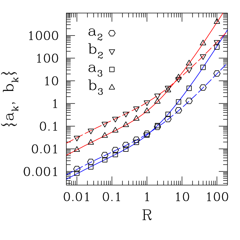
Figure 4: (Color online) Points: results for $\{a_{k}(R)$, $b_{k}(R)\,\}$ defined in Eqs. (35) and (36) [ absolute values for $k=2\,$], from fits of $f_{N}$, $\xi_{N}^{-1}$ data evaluated for strips of widths $100\leq N\leq 300$ and FBC across. Uncertainties are smaller than symbol sizes. Lines show anisotropy factors defined in Eq. (34), multiplied respectively by $a_{k}(1)$ [blue] and $b_{k}(1)$ [red] [$k=2,3$] (see text).

Our results provide direct numerical evidence that the coefficient ratios $b_{2}/a_{2}=24.06(2)$ and $b_{3}/a_{3}=19.3(6)$ remain constant against any finite degree of (ferromagnetic) anisotropy. Note that $b_{3}/a_{3}$ differs substantially from the PBC value $15/7$ izhu01 . It is remarkable that the free-energy coefficients depend on anisotropy in the same way as those for the correlation length. As stated in the first paragraph of this Section, this is not obviously granted at the outset.

We consider the extreme anisotropic limit $R\to\infty$ of Ising strips with FBC, and its connection to the QIC with FBC at both ends pfeuty ; bg85 . In Ref. izhu09, , the exact expressions for ground-state energy and energy gaps of the QIC, given in Ref. pfeuty, , were written as Euler-Maclaurin expansions; similarly to the PBC case, only odd powers of $N^{-1}$ were found to occur in the corresponding forms of Eqs. (4) and (5). The counterpart to Eq. (11) in this case was shown to be:

$$\frac{b_{k}}{a_{k}}=\frac{2(k+1)}{(2^{k}-1)\,B_{k+1}}\quad(k=2j-1\ ,\ j\geq 1)\ [\,{\rm FBC}\,]\leavevmode\nobreak\ .$$ (37)

For $k=1$, this agrees with the conformal-invariance results of Eqs. (2) and (3); for $k=3$, Eq. (37) gives $b_{3}/a_{3}=-240/7$ izhu09 .

Our results above for classical Ising spins differ from those for the QIC in that: (i) both even and odd powers of $N^{-1}$ occur, in free-energy as well as in correlation-length expansions; and (ii) $b_{3}/a_{3}=+19.3(6)$, incompatible with the value given in Ref. izhu09, .

Note however that, when one considers the two-dimensional classical Ising model with the TM running along the diagonal obpw96 , in the corresponding version of FBC, a picture closer to that found for PBC emerges, namely izpriv : only odd powers of $N^{-1}$ occur in Eqs. (4) and  (5), and the value $b_{3}/a_{3}=-240/7$ is reproduced.

IV S=1

We considered $S=1$ Ising systems on a square lattice, with both PBC and FBC, and isotropic couplings only. The critical temperature is known rather accurately bcg03 , $J/k_{B}T_{c}=K_{c}=0.590473(5)$.

In this case, no closed-form expressions for the TM eigenvalues are forthcoming, so one must rely on numerical diagonalization. The first consequence of this fact is that the assumption of only integer powers in Eqs. (4) and (5) must be reanalyzed. Indeed, while in Sections II and III one could verify directly from the respective closed-form equations that no noninteger powers of $N^{-1}$ were allowed, here this possibility does not arise. Furthermore, it has been shown for models very closely related to the standard Ising model that fractional powers occur in corrections to scaling bf85 ; bdn88 . It was conjectured that these would take the form $N^{-4/3}$, clearly a very important term in the current context. However, for the $S=1$ Ising model on a square lattice, it has been numerically shown that the amplitude of a hypothetical $N^{-4/3}$ term is most likely zero bdn88 , so in the current Section at least, one can retain Eqs. (4) and (5) in their original form.

Secondly, the range of strip widths within practical reach is much restricted in comparison with $S=1/2$ systems. We used $4\leq N\leq 16$. Such a narrow range was, by far, the most quantitatively relevant source of systematic inaccuracies in our estimates of corrections to scaling, far outweighing, e.g., the uncertainties in $T_{c}$.

In order to assess the associated effects, we produced fits of free-energy and correlation-length data for sets of $S=1/2$ data restricted to the same range of $N$. For PBC, we took truncated forms of Eqs. (4) and (5) using the exact values of $f_{\infty}$, $a_{1}$, and $b_{1}$, with $\{a_{k},b_{k}\}$ as adjustable parameters for $k=3,5,7$, and zero otherwise. The $k=7$ terms were included in order to increase stability for the $k=3$ and $5$ ones. By further restricting the range of data fitted to $10\leq N\leq 16$, we found very good agreement with the known values dq00 ; izhu01 of $a_{3}$, $b_{3}$, while for $a_{5}$ and $b_{5}$ deviations were of order $5\%$ (see Table 1).

Turning to $S=1$ with PBC, allowing for $a_{2}$, $b_{2}\neq 0$ in Eqs. (4) and (5) gave fitted values of order $10^{-3}-10^{-4}$ (compared with $a_{3}$, $b_{3}$ of order $10^{-1}$). We take this as signalling that, very likely, $a_{2}=b_{2}\equiv 0$. Taking $a_{4}$, $b_{4}\neq 0$ produced uncertainties of $50\%$ or more in the corresponding estimates. This latter fact does not provide as compelling an argument to assume $a_{4}=b_{4}=0$ as the preceding one for $a_{2}$, $b_{2}$. However, in view of the limited number of data available for fitting, we decided that this was the most prudent route to take.

Using $10\leq N\leq 16$ and proceeding as described above for $S=1/2$, we found the results shown in the last column of Table 1. Even assuming the systematic error in this case to be two orders of magnitude larger than that for $S=1/2$, one gets $b_{3}/a_{3}=1.50(6)$, still at least $10$ error bars away from encompassing the $S=1/2$ value. We refrain from attaching much significance to the estimates of $b_{5}/a_{5}$, due to the large uncertainty in $b_{5}$.

For $S=1$ systems with FBC, we fixed $a_{1}=\pi/48$ bcn86 , $b_{1}=\pi/2$ cardy84 . Upon extrapolation of both PBC and FBC data, the non-universal bulk free energy is estimated as $f_{\infty}=1.317600(1)$. The surface free energy is $f_{\rm surf}=-0.095187(1)$. Although the latter quantities are immediate byproducts of TM calculations, their value for $S=1$ Ising spins on a square lattice does not seem to be available in the published literature bn85 . Free-energy fits assuming $a_{2}$, $a_{3}$, and $a_{4}$ as free parameters (the latter, for the purpose of stabilization of the former two), $a_{k}\equiv 0$ for $k\geq 5$, gave $a_{2}=-0.0238(2)$, $a_{3}=0.019(3)$, i.e., both of the same order of magnitude, contrary to the corresponding case for PBC. With similar assumptions for fits of correlation-length data, we obtained $b_{2}=-0.5719(1)$, $b_{3}=-0.562(1)$.

Table 1: For $S=1/2$ and $1$, coefficients $a_{k}$, $b_{k}$ from Eqs. (4) and (5), and their ratios $b_{k}/a_{k}$. Columns 2 and 4: calculated from fits of free-energy and correlation-length data for strips with PBC across, and $10\leq N\leq 16$, to truncated forms of those Equations (see text). Quoted uncertainties refer exclusively to the fitting procedures, i.e., no account is taken of likely systematic errors. Column 3: exact values from Ref. izhu01, .

Type	$S=1/2$, fit	$S=1/2$, exact	$S=1$, fit
$a_{3}$	$0.15082(1)$	$0.15073\dots$	$0.14772(2)$
$a_{5}$	$0.365(1)$	$0.39214\dots$	$0.313(3)$
$b_{3}$	$0.32305(1)$	$0.322982\dots$	$0.2212(2)$
$b_{5}$	$0.766(3)$	$0.79692\dots$	$0.11(5)$
$b_{3}/a_{3}$	$2.1420(3)$	$2.142857\dots$	$1.497(2)$
$b_{5}/a_{5}$	$2.098(3)$	$2.032258\dots$	$0.35(16)$

V Second-neighbor couplings

For square-lattice $S=1/2$ spins with nearest-neighbor (next-nearest neighbor) couplings $J$ ($J^{\prime}$), we considered both interactions ferromagnetic and $J^{\prime}/J=1$. Again, the critical point is known to excellent accuracy nb98 , $K_{c}=0.1901926807(2)$.

Once more, one must use numerical diagonalization of the TM since no closed-form expressions are available for the eigenvalues. We took $4\leq N\leq 22$, a significantly broader range than was feasible for $S=1$ in the preceding Section, but not in any way comparable to the leeway one has for $S=1/2$ with first-neighbor interactions only.

Similarly to Section IV, one must investigate whether noninteger powers show up in the corrections to scaling, $N^{-4/3}$ being a likely candidate bf85 ; bdn88 . We did this by fitting our PBC free-energy and correlation length data respectively to:

$$f_{N}=f_{\infty}+\frac{\pi}{12N^{2}}+\frac{a_{x_{f}}}{N^{x_{f}}}\ ;$$

$$\xi_{N}^{-1}=\frac{\pi}{4N}+\frac{b_{x_{\xi}}}{N^{x_{\xi}}}\ ,$$ (38)

where the adjustable powers $x_{f}$, $x_{\xi}$ represent the dominant non-universal corrections. From fits of data in the range $[N_{0},22]$, we found $x_{f}=3.83(2)$, $3.971(3)$, $3.981(3)$ respectively for $N_{0}=4$, $12$, and $16$, and $x_{\xi}=2.78(3)$, $2.921(6)$, and $2.937(3)$ for the same sequence of $N_{0}$. So it is apparent that $x_{f}\to 4$, $x_{\xi}\to 3$ with increasing $N$. Comparing with Eqs. (4) and  (5), we conclude for the absence of fractional powers such as $N^{-4/3}$ here.

For strips with PBC across, our analysis was then conducted along the lines described for $S=1$ in Section IV. Contrary to the $S=1$ case, allowing for $a_{7}$, $b_{7}\neq 0$ did not improve stability of lower-order coefficients, and we decided to keep both to zero. The optimum range of widths for our fits was now $15\leq N\leq 22$. We found $a_{3}=-0.09626(6)$, $a_{5}=0.210(4)$; $b_{3}=-0.3305(3)$, $b_{5}=1.96(1)$. From this, we estimate $b_{3}/a_{3}=3.43(1)$, which is again at variance with the $S=1/2$ value izhu01 $15/7=2.14286\dots$.

For FBC, the known universal coefficients are $a_{1}=\pi/48$ bcn86 , $b_{1}=\pi/2$ cardy84 . Combining PBC and FBC data, the extrapolated free energy per site is $f_{\infty}=0.82926462(1)$, while the surface free energy is $f_{\rm surf}=-0.0895385(1)$. Estimates for these quantities are not quoted in published work on the next-nearest-neighbor $S=1/2$ Ising model using TM techniques bn85 ; nb98 . We attempted free-energy fits, at first using $a_{2}$, $a_{3}$, and $a_{4}$ as free parameters, and $a_{k}\equiv 0$ for $k\geq 5$. Similarly to the PBC case, allowing $a_{4}$ to vary did not improve stabilization of $a_{2}$ or $a_{3}$, so we set $a_{4}\equiv 0$. We thus found $a_{2}=0.00994(2)$, $a_{3}=-0.0096(1)$. From fits of correlation-length data, we obtained $b_{2}=0.23236(3)$, $b_{3}=-0.529(1)$.

VI Discussion and Conclusions

We have examined subdominant corrections to scaling for critical Ising systems on strip geometries. One of our main goals has been to check the extent to which the constant value of coefficient ratios, expressed in Eq. (11), remains valid within the broader Ising universality class.

In Section II we considered Ising $S=1/2$ systems, on strips with PBC across. We investigated the effects of anisotropic interactions, extending the framework introduced in Refs. inw86, ; nb83, , and providing numerical evidence that the non-universal coefficients $a_{3}$ and $b_{3}$ of Eqs. (4) and (5) indeed follow the prediction given by Eq. (15). As a byproduct, the validity of Eq. (11) has been directly verified within four orders of magnitude of anisotropy variation for this case.

In Section III, for strips of spin-$1/2$ systems with FBC along one of the coordinate axes, we examined ways in which the non-constant frequency spacing in the eigenvalue spectrum can be dealt with, in order to make the sum in Eq. (20) amenable to treatment via the Euler-Maclaurin summation formula. The lowest-order terms of the resulting expansion are shown to agree with known results.

From the correlation-length expression, Eq. (21), we showed directly that both odd and even powers of inverse strip width are expected in corrections to scaling, and explicitly evaluated the two lowest-order non-universal coefficients [ see Eq. (33) ]. Generalization to anisotropic systems is given in Eq. (34), where one can see that the first- and third order anisotropy factors (respectively, $1/s_{1}$ and $1/2s_{1}t_{1}^{2}$) are the same as those for PBC [ see Eqs. (12), (13), and (15) ].

We also found numerically that the amplitude ratios $b_{k}/a_{k}$ remain constant, for $k=2$ and $3$, upon introduction of anisotropic couplings.

Sections IV and V deal respectively with $S=1$ systems with first-neighbor interactions, and spin-$1/2$ ones with both first- and second-neighbor couplings. For PBC we find that, in both cases, the ratio $b_{3}/a_{3}$ differs considerably from the value $15/7=2.142857\dots$ found in Ref. izhu01, for $S=1/2$, first-neighbor couplings only. We quote $b_{3}/a_{3}=1.50(6)$ for the former, and $3.43(1)$ for the latter. For FBC, comparison of $b_{k}/a_{k}$ ratios with those pertaining to $S=1/2$ systems gives $b_{2}/a_{2}=24.0(2)$ ($S=1$), $23.4(1)$ (next-nearest-neighbor), $24.06(2)$ ($S=1/2$, first-neighbor). Although the error bars do not quite overlap, it appears that a constant value of this ratio cannot be definitely discarded. However, no such regularity is seen for $b_{3}/a_{3}$, its value being respectively $-30(5)$, $+55(1)$, and $+19.3(6)$ in each case.

Overall, it seems that both even and odd powers of $N^{-1}$ always show up in Eqs. (4) and  (5), for critical Ising strips with FBC along one coordinate axis. On the other hand, for PBC only odd ones occur. Concurring remarks can be found in the literature dds82 ; bg85b ; however, it seems difficult to prove such a statement rigorously. So far, one has to rely on case-by-case analyses, as was done here. As pointed out at the end of Section III, considering the version of FBC with the TM running along the diagonal obpw96 is enough to restore a picture very similar to that holding for PBC izpriv . Thus, the behavior of subdominant corrections to scaling is sensitive to what might appear to be a minor technical detail.

The constant value of amplitude ratios is maintained upon varying anisotropy for $S=1/2$ systems with first-neighbor couplings, either with PBC or FBC; however, it does not seem to survive changes in spin $S$, or introduction of further neighbor interactions. We have thus established that the observed, apparently universal, constant amplitude ratios pertain to a limited subset of systems which are in the broader Ising universality class. It remains to be further investigated whether the close values found for $b_{2}/a_{2}$ with FBC in the three cases are indeed an indication of an actual constant ratio.

- (1) C. Domb, Adv. Phys. 9, 149 (1960).
- (2) R. J. Baxter, Exactly Solved Models in Statistical Mechanics (Academic, New York, 1982).
- (3) D. L. O’Brien, P. A. Pearce, and S. Ole Warnaar, Physica A 228, 63 (1996).
- (4) V. Privman and M. E. Fisher, Phys. Rev. B30, 322 (1984).
- (5) J. L. Cardy, in Phase Transitions and Critical Phenomena, edited by C. Domb and J. L. Lebowitz (Academic, New York, 1987), Vol. 11.
- (6) H. W. J. Blöte, J. L. Cardy, and M. P. Nightingale, Phys. Rev. Lett. 56, 742 (1986).
- (7) J. L. Cardy, J. Phys. A 17, L385 (1984).
- (8) J. L. Cardy, Nucl. Phys. B270, 186 (1986).
- (9) N.Sh. Izmailian and Chin-Kun Hu, Phys. Rev. Lett. 86, 5160 (2001).
- (10) M. Abramowitz and I. A. Stegun, Handbook of Mathematical Functions (Dover, New York, 1970), pg. 806.
- (11) E. V. Ivashkevich, N.Sh. Izmailian, and Chin-Kun Hu, J. Phys. A 35, 5543 (2002).
- (12) B. Derrida and L. de Seze, J. Phys. (Paris) 43, 475 (1982).
- (13) S. L. A. de Queiroz, J. Phys. A 33, 721 (2000).
- (14) P. Pfeuty, Ann. Phys. (N.Y.) 57, 79 (1970).
- (15) E. Fradkin and L. Susskind, Phys. Rev. D17, 2637 (1978).
- (16) C. J. Hamer and M. N. Barber, J. Phys. A 14, 241 (1981).
- (17) N.Sh. Izmailian, private communication.
- (18) J. O. Indekeu, M. P. Nightingale, and W. V. Wang, Phys. Rev. B34, 330 (1986).
- (19) M. P. Nightingale and H. W. J. Blöte, J. Phys. A 16, L657 (1983).
- (20) N.Sh. Izmailian and Y.-N. Yeh, Nucl. Phys. B814, 573 (2009).
- (21) T. W. Burkhardt and I. Guim, J. Phys. A 18, L33 (1985).
- (22) M. Henkel, J. Phys. A 20, 995 (1987).
- (23) D. B. Abraham, Stud. Appl. Math. 50, 71 (1971).
- (24) D. B. Abraham, L. F. Ko, and N. M. vraki, Phys. Rev. Lett. 61, 2393 (1988).
- (25) D. B. Abraham, L. F. Ko, and N. M. vraki, J. Stat. Phys. 56, 563 (1989).
- (26) T. W. Burkhardt and I. Guim, J. Phys. A 18, L25 (1985).
- (27) H. Au-Yang and M. E. Fisher, Phys. Rev. B11, 3469 (1975). See their Eq. (2.58).
- (28) N.Sh. Izmailian and Chin-Kun Hu, Nucl. Phys. B808, 613 (2009).
- (29) N.Sh. Izmailian, private communication.
- (30) P. Butera, M. Comi, and A. J. Guttmann, Phys. Rev. B67, 054402 (2003).
- (31) M. Barma and M. E. Fisher, Phys. Rev. B31, 5954 (1985).
- (32) H. W. J. Blöte and M. P. M. den Nijs, Phys. Rev. B37, 1766 (1988).
- (33) H. W. J. Blöte and M. P. Nightingale, Physica A 134, 274 (1985).
- (34) M. P. Nightingale and H. W. J. Blöte, Physica A 251, 211 (1998).