Scattering of twisted particles: extension to wave packets and orbital helicity

Abstract

High-energy photons and other particles carrying non-zero orbital angular momentum (OAM) emerge as a new tool in high-energy physics. Recently, it was suggested to generate high-energy photons with non-zero OAM (twisted photons) by the Compton backscattering of laser twisted photons on relativistic electron beams. Twisted electrons in the intermediate energy range have also been demostrated experimentally; twisted protons and other particles can in principle be created in a similar way. Collisions of energetic twisted states can offer a new look at particle properties and interactions. A theoretical description of twisted particle scattering developed previously treated them as pure Bessel states and ran into difficulty when describing the OAM of the final twisted particle at non-zero scattering angles. Here we develop further this formalism by incorporating two additional important features. First, we treat the initial OAM state as a wave packet of a finite transverse size rather than a pure Bessel state. This realistic assumption allows us to resolve the existing controversy between two theoretical analyses for non-forward scattering. Second, we describe the final twisted particle in terms of the orbital helicity — the OAM projection on its average direction of propagation rather than on the fixed reaction axis. Using this formalism, we determine to what extent the twisted state is transferred from the initial to final OAM particle in a generic scattering kinematics. As a particular application, we prove that in the Compton backscattering the orbital helicity of the final photon stays close to the OAM projection of the initial photon.

1 Introduction

1.1 Particles carrying orbital angular momentum

In high-energy physics we probe the structure of particles and their interactions by bringing them into collision and detecting the products of their scattering. In general, the more control we have on the initial state particles, the more subtle features we can measure. For example, sufficiently monochromatic initial beams allow for a direct measurement of the shape of resonances and of interference patterns, while a well defined polarization of the initial particles gives access to spin-dependent structure of hadrons. It now seems possible that yet another degree of freedom, the orbital angular momentum (OAM) of the initial states, can be exploited in the high-energy particle scattering.

Laser beams carrying non-zero OAM are well known in optics, [1], for a review see [2], numerous applications of light with orbital angular momentum are described in the recent book [3]. The light-field in such a beam is described by a non-plane wave solution of the Maxwell equations with a helical wave front and an associated integer winding number $m$. Each photon in this light-field, which we call a twisted photon, carries a non-zero value of OAM projection onto its propagation axis: $L_{z}=m\hbar$. An experimental realization [4] exists for states with OAM projections as large as $m=200$.

So far, experiments with twisted light were confined mostly to the optical energy range. However it was recently noted that Compton backscattering of twisted optical photons off an ultra-relativistic electron beam can generate high-energy photons carrying non-zero OAM [5, 6]. The technology of Compton backscattering is well established [7], thus the realization of this idea seems feasible.

It must be stressed that the possibility to carry OAM is by no mean an exclusive property of photons. Other particles can carry orbital angular momentum too. Having a non-zero mass or being a fermion does not forbid the existence of phase vortices in the transverse plane. Indeed, following the suggestion made in [8], very recently several groups have reported successful creation of twisted electrons, first using phase plates [10] and then with computer-generated holograms [11]. Such electrons carried the energy as high as 300 keV and the orbital quantum number up to $m\sim 100$. It is very conceivable that when these electrons are injected into a linear electron accelerator, their energy can be boosted into the multi-MeV and even GeV region. Even more, when beams of protons, neutrons or other particles with sufficient transverse coherence (and the mere observation of neutron diffraction on crystals proves that such coherence is achievable) pass through a specially prepared diffractive grating, they can gain an OAM as well.

One can therefore imagine that with the future progress in this field creation of energetic twisted particles of different kind will be possible and can be used in scattering experiments. As it was described in [12], the new degree of freedom that enters this scattering process might become a new promising tool in nuclear and high-energy physics. For example, it can provide access to such features in the structure of hadrons which are difficult to probe otherwise.

1.2 How does OAM change after scattering?

When a twisted state, be it a photon, an electron or another particle, scatters, elastically or inelastically, one can ask how its OAM changes after the scattering. This question received little attention so far, mostly because optical photons with OAM are almost always assumed to be absorbed rather than scattered. In the case of twisted electrons, analyses are limited to semiclassical dynamics in external potentials, see e.g. [9]. The fully relativistic, quantum-field-theoretic treatment of this problem, which is absolutely necessary for high-energy collisions of twisted particles, has not yet been given.

In fact, this question is also very crucial for the suggestion of [5, 6]. It was noted that for a strictly backward Compton scattering the final energetic photon moving along the initial collision axis carries away exactly the same OAM as the initial photon: $m^{\prime}=m$. However this conclusion is valid only for a single point of the final phase space. In order for this suggestion to become a reliable technique of generation of high-energy twisted photons with more or less definite OAM, one must show that $m^{\prime}\approx m$ holds for small but non-zero angles of the final photons $\beta$, at least within the range $\beta\mathrel{\hbox to0.0pt{\lower 4.0pt\hbox{\hskip 1.0pt$\sim$}\hss}\raise 1.0pt\hbox{$<$}}m_{e}/E_{e}$, where the Compton scattering receives its dominant contribution to the total cross section.

This is the point where a controversy in the literature starts. On one hand, in the original paper [5] it was argued, on the basis of an approximate consideration of the non-forwards case, that at very small transverse momentum transfer, $|{\bf P}|\ll\varkappa$, the final $m^{\prime}$ stays close to $m$:

$${|m^{\prime}-m|\over m}\sim{|{\bf P}|\over\varkappa}\,.$$ (1)

Here $P=p^{\prime}-p$ is the momentum transfer to the electron and $\varkappa\sim{\cal O}(1\ \mathrm{eV})$ is the conical momentum spread in the initial twisted state. On the other hand, the exact non-forward scattering analyzed in [12] for a generic twisted scalar case implies that the entire $m^{\prime}$-region contributes homogeneously to the cross section at any non-zero transverse momentum transfer:

$$m^{\prime}\in(-\infty,+\infty)\,,\quad{\bf P}\not=0\,.$$ (2)

These two results are in a clear conflict with each other.

There are two additional reasons to find these results disturbing. First, if (1) holds, one can expect that for any reasonable transverse momentum transfer, which is orders of magnitude larger than $\varkappa$, the final $m^{\prime}$ should spread over a very broad range of values with almost no correlation with $m$. If this were true, that would make the experimental realization of the suggestion of [5, 6] unfeasible. Second, the result (2) is in sharp contrast with the conclusion that $m^{\prime}=m$ for ${\bf P}=0$, which indicates that there is no smooth non-forward to forward transition.

In this paper we resolve all these problems by developing further the formalism of twisted particle scattering. First, we allow the initial twisted particles to be more or less transversely collimated wave packets, in contrast to the previously analyzed case of pure Bessel states. This modification reveals the origin of the discrepancy between (1) and (2): they correspond to two different limits in the description of non-forward to forward transition in twisted state scattering.

Second, following suggestion of [12], we describe each OAM state as a twisted state with respect to the average propagation axis this very photon rather than using an OAM projection on an arbitrarily chosen axis. The OAM projection on the particle averaged propagation direction, which we call the orbital helicity, is a more faithful representation of the twisted nature of this state. This updated formalism leads us to the remarkable conclusion that for small-angle scattering the quantum number $m^{\prime}$ indeed stays close to $m$ even when $|{\bf P}|\gg\varkappa$.

In this paper we consider scalar particle scattering with an isotropic matrix element. This simplest set up allows us to focus on the universal kinematical features of all scattering processes, involving a twisted state of a photon, an electron, a proton etc. both in the initial and final states. As a particular example, this includes, but is not limited to, the Compton scattering of twisted photons. Our generic scalar analysis is related to these particular cases just as the scalar theory of diffraction is related to the real diffraction of light or of matter waves. In a sense, we investigate what the energy-momentum delta-function $\delta(p_{f}-p_{i})$ turns into when we pass from plane waves to twisted states. As explained in [12], any non-trivial matrix element will appear as a multiplicative factor in front of the resulting expression.

The paper is organized as follows. In Section 2 we introduce the scalar twisted states, remind the reader how scattering of a twisted particle is described, and rederive results (1) and (2). In Section 3 we introduce the wave packets into description of twisted states and reconcile these results. In Section 4 we generalize the formalism to include the orbital helicity and finally answer the question of how twisted the final state is. Section 5 contains our conclusions.

Throughout the paper we use the relativistic units $\hbar=c=1$. For a 4-vector $p=(E_{p},\vec{p})$, we will separate its 3-vector $\vec{p}$ into the transverse vector ${\bf p}$ and the longitudinal component $p_{z}.$ Note also that whenever we say forward scattering we actually mean a scattering at zero transverse momentum transfer, which might be either strictly forward or strictly backward.

2 Kinematical features of twisted particle scattering

2.1 Describing twisted states

Here we briefly summarize the formalism of Bessel-beam twisted states introduced in [5].

We first fix a $z$ axis and solve the free wave equation in cylindric coordinates $r,\varphi_{r},z$. A solution $|\varkappa,m\rangle$ with definite frequency $\omega$, longitudinal momentum $k_{z}$, modulus of the transverse momentum $|{\bf k}|=\varkappa$ and a definite $z$-projection of orbital angular momentum $m$ has the form

$$|\varkappa,m\rangle=e^{-i\omega t+ik_{z}z}\cdot\psi_{\varkappa m}({\bf r})\,,\quad\psi_{\varkappa m}({\bf r})={e^{im\varphi_{r}}\over\sqrt{2\pi}}\sqrt{\varkappa}J_{m}(\varkappa r)\,,$$ (3)

where $J_{m}(x)$ is the Bessel function. Such a state is possible for a particle of any mass $M$; the mass appears only in the relation between $\omega$, $k_{z}$ and $\varkappa$: $\omega^{2}=k_{z}^{2}+\varkappa^{2}+M^{2}$. The transverse spatial distribution is normalized according to

$$\int d^{2}{\bf r}\,\psi^{*}_{\varkappa^{\prime}m^{\prime}}({\bf r})\psi_{\varkappa m}({\bf r})=\delta_{mm^{\prime}}\sqrt{\varkappa\varkappa^{\prime}}\int_{0}^{\infty}rdrJ_{m}(\varkappa r)J_{m}(\varkappa^{\prime}r)=\delta_{mm^{\prime}}\,\delta(\varkappa-\varkappa^{\prime})\,.$$ (4)

A twisted state can be represented as a superposition of plane waves:

$$|\varkappa,m\rangle=e^{-i\omega t+ik_{z}z}\int{d^{2}{\bf k}\over(2\pi)^{2}}a_{\varkappa m}({\bf k})e^{i{\bf k}{\bf r}}\,,$$ (5)

where

$$a_{\varkappa m}({\bf k})=(-i)^{m}e^{im\varphi_{k}}\sqrt{2\pi}\;{\delta(|{\bf k}|-\varkappa)\over\sqrt{\varkappa}}\,.$$ (6)

This expansion can be inverted:

$$e^{-i\omega t+ik_{z}z}\cdot e^{i{\bf k}{\bf r}}=\sqrt{2\pi\over\varkappa}\sum_{m=-\infty}^{+\infty}i^{m}e^{-im\varphi_{k}}|\varkappa,m\rangle\,,\quad\varkappa=|{\bf k}|\,.$$ (7)

More details about properties of twisted states, their normalization and phase space density can be found in [6, 12]. Here we just note that although the wave oscillation amplitude decreases at large radii, the pure Bessel twisted state of finite amplitude is still not localized and not normalizable in the transverse plane. Therefore, the intermediate calculations with these Bessel-beam states must be carried out inside a large but finite cylindric volume of radius $R$.

2.2 Collision of twisted particles

Let us now re-derive the conflicting results (1) and (2).

Consider a $2\to 2$ scattering of plane wave states with initial momenta $p$ and $k$ and final momenta $p^{\prime}$ and $k^{\prime}$. The scattering matrix element has the standard form

$$S_{PW}(p,k,p^{\prime},k^{\prime})={i(2\pi)^{4}\delta^{(4)}(p+k-p^{\prime}-k^{\prime})\cdot{\cal M}\over 4\sqrt{E_{k}E_{p}E_{k^{\prime}}E_{p^{\prime}}}}\,,$$ (8)

where the amplitude ${\cal M}$ is calculated by Feynman rules. The passage from the plane wave with momentum $k$ to the twisted state $|\varkappa,m\rangle$ can be performed by integrating out the plane-wave scattering matrix element over all ${\bf k}$ with the weight factor $a_{\varkappa m}({\bf k})$, as in (5). If we consider elastic scattering between a twisted state and a plane wave, we have

$$S_{tw}=\int{d^{2}{\bf k}\over(2\pi)^{2}}{d^{2}{\bf k}^{\prime}\over(2\pi)^{2}}a_{\varkappa m}({\bf k})a^{*}_{\varkappa^{\prime}m^{\prime}}({\bf k}^{\prime})S_{PW}(p,k,p^{\prime},k^{\prime})\,.$$ (9)

Following [5, 12], we assume in this and the next Section that both the initial and the final twisted states here are defined with respect to the common axis $z$, which is also the direction of propagation of the initial plane wave particle with momentum $p$.

The integrals in (9) are killed by the transverse delta-function present in $\delta^{(4)}(p+k-p^{\prime}-k^{\prime})$. The presence of a non-trivial amplitude ${\cal M}$, which is a smooth function of the momenta, does not influence this integral. Therefore, the key quantity that enters the twisted scattering matrix element is the following master integral

$${\cal I}_{mm^{\prime}}(\varkappa,\varkappa^{\prime},{\bf P})=\int{d^{2}{\bf k}\over(2\pi)^{2}}{d^{2}{\bf k}^{\prime}\over(2\pi)^{2}}a_{\varkappa m}({\bf k})a^{*}_{\varkappa^{\prime}m^{\prime}}({\bf k}^{\prime})\cdot(2\pi)^{2}\delta^{(2)}({\bf k}-{\bf k}^{\prime}-{\bf P})$$ (10)

$$=\frac{{\displaystyle\mathrm{i}^{m^{\prime}-m}}}{{\displaystyle 2\pi}}\,\int d^{2}{\bf k}\;d^{2}{\bf k}^{\prime}\,\mathrm{e}^{\mathrm{i}(m\varphi-m^{\prime}\varphi^{\prime})}\;\frac{{\displaystyle\delta(|{\bf k}|-\varkappa)\delta(|{\bf k}^{\prime}|-\varkappa^{\prime})}}{{\displaystyle\sqrt{\varkappa\varkappa^{\prime}}}}\,\delta^{(2)}({\bf k}-{\bf k}^{\prime}-{\bf P})\,.$$

where as before ${\bf P}={\bf p}^{\prime}-{\bf p}$ is the transverse momentum transfer, and $\varphi$ and $\varphi^{\prime}$ are the azimuthal angles of ${\bf k}$ and ${\bf k}^{\prime}$, respectively. It is seen from this expression that the moduli of the transverse momenta satisfy the triangle rules (Fig. 1):

$$\varkappa\leq\varkappa^{\prime}+|{\bf P}|\,,\quad\varkappa^{\prime}\leq\varkappa+|{\bf P}|\,,\quad|{\bf P}|\leq\varkappa+\varkappa^{\prime}\,.$$ (11)

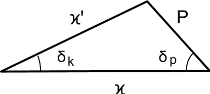
Figure 1: Triangle with the sides $\varkappa$, $\varkappa^{\prime}$, and $|{\bf P}|$.

After integration over ${{\bf k}}$ and $|{\bf k}^{\prime}|$, the master integral can be presented in the form

$${\cal I}_{mm^{\prime}}(\varkappa,\varkappa^{\prime},{\bf P})=\frac{{\displaystyle A}}{{\displaystyle 2\pi}}\sqrt{\frac{{\displaystyle\varkappa^{\prime}}}{{\displaystyle\varkappa}}}\int_{0}^{2\pi}\mathrm{e}^{\mathrm{i}[(m-m^{\prime})\varphi^{\prime}-m\psi]}\delta\left(\varkappa^{\prime}\sqrt{1+\epsilon^{2}+2\epsilon\cos\varphi^{\prime}}-\varkappa\right)\mathrm{d}\varphi^{\prime},$$ (12)

where

$$A=\mathrm{i}^{m^{\prime}-m}\;e^{i(m-m^{\prime})\varphi_{P}}\,,\;\;\psi=\arctan{\frac{{\displaystyle\epsilon\sin{\varphi^{\prime}}}}{{\displaystyle 1+\epsilon\cos{\varphi^{\prime}}}}}\,,\;\;\epsilon=\frac{{\displaystyle|{\bf P}|}}{{\displaystyle\varkappa^{\prime}}}$$ (13)

and $\varphi_{P}$ is the azimuthal angle of the momentum transfer ${\bf P}$. The differential cross section is proportional to $|{\cal I}_{mm^{\prime}}(\varkappa,\varkappa^{\prime},{\bf P})|^{2}$. It is this quantity whose $m^{\prime}$ distribution and $\varkappa^{\prime}$-dependence determines the OAM properties of the final twisted state.

In the case of strictly forward scattering, ${\bf P}=0$, one immediately obtains

$${\cal I}_{mm^{\prime}}(\varkappa,\varkappa^{\prime},0)=\delta(\varkappa-\varkappa^{\prime})\delta_{mm^{\prime}}\,.$$ (14)

This result means that in the strictly forward scattering the twisted quantum numbers $m$ and $\varkappa$ are transferred from the initial to the final particle without any change, [5].

The master integral for the non-zero transverse momentum transfer, which was calculated in [12], is equal to

$${\cal I}_{mm^{\prime}}(\varkappa,\varkappa^{\prime},{\bf P})=\frac{{\displaystyle A}}{{\displaystyle 2\pi}}\frac{{\displaystyle\sqrt{\varkappa\varkappa^{\prime}}}}{{\displaystyle\Delta}}\,\cos[m^{\prime}\delta_{k}-(m-m^{\prime})\delta_{p}]\,,$$ (15)

where $\Delta={1\over 2}\varkappa\varkappa^{\prime}\sin\delta_{k}$ is just the area of the triangle with sides $\varkappa$, $\varkappa^{\prime}$, $|{\bf P}|$ shown in Fig. 1, and

$$\delta_{k}=\arccos\left({\varkappa^{2}+\varkappa^{\prime 2}-{\bf P}^{2}\over 2\varkappa\varkappa^{\prime}}\right)\,,\quad\delta_{p}=\arccos\left({\varkappa^{2}+{\bf P}^{2}-\varkappa^{\prime 2}\over 2\varkappa|{\bf P}|}\right)$$ (16)

are its angles. One sees that the $m^{\prime}$-dependence of the differential cross section comes from the oscillating cosine squared:

$$|{\cal I}_{mm^{\prime}}(\varkappa,\varkappa^{\prime},{\bf P})|^{2}\propto\cos^{2}[m^{\prime}\delta_{k}-(m-m^{\prime})\delta_{p}]\,.$$ (17)

At very large $m^{\prime}$ this cosine is a strongly oscillating function of the moduli of the momenta and it can be replaced by $1/2$. Therefore, the contribution of arbitrarily large $m^{\prime}$ is not suppressed.

As already said above, in an accurate analysis one must keep the cylindric quantization volume of radius $R$ large but finite. In this case, the differential cross section receives approximately homogeneous contribution from the entire $m^{\prime}$-region

$$-m_{max}\mathrel{\hbox to0.0pt{\lower 4.0pt\hbox{\hskip 1.0pt$\sim$}\hss}\raise 1.0pt\hbox{$<$}}m^{\prime}\mathrel{\hbox to0.0pt{\lower 4.0pt\hbox{\hskip 1.0pt$\sim$}\hss}\raise 1.0pt\hbox{$<$}}m_{max}\,,\quad m_{max}=\varkappa^{\prime}R\,.$$ (18)

Contribution of each partial wave with a given $m^{\prime}$ is suppressed by $1/m_{max}$, so it is the summation

$${1\over m_{max}}\sum_{m^{\prime}=-m_{max}}^{m_{max}}|{\cal I}_{mm^{\prime}}(\varkappa,\varkappa^{\prime},{\bf P})|^{2}$$

that stays constant in the $R\to\infty$ limit. Therefore, in this limit we recover the result (2) found in [12].

On the other hand, one can investigate the small momentum transfer approximation inside the master integral. Denoting $|{\bf P}|=\epsilon\varkappa^{\prime}$ and assuming $\epsilon\ll 1$, one can represent expression (12) as

$${\cal I}_{mm^{\prime}}(\varkappa,\varkappa^{\prime},{\bf P})\approx\frac{{\displaystyle A}}{{\displaystyle 2\pi}}\int_{0}^{2\pi}e^{\mathrm{i}[(m-m^{\prime})\varphi^{\prime}-m\epsilon\sin\varphi^{\prime}]}\,\delta(\varkappa^{\prime}-\varkappa+\varkappa^{\prime}\epsilon\cos\varphi^{\prime})\,d\varphi^{\prime}\,.$$ (19)

Note that although $\epsilon\ll 1$, the value of $m\epsilon$ in the exponential can be large. We then perform the formal small-$\epsilon$ expansion of the delta-functional under the integral

$$\delta(\varkappa^{\prime}-\varkappa^{\prime}+\varkappa^{\prime}\epsilon\cos\varphi^{\prime})=\delta(\varkappa^{\prime}-\varkappa)+\varkappa^{\prime}\epsilon\cos\varphi^{\prime}\cdot\delta^{\prime}(\varkappa^{\prime}-\varkappa)+{\it o}(\epsilon)\,,$$ (20)

which is valid on a class of sufficiently smooth functions of $\varkappa$ or $\varkappa^{\prime}$, and keep only the first term. This leads us to the approximate value for the master integral

$${\cal I}_{mm^{\prime}}(\varkappa,\varkappa^{\prime},{\bf P})=A\,\delta(\varkappa^{\prime}-\varkappa)J_{m-m^{\prime}}(m\epsilon)\,,$$ (21)

which clearly shows a smooth transition to the strictly forward/backward case (14). From the properties of the Bessel functions, namely that $J_{n}(x)$ is strongly suppressed at $x<n$, one can infer that at small but non-zero transverse momentum transfer ${\bf P}$ the quantum numbers $m^{\prime}$ stay close to $m$, and the result (1) follows, [5].

2.3 The origin of the discrepancy

A careful inspection shows that discrepancy between the results (1) and (2) is linked to the transverse spatial extent of the incoming twisted state.

First of all, as it was already discussed in [12], the discontinuous non-forward to forward transition is a consequence of the infinite transverse size of the pure Bessel-beam state. If the radius $R$ of the quantization volume is kept large but finite, then the smooth transition is restored in an extremely narrow region of $|{\bf P}|\sim 1/R$. This suggests that if one replaces the pure twisted initial state $|\varkappa,m\rangle$ with a wave packet

$$|i\rangle=\int_{0}^{\infty}d\varkappa\,f(\varkappa)|\varkappa,m\rangle\,,$$ (22)

with a narrow weight function $f(\varkappa)$ peaked at $\varkappa=\varkappa_{0}$ and having a width $\sigma\ll\varkappa_{0}$, then the non-forward to forward transition is expected to be smooth even for infinite $R$ and to take place within the transverse momentum transfer region $|{\bf P}|\sim\sigma$.

On the other hand, the derivation of (1) just reproduced involves manipulation of the delta-functional, which is valid only if a convolution with a sufficiently smooth function of $\varkappa$ or $\varkappa^{\prime}$ is assumed. The pure Bessel states lack such a convolution, therefore this result cannot be expected to hold for the pure Bessel states. However, for a sufficiently compact wave packet this conclusion can be valid.

These observations necessitate a careful re-analysis of the master integral for a situation when the initial state is described by a wave packet (22) rather than a pure Bessel state.

3 Scattering of a twisted wave packet

3.1 Qualitative features

Let us start by discussing qualitative features of the coordinate space wave function of the wave packet (22). When quantitative estimates are needed, we will use the gaussian approximation for the weight function $f(\varkappa)$:

$$f(\varkappa)=N\exp\left[-\frac{{\displaystyle(\varkappa-\varkappa_{0})^{2}}}{{\displaystyle 2\sigma^{2}}}\right]\,,$$ (23)

with $\sigma\ll\kappa_{0}$ and the normalization coefficient $N$ fixed by

$$\int_{0}^{\infty}|f(\varkappa)|^{2}\,\mathrm{d}\varkappa=1\,.$$ (24)

The transverse coordinate wave function $\psi_{m}(r)$ of this wave packet is defined by

$$\int_{0}^{\infty}d\varkappa f(\varkappa)\,\psi_{\varkappa m}({\bf r})={e^{im\varphi_{r}}\over\sqrt{2\pi}}\int_{0}^{\infty}\sqrt{\varkappa}d\varkappa J_{m}(\varkappa r)f(\varkappa)\equiv{e^{im\varphi_{r}}\over\sqrt{2\pi}}\psi_{m}(r)$$ (25)

and is normalized to unity:

$$\int_{0}^{\infty}rdr\,|\psi_{m}(r)|^{2}=1\,.$$ (26)

In Appendix we study some properties of this averaged wave function. We show there that if $m$ is not too large, $m\ll\varkappa_{0}^{2}/\sigma^{2}$, the wave function $\psi_{m}(r)$ exhibits radial oscillations characteristic of the Bessel function $J_{m}(\varkappa_{0}r)$ until $r$ becomes larger than the coherence radius $r_{c}=1/\sigma$. Beyond this radius, the averaged wave function is strongly suppressed. This behavior is well seen in Fig. 2 where we plotted $\psi_{5}(r)$ for $\sigma=\varkappa_{0}/5$ and $\sigma=\varkappa_{0}/20$ for $\varkappa_{0}=1$ (in arbitrary units) and compared it with the pure Bessel state $\sqrt{\varkappa_{0}}J_{5}(\varkappa_{0}r)$. However, if $m\gg\varkappa_{0}^{2}/\sigma^{2}$, there is no room left for the radial oscillations, and the wave function is strongly peaked at $r=m/\varkappa_{0}$.

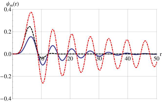
Figure 2: Radial wave functions for $m=5$ and $\varkappa_{0}=1$: the pure Bessel state $\sqrt{\varkappa_{0}}J_{5}(\varkappa_{0}r)$ (dash-dotted line), the function $\psi_{m}(r)$ for $\sigma=1/20$ (solid line), the function $\psi_{m}(r)$ for $\sigma=1/5$ (dashed line).

The effective regularization of the radial wave function by the coherence radius $r_{c}=1/\sigma$ plays an important role in the master integral and its $m^{\prime}$-dependence. The master integral (2.2) for the pure twisted states can be also represented as a triple-Bessel integral, see [12]:

$${\cal I}_{mm^{\prime}}(\varkappa,\varkappa^{\prime},{\bf P})=A\sqrt{\varkappa\varkappa^{\prime}}\int_{0}^{\infty}rdr\,J_{m}(\varkappa r)J_{m^{\prime}}(\varkappa^{\prime}r)J_{m-m^{\prime}}(|{\bf P}|r)\,.$$ (27)

If $m^{\prime}$ is extremely large, the main contribution comes from the large $r$-region, $r\mathrel{\hbox to0.0pt{\lower 4.0pt\hbox{\hskip 1.0pt$\sim$}\hss}\raise 1.0pt\hbox{$>$}}\mathrm{max}(m^{\prime}/\varkappa^{\prime},m^{\prime}/|{\bf P}|)$. A pure Bessel function for the initial state, $J_{m}(\varkappa r)$, is not sufficiently suppressed at such large $r$. However, if the initial state is a wave packet, then the exponential suppression is at work beyond $r_{c}$, which effectively limits the values of $|m-m^{\prime}|$.

3.2 Averaged master integral

Since the master integral is a linear functional of the initial wave function, the averaged master integral can be represented as

$${\cal I}_{mm^{\prime}}(\varkappa^{\prime},{\bf P})=\int_{0}^{\infty}d\varkappa\,{\cal I}_{mm^{\prime}}(\varkappa,\varkappa^{\prime},{\bf P})f(\varkappa)$$ (28)

or, using Eq. (12), as

$${\cal I}_{mm^{\prime}}(\varkappa^{\prime},{\bf P})=\frac{{\displaystyle A}}{{\displaystyle 2\pi}}\int_{0}^{2\pi}\mathrm{e}^{\mathrm{i}[(m-m^{\prime})\varphi^{\prime}-m\psi]}\frac{{\displaystyle f\left(\varkappa^{\prime}\sqrt{1+\epsilon^{2}+2\epsilon\cos\varphi^{\prime}}\right)}}{{\displaystyle\left(1+\epsilon^{2}+2\epsilon\cos\varphi^{\prime}\right)^{1/4}}}\mathrm{d}\varphi^{\prime}\,.$$ (29)

In this Section we aim at resolving the discrepancy between the results (1) and (2). Therefore, it is sufficient to consider non-zero but very small momentum transfer, $|{\bf P}|=\epsilon\varkappa^{\prime}$ with $\epsilon\ll 1$. In this case $\varkappa$ changes in the small interval from $\varkappa^{\prime}-|{\bf P}|$ to $\varkappa^{\prime}+|{\bf P}|$ and the averaged master integral can be approximated as

$${\cal I}_{mm^{\prime}}(\varkappa^{\prime},{\bf P})\approx\frac{{\displaystyle A}}{{\displaystyle 2\pi}}\int_{0}^{2\pi}\mathrm{e}^{\mathrm{i}[(m-m^{\prime})\varphi^{\prime}-\epsilon m\sin\varphi^{\prime}]}\,f\left(\varkappa^{\prime}+|{\bf P}|\cos\varphi^{\prime}\right)\mathrm{d}\varphi^{\prime}\,.$$ (30)

Figure 3: The weight function as a function of $x$ in the narrow peak (left) and broad peak (right) regimes.

For the further analysis we need to distinguish two cases depending on the shape of $f(\varkappa^{\prime}+|{\bf P}|\cos\varphi^{\prime})$ as a function of $x\equiv\cos\varphi^{\prime}$ on the interval $[-1,1]$:

$$f(\varkappa^{\prime}+x|{\bf P}|)=N\exp\left[-{(x-x_{0})^{2}\over 2\Delta_{x}^{2}}\right]\,,\quad x_{0}\equiv{\varkappa_{0}-\varkappa^{\prime}\over|{\bf P}|}\,,\quad\Delta_{x}\equiv{\sigma\over|{\bf P}|}\,.$$ (31)

If it is strongly peaked as in Fig. 3, left, we are dealing with the narrow-peak situation. It corresponds to $|x_{0}|<1$ and $\Delta_{x}\ll 1$:

$$\mbox{narrow peak:}\quad\sigma\ll|{\bf P}|\ll\varkappa_{0}\,.$$ (32)

In this case the relevant integrals can be taken approximately using Laplace method. The opposite case, $\Delta_{x}\gg 1$, corresponds to the broad-peak situation shown in Fig. 3, right:

$$\mbox{broad peak:}\quad|{\bf P}|\ll\sigma\ll\varkappa_{0}\,.$$ (33)

In this case the integrals can be approximately calculated by using the Taylor expansion of the weight function.

Let us derive the $m^{\prime}$ distribution in the broad and narrow peak situations. In the broad peak case, as the first approximation, one can put $f\left(\varkappa^{\prime}+|{\bf P}|\cos{\varphi^{\prime}}\right)\approx f\left(\varkappa^{\prime}\right)$ and immediately obtain the result

$${\cal I}_{mm^{\prime}}(\varkappa^{\prime},{\bf P})\approx A\,f\left(\varkappa^{\prime}\right)\,\;J_{m-m^{\prime}}(\epsilon m)\,.$$ (34)

Using the properties of the Bessel functions, one can deduce that $m^{\prime}$ should always stay close to $m$, otherwise the contribution is suppressed. For small values of $m$, when $m\epsilon\ll 1$, the only significant contribution comes from $m^{\prime}=m$. For large $m$, when $m\epsilon\gg 1$, the $m^{\prime}$-distribution is spread over several values around $m^{\prime}\approx m$.

For the narrow peak case, $|m-m^{\prime}|\gg m\epsilon$ still holds almost in the entire $m^{\prime}$ region. Then, we can read off (30) that the averaged master integral effectively extracts the $(m-m^{\prime})$-th Fourier harmonic of the weight function. Since the weight function has a peak with a width $\Delta_{x}$, we conclude that

$$|m-m^{\prime}|\mathrel{\hbox to0.0pt{\lower 4.0pt\hbox{\hskip 1.0pt$\sim$}\hss}\raise 1.0pt\hbox{$<$}}{1\over\Delta_{x}}={|{\bf P}|\over\sigma}\,.$$ (35)

This means that the final $m^{\prime}$ can strongly differ from and be much larger than the initial $m$ if $\sigma$ is sufficiently small. Considering additionally the region $|m-m^{\prime}|\mathrel{\hbox to0.0pt{\lower 4.0pt\hbox{\hskip 1.0pt$\sim$}\hss}\raise 1.0pt\hbox{$<$}}m\epsilon$ does not change this conclusion.

3.3 Different limits

The key quantity which we discuss in this Section is the $m^{\prime}$-distribution of the scattering matrix element at small ${\bf P}$. Our analysis reveals that the answer to this question depends in fact on a subtle interplay between two different limits: $\sigma\to 0$ and $|{\bf P}|\to 0$. The apparently conflicting results (1) and (2) simply correspond to two different choices of which limit is taken first.

If the initial wave packet is fixed (i.e. $\sigma$ is kept constant) and $|{\bf P}|\to 0$, then we are in the broad-peak regime, and the result (1) follows. In this way we study the non-forward to forward transition for a wave packet of fixed size. This implicit assumption, although not mentioned in [5], is essential when deriving this result.

On the contrary, if $|{\bf P}|$ is kept constant but $\sigma$ decreases, we enter the narrow-peak regime, and (35) holds. In the $\sigma\to 0$ limit we recover the result (2). This limit corresponds to the point-by-point analysis of the small-$|{\bf P}|$ behaviour in the scattering of true Bessel states, studied in [12]. This resolves the discrepancy mentioned in the introduction.

4 Orbital helicity of the final twisted state

In the previous Section we reconciled results (1) and (2) which was a technical rather than physical problem. However our calculations did not answer the physically important question: what are the true OAM properties of the final twisted state with respect to its own propagation direction?

The results of the previous Section imply that if the momentum transfer $|{\bf P}|\gg\varkappa$, a very broad $m^{\prime}$-region contributes to the differential cross section. However, this broad region can easily be an artefact of using the same $z$ axis to describe both the initial and the final twisted states. Indeed, (7) shows that a non-forward plane wave, when expanded in the basis of twisted states with respect to axis $z$, involves all values of $m$ from minus to plus infinity, despite the fact that it actually carries no OAM at all. As it was suggested in [12], for the full resolution of this problem one needs to introduce the concept of orbital helicity: the projection of orbital angular momentum not on the reaction axis $z$ but on the axis of the average propagation direction of the final particle. This is what we do in the present Section.

4.1 Orbital helicity distribution: pure Bessel states

Let us consider again the scattering process

$$|\varkappa,m\rangle_{\vec{n}}+|PW(\vec{p})\rangle\to|\varkappa^{\prime},m^{\prime}\rangle_{\vec{n}^{\prime}}+|PW(\vec{p}^{\prime})\rangle$$ (36)

with fixed $\varkappa$, $(\vec{k}\vec{n})\equiv k_{z}$, $m$ and fixed 3-momentum transfer $\vec{P}\equiv\vec{p}^{\prime}-\vec{p}$. The twisted states in (36) are defined with respect to two different axes. The incoming state is written with respect to the direction $\vec{n}$ which coincides with the axis $z$. The final twisted state is defined with respect to another direction $\vec{n}^{\prime}\not=\vec{n}$ to be defined below. The average value of the 3-momentum in the initial and final states are

$$\langle\vec{k}\rangle\equiv\langle\varkappa,m|\vec{k}|\varkappa,m\rangle=k_{z}\vec{n}\,,\quad\langle\vec{k}^{\prime}\rangle\equiv\langle\varkappa^{\prime},m^{\prime}|\vec{k}^{\prime}|\varkappa^{\prime},m^{\prime}\rangle=k^{\prime}_{z^{\prime}}\vec{n}^{\prime}\,.$$ (37)

Note that $k^{\prime}_{z^{\prime}}$ means here the component of the vector $\vec{k}^{\prime}$ along the axis $z^{\prime}$ directed along $\vec{n}^{\prime}$.

A priori, any choice of the axis $\vec{n}^{\prime}$ is allowed. We find it convenient to use the following prescription: we draw $\vec{n}^{\prime}$ along the direction of the well-defined 3-momentum $\vec{q}\equiv\langle\vec{k}\rangle-\vec{P}\equiv q\vec{n}^{\prime}$. Note that although $\vec{q}$ and $\langle\vec{k}^{\prime}\rangle$ are parallel, they are not equal, $q\not=k^{\prime}_{z^{\prime}}$, because the averaged momenta are not supposed to obey any conservation law

$$\langle\vec{k}\rangle\not=\langle\vec{k}^{\prime}\rangle+\vec{P}\,.$$ (38)

In this way the quantity $m^{\prime}$ becomes the orbital helicity rather than just OAM projection on an arbitrary axis.

We now aim at evaluating the master integral for this scattering. When calculating the scattering matrix element for the process (36), we have a very familiar expression for the master integral:

$${\tilde{\cal I}}_{mm^{\prime}} \equiv 2\pi\,\delta(k_{z}-k^{\prime}_{z}-P_{z})\cdot{\cal I}_{mm^{\prime}}(\kappa,\kappa^{\prime},{\bf P})$$ (39)

$$= i^{m^{\prime}-m}\sqrt{\varkappa\varkappa^{\prime}}\int_{0}^{2\pi}d\varphi d\varphi^{\prime}\,e^{i(m\varphi-m^{\prime}\varphi^{\prime})}\,\cdot\delta^{(3)}(\vec{k}-\vec{k}^{\prime}-\vec{P})\,.$$

Notice two important differences with respect to the “coaxial” master integral (2.2). First, the azimuthal angles $\varphi$ and $\varphi^{\prime}$ lie in two different planes which are orthogonal to $\vec{n}$ and $\vec{n}^{\prime}$, respectively. Second, the master integral contains 3-dimensional delta-function instead of just two-dimensional: since the integration is not limited to a single transverse plane, the longitudinal delta-function is, naturally, included in the integral.

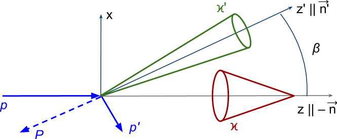
Figure 4: Kinematics and choice of the axes for the off-forward twisted particle scattering.

The integral (39) can be easily done in the usual cartesian coordinate frame $(x,y,z)$. This frame is fixed in the following way (see Fig. 4). The directions $\vec{n}$ and $\vec{n}^{\prime}$ define the axis $z$ and the $(x,z)$ plane. The axis $y$ is orthogonal to the plane containing $\vec{n}$, $\vec{n}^{\prime}$, $\vec{P}$. In this coordinate frame the momenta $\vec{k}$ and $\vec{P}$ are

$$\vec{k}=\left(\begin{array}[]{c}\varkappa\cos\varphi\\ \varkappa\sin\varphi\\ k_{z}\end{array}\right)\,,\quad\vec{P}=\left(\begin{array}[]{c}P_{x}\\ 0\\ P_{z}\end{array}\right)\,,$$ (40)

with $P_{x}<0$. The direction of $\vec{n}^{\prime}$ is $(\sin\beta,0,\cos\beta)$, which is defined by

$$\vec{q}\equiv\langle\vec{k}\rangle-\vec{P}=\left(\begin{array}[]{c}-P_{x}\\ 0\\ k_{z}-P_{z}\end{array}\right)=q\left(\begin{array}[]{c}\sin\beta\\ 0\\ \cos\beta\end{array}\right)\,,$$ (41)

where $q^{2}=P_{x}^{2}+(k_{z}-P_{z})^{2}$. Then, the momentum $\vec{k}^{\prime}$ has components

$$\vec{k}^{\prime}=\left(\begin{array}[]{c}\varkappa^{\prime}c_{\beta}c_{\varphi^{\prime}}+k^{\prime}_{z^{\prime}}s_{\beta}\\ \varkappa^{\prime}s_{\varphi^{\prime}}\\ -\varkappa^{\prime}s_{\beta}c_{\varphi^{\prime}}+k^{\prime}_{z^{\prime}}c_{\beta}\end{array}\right)\,,$$ (42)

where we introduced the obvious short-hand notation for sines and cosines.

The three-dimensional delta-function in (39) expresses the conservation of the three-momentum at the level of plane waves: $\vec{k}=\vec{k}^{\prime}+\vec{P}$. Writing it explicitly, we obtain

$$\delta^{(3)}(\vec{k}-\vec{k}^{\prime}-\vec{P}) = \delta(\varkappa c_{\varphi}-\varkappa^{\prime}c_{\beta}c_{\varphi^{\prime}}-(k^{\prime}_{z^{\prime}}-q)s_{\beta})$$ (43)

$$\times \delta(\varkappa s_{\varphi}-\varkappa^{\prime}s_{\varphi^{\prime}})\cdot\delta(\varkappa^{\prime}s_{\beta}c_{\varphi^{\prime}}-(k^{\prime}_{z^{\prime}}-q)c_{\beta})\,.$$

In order for the integral to be non-zero, we require that

$$\varkappa^{\prime}s_{\beta}\geq|k^{\prime}_{z^{\prime}}-q|c_{\beta}\,.$$ (44)

Then the $z$-delta-function can be used to kill the $\varphi^{\prime}$ integration. Let us for the moment drop the $\exp(im\varphi-im^{\prime}\varphi^{\prime})$ factor from the master integral (39). Then we have

$$\int d\varphi d\varphi^{\prime}\delta^{(3)}(\vec{k}-\vec{k}^{\prime}-\vec{P})$$ (45)

$$= {2\over s_{\beta}}\int d\varphi\,\delta(\varkappa^{\prime 2}s^{2}_{\varphi^{\prime}}-\varkappa^{2}s^{2}_{\varphi})\ \delta\!\left(\varkappa c_{\varphi}-{k^{\prime}_{z^{\prime}}-q\over s_{\beta}}\right)$$

$$= {2\over s_{\beta}}\ \delta\!\left[\varkappa^{\prime 2}+(k^{\prime}_{z^{\prime}}-q)^{2}-\varkappa^{2}\right]\int d\varphi\ \delta\!\left(\varkappa c_{\varphi}-{k^{\prime}_{z^{\prime}}-q\over s_{\beta}}\right)$$

$$= {2\over\sqrt{\varkappa^{\prime 2}-\varkappa^{2}\cos^{2}\beta}}\ \delta\!\left[\varkappa^{\prime 2}+(k^{\prime}_{z^{\prime}}-q)^{2}-\varkappa^{2}\right]\,.$$

Here we implicitly assumed that the integration over $\varphi$ goes not around the full $2\pi$ domain, but only over the semicircle where $\sin\varphi$ has the same sign as $\sin\varphi^{\prime}$. The extra delta-function in (45) replaces $\delta(k_{z}-k^{\prime}_{z}-P_{z})$ in the “coaxial” case. Here it leads to important conclusions that

$$\varkappa^{\prime}\leq\varkappa\,,\quad|k^{\prime}_{z^{\prime}}-q|\leq\varkappa\,.$$ (46)

So, the values of the momentum transfer ${\vec{P}}$ (both $P_{x}$ and $P_{z}$) can be large, $|P_{x,z}|\gg\varkappa$, but they must be accompanied by a correspondingly large value of $k^{\prime}_{z^{\prime}}$.

It is convenient to introduce the “angle” $\xi$ by

$$\varkappa^{\prime}\equiv\varkappa\cos\xi\,,\quad k^{\prime}_{z^{\prime}}-q=\varkappa\sin\xi\,,\quad\xi\in[-\pi/2,\pi/2]\,.$$ (47)

In this notation condition (44) becomes

$$\sin(\beta-|\xi|)\geq 0\quad\to\quad\beta\geq|\xi|\,.$$ (48)

which also implies $\varkappa^{2}\geq\varkappa^{\prime 2}\geq\varkappa^{2}\cos^{2}\beta$. The pair of values of $\varphi$ and $\varphi^{\prime}$, which are set by the delta-functions, can be written as

$$\cos\varphi={\sin\xi\over\sin\beta}\,,\quad\cos\varphi^{\prime}={\tan\xi\over\tan\beta}\,.$$ (49)

Let us now recall that the master integral (39) contains the exponential factor $\exp(im\varphi-im^{\prime}\varphi^{\prime})$. Since the integral just taken receives its contribution only from two $(\varphi,\varphi^{\prime})$ points, this extra factor is simply an overall multiplier computed at each of these two points. Effectively, it corresponds to the replacement $2\to 2\cos(m\varphi-m^{\prime}\varphi^{\prime})$. Thus, the final result for the master integral is

$${\tilde{\cal I}}_{mm^{\prime}}=i^{m^{\prime}-m}\sqrt{\varkappa\varkappa^{\prime}}\cdot 2{\cos(m\varphi-m^{\prime}\varphi^{\prime})\over\sqrt{\varkappa^{\prime 2}-\varkappa^{2}\cos^{2}\beta}}\ \delta\!\left[\varkappa^{\prime 2}+(k^{\prime}_{z^{\prime}}-q)^{2}-\varkappa^{2}\right]\,,$$ (50)

where the values of $\varphi$ and $\varphi^{\prime}$ are given by (49). This expression shows the final orbital helicity $m^{\prime}$ distribution. Similarly to the “coaxial” case, ${\tilde{\cal I}}_{mm^{\prime}}$ is an oscillatory function of $m^{\prime}$. Clearly, $|\tilde{\cal I}_{mm^{\prime}}(\varkappa,\varkappa^{\prime})|^{2}$ is not suppressed even at extremely large $m^{\prime}$. However, this is an artefact of taking pure Bessel beams for the initial and final twisted states. In reality, a pure Bessel state is as unphysical as a plane wave, because its radial coordinate wave function effectively extends to infinity and is not normalizable. Even if $m$ is small, all values of $m^{\prime}$ up to infinity contribute to the cross section.

4.2 Orbital helicity distribution: wave packets

The above conclusion is expected to change if the initial and final twisted states are assumed to be a wave packets rather than pure Bessel states. As before, we represent the initial and final twisted states similarly to (25): initial twisted state as a superposition of $|\varkappa,m\rangle$ states with equal value of $m$ and different values of $\varkappa$ (distributed by the weight function $f(\varkappa)$ around $\varkappa_{0}$ in a region with width $\sigma$) and final twisted state as a superposition of $|\varkappa^{\prime},m^{\prime}\rangle$ states with equal value of $m^{\prime}$ and different values of $\varkappa^{\prime}$ (distributed by the weight function $g(\varkappa^{\prime})$ around $\varkappa^{\prime}_{0}$ in a region with width $\sigma^{\prime}$).

Then we calculate the averaged master integral

$${\tilde{\cal I}}_{mm^{\prime}}^{av}=\int d\varkappa f(\varkappa)\int d\varkappa^{\prime}g(\varkappa^{\prime})\,{\tilde{\cal I}}_{mm^{\prime}}(\varkappa,\varkappa^{\prime})\,.$$ (51)

Since the initial laser photon is assumed to be monocromatic, the final photon has a fixed energy, $\omega^{\prime}=E+\omega-E^{\prime}$, therefore, the longitudinal momenta

$$k_{z}=\sqrt{\omega^{2}-\varkappa^{2}}\,,\;\;k^{\prime}_{z^{\prime}}=\sqrt{(\omega^{\prime})^{2}-(\varkappa^{\prime})^{2}}$$ (52)

change when $\varkappa$ and $\varkappa^{\prime}$ are varied.

Let us first use the $\varkappa^{\prime}$ integration to eliminate the delta-function. Manipulation with delta-function gives:

$$\delta\!\left[\varkappa^{\prime 2}+(k^{\prime}_{z^{\prime}}-q)^{2}-\varkappa^{2}\right]=\delta\left(\varkappa^{2}-\omega^{\prime 2}-q^{2}+2q\sqrt{\omega^{\prime 2}-\varkappa^{\prime 2}}\right)=\frac{{\displaystyle q^{2}+\omega^{\prime 2}-\varkappa^{2}}}{{\displaystyle 8qD}}\,\delta\left(\varkappa^{\prime}-\frac{{\displaystyle 2D}}{{\displaystyle q}}\right)\,,$$

where

$$D=\frac{{\displaystyle 1}}{{\displaystyle 4}}\sqrt{2\left(\varkappa^{2}\omega^{\prime 2}+\omega^{\prime 2}q^{3}+q^{2}\varkappa^{2}\right)-\varkappa^{4}-\omega^{\prime 4}-q^{4}}\,.$$

After the $\varkappa^{\prime}$ integration we obtain

$${\tilde{\cal I}}_{mm^{\prime}}^{av}=\int d\varkappa f(\varkappa)g(\varkappa^{\prime})\,i^{m^{\prime}-m}\sqrt{\frac{{\displaystyle\varkappa}}{{\displaystyle\varkappa^{\prime}}}}\cdot 2{\cos(m\varphi-m^{\prime}\varphi^{\prime})\over\sqrt{\varkappa^{\prime 2}-\varkappa^{2}\cos^{2}\beta}}\;\frac{{\displaystyle q^{2}+\omega^{\prime 2}-\varkappa^{2}}}{{\displaystyle 4q^{2}}}$$ (53)

with $\varkappa^{\prime}=2D/q$.

The resulting expression for ${\tilde{\cal I}}^{av}_{mm^{\prime}}$ can be easily analyzed in the case of small-angle scattering, $\beta\ll 1$, which implies $|\xi|\leq\beta\ll 1$ and $\varphi\approx\varphi^{\prime}$. As the result, the cosine becomes simply

$${\cos[(m-m^{\prime})\arccos(\xi/\beta)]\over\sqrt{\cos^{2}\xi-\cos^{2}\beta}}={T_{m^{\prime}-m}(\xi/\beta)\over\sqrt{\beta^{2}-\xi^{2}}},$$ (54)

where $T_{n}(x)$ is the Chebyshev’s polynomial of the first kind:

$$\cos(n\cdot\arccos(x))=T_{n}(x)\,.$$

The integral is then proportional to

$$\int d\varkappa f(\varkappa)g(\varkappa^{\prime})\;\frac{{\displaystyle T_{m^{\prime}-m}(\xi/\beta)}}{{\displaystyle\sqrt{\beta^{2}-\xi^{2}}}}=\int d\xi\,F(\xi)\;\frac{{\displaystyle T_{m^{\prime}-m}(\xi/\beta)}}{{\displaystyle\sqrt{\beta^{2}-\xi^{2}}}}\,,$$ (55)

where $F(\xi)$ includes both weight functions and the Jacobian of the $\varkappa\to\xi$ change of variables.

This Chebyshev polynomial makes $(m^{\prime}-m)/4$ oscillations on the interval $\xi/\beta$ from $-1$ to $1$. Smearing of $\varkappa$ due to the weight function leads to smearing of $\xi/\beta$ by the amount of $\Delta\xi/(8\beta)$. Therefore, if $|m^{\prime}-m|\gg 8\beta/\Delta\xi$, the oscillations strongly suppress the contribution. We conclude that only $m^{\prime}$ such that

$$|m^{\prime}-m|\mathrel{\hbox to0.0pt{\lower 4.0pt\hbox{\hskip 1.0pt$\sim$}\hss}\raise 1.0pt\hbox{$<$}}\frac{{\displaystyle 8\beta}}{{\displaystyle\Delta\xi}}$$ (56)

effectively contribute to the cross section.

Let us estimate $\Delta\xi$ using expression

$$\xi\approx\frac{{\displaystyle k^{\prime}_{z^{\prime}}-q}}{{\displaystyle\varkappa}}$$ (57)

obtained from Eq. (47). From here we have

$$\Delta\xi\approx\frac{{\displaystyle\Delta k^{\prime}_{z^{\prime}}-\Delta q}}{{\displaystyle\varkappa}}-\frac{{\displaystyle k^{\prime}_{z^{\prime}}-q}}{{\displaystyle\varkappa^{2}}}\,\Delta\varkappa\approx-\frac{{\displaystyle\Delta q}}{{\displaystyle\varkappa}}\approx\frac{{\displaystyle\Delta\varkappa}}{{\displaystyle\omega}}\approx\frac{{\displaystyle\sigma}}{{\displaystyle\omega}}\,,$$ (58)

since the following estimations are valid from (52) at $\omega\ll\omega^{\prime}$ and $\varkappa^{\prime}\approx\varkappa$:

$$\Delta k_{z}\approx-\frac{{\displaystyle\varkappa\Delta\varkappa}}{{\displaystyle\omega}}\,,\;\;\Delta k^{\prime}_{z^{\prime}}\approx-\frac{{\displaystyle\varkappa^{\prime}\Delta\varkappa^{\prime}}}{{\displaystyle\omega^{\prime}}}\ll\Delta k_{z}\,,$$ (59)

and therefore,

$$\Delta q=\Delta\sqrt{(k_{z}-P_{z})^{2}+P_{x}^{2}}=\frac{{\displaystyle(k_{z}-P_{z})\Delta k_{z}}}{{\displaystyle q}}\approx-\frac{{\displaystyle\varkappa}}{{\displaystyle\omega}}\,\Delta\varkappa\,.$$ (60)

As a result, we obtain the important estimate:

$$|m^{\prime}-m|\mathrel{\hbox to0.0pt{\lower 4.0pt\hbox{\hskip 1.0pt$\sim$}\hss}\raise 1.0pt\hbox{$<$}}8\,\beta\;\frac{{\displaystyle\omega}}{{\displaystyle\sigma}}\,.$$ (61)

Note that the right hand side of this inequality can be small for small enough angles $\beta$.

A crucial observation is that the result (61) does not require the transverse momentum transfer $|{\bf P}|$ to be small (smaller than $\varkappa_{0}$ or even $\sigma$ as it was the case in the previous Section). The only assumption for this simple analysis was that the scattering angle was much smaller than one. We remind once again that for the Compton scattering, where the region of small scattering angles $\beta\sim m_{e}/E_{e}$ gives the dominant contribution to the total cross section, this approximation is fully valid.

Therefore, we proved that if the initial and final twisted states are the wave packets, then final orbital helicity $m^{\prime}$ stays close to $m$ and the final $\varkappa^{\prime}$ stays close to $\varkappa$ during small-angle scattering.

5 Conclusions

Photons carrying non-zero orbital angular momentum are now routinely produced in the low-energy domain. It was recently argued in [5, 6] that Compton backscattering of photons with OAM can help create high-energy photons carrying large values of OAM. Intermediate energy electrons with large OAM have been recently created experimentally, and the same technique can in principle be used to give twist to other particles, such as protons. Thus, energetic particles with OAM and their scattering can become a new promising tool in experimental subatomic physics.

In these circumstances, it is essential to understand quantum-field-theoretically how the OAM of a particles changes after its scattering. In particular, the vital question about the OAM of the final twisted photon scattered at non-zero angle, which arises in the context of Compton backscattering, has not been satisfactorily answered so far. Two previous analyzes, [5] and [12], led to conflicting results. In order to resolve this controversy and to answer the question, one needs to generalize the formalism and to allow the initial twisted state to be in the form of a wave packet rather than a pure Bessel state. This generalization of the formalism is done in the present paper. Using it, we completely resolve the existing controversy by showing that the two apparently conflicting results emerge in two different limits of the same expression.

Another key part of this work is the concept of orbital helicity of a twisted particle: that is, the OAM projection on its averaged propagation direction rather than on the reaction axis. With this more physically appealing definition we derived the orbital helicity distribution of a generic scalar scattering at any angle. Our results confirm the intuitive expectation that the orbital helicity is approximately conserved at small-angle scattering.

Appendix A Wave packets of Bessel states

Here, for the sake of completeness, we study the radial wave function (25) of the Bessel-beam wave packet in some detail.

Let us start with its expected qualitative behaviour if $m$ is not too large. As $r$ grows, the radial oscillations of different twisted states in the wave packed remain almost in phase up to the coherence radius $r_{c}=1/\sigma$, and at $r>r_{c}$ destructive interference strongly suppresses the wave function. However, at extremely large radii the true large-$r$ asymptotics determined by the small-$\varkappa$ behavior of the weight function sets in.

The calculations below show that this qualitative picture changes when $m\mathrel{\hbox to0.0pt{\lower 4.0pt\hbox{\hskip 1.0pt$\sim$}\hss}\raise 1.0pt\hbox{$>$}}\varkappa_{0}^{2}/\sigma^{2}$. Depending on whether $m$ is larger or smaller than $\varkappa_{0}^{2}/\sigma^{2}$, we will speak of the small-$m$ and large-$m$ regions.

To study the shape of $\psi_{m}(r)$, we break it into three $r$-regions: the central hole, $\varkappa_{0}r<m$, the intermediate region, $\varkappa_{0}r\gg m$, and the true large-$r$ asymptotics, which sets in at $r>r_{*}$ to be determined below. In the first two regions, the approximate forms of the Bessel functions allow us to represent $\psi_{m}(r)$ as

$$\psi_{m}(r)\approx N\sqrt{2\pi}\sigma\sqrt{\varkappa_{0}}J_{m}(\varkappa_{0}r)\times\left\{\begin{array}[]{lcl}\exp\left[-\frac{{\displaystyle\sigma^{2}(m+1/2)^{2}}}{{\displaystyle 2\varkappa_{0}^{2}}}\right]&\mbox{at}&\varkappa_{0}r\mathrel{\hbox to0.0pt{\lower 4.0pt\hbox{\hskip 1.0pt$\sim$}\hss}\raise 1.0pt\hbox{$<$}}m\,,\\[11.38109pt] \exp\left[-\frac{{\displaystyle\sigma^{2}r^{2}}}{{\displaystyle 2}}\right]&\mbox{at}&\varkappa_{0}r\gg m\,.\end{array}\right.$$ (62)

These shapes come from the region under the peak in the weight function $f(\varkappa)$ which is assumed to be its dominating feature.

The very far asymptotics of $\psi_{m}(r)$ comes from the small-$\varkappa$ behaviour of $f(\varkappa)$. For example, if $f(0)$ is finite, then $f(0)$ can be taken out of the integral, and we are left with an integral of the form of

$$I(y)=\int_{0}^{y}dx\sqrt{x}J_{m}(x)\,.$$ (63)

The large $y$ behavior of this intregral is

$$I(y)\approx\sqrt{2}{\Gamma\left({3\over 4}+{m\over 2}\right)\over\Gamma\left({1\over 4}+{m\over 2}\right)}-\sqrt{{2\over\pi}}\cos\left(y-{\pi\over 2}m+{\pi\over 4}\right)+{\cal O}(y^{-1})\,.$$

The first term is very close to $\sqrt{m}$ at all $m\geq 1$, while the second term is a small amplitude oscillatory function. Thus, a reasonable estimate for the large-$r$ asymptotics of the wave function is

$$\psi_{m}(r)\approx N\,\exp\left[-{\varkappa_{0}^{2}\over 2\sigma^{2}}\right]\cdot{\sqrt{m}\over r^{3/2}}\,.$$ (64)

where the exponentially suppressed factor is simply $f(0)$. Note that the exact $r$-power is driven by the $f(\varkappa)$ behaviour in the $\varkappa\to 0$ limit; the asymptotics $\psi_{m}(r)\propto r^{-3/2}$ is a consequence of the finite $f(0)$.

By comparing (62) and (64), one finds that the true large-$r$ asymptotics sets in beyond

$$r_{*}={\varkappa_{0}\over\sigma^{2}}\gg r_{c}={1\over\sigma}\,.$$ (65)

The intermediate region exists if $r_{*}\gg m/\varkappa_{0}$. Therefore, the qualitative picture described above holds if $m\gg\varkappa_{0}^{2}/\sigma^{2}$, that is, in the small-$m$ region.

For very large $m$, there is no room for the intermediate $r$-region. The radius at which the Bessel function $J_{m}$ is supposed to have its first peak is already so large, that destructive interference takes place. Therefore, the wave function exhibits no radial oscillations and has the shape of a single peak at $r=m/\varkappa_{0}$. Its shape can be estimated to be

$$\psi_{m}(r)\propto{\sqrt{\varkappa_{0}}\over r}\exp\left[-{(m-\varkappa_{0}r)^{2}\over 2r^{2}\sigma^{2}}\right]\approx{\varkappa_{0}^{3/2}\over m}\exp\left[-{(r-m/\varkappa_{0})^{2}\over 2\Delta^{2}}\right]\,,$$ (66)

with $\Delta=m\sigma/\varkappa_{0}^{2}$ (so that $\Delta/r=\sigma/\varkappa_{0}$).

References

• [1] L. Allen et al., Phys. Rev. A 45, 8185 (1992).
• [2] S. Franke-Arnold, L. Allen, M. Padgett, Laser and Photonics Reviews 2, 299 (2008).
• [3] “Twisted photons (Application of light with orbital angular momentum)”, edited by J.P. Torres and L. Torner, Wiley-VCH, (2011).
• [4] J. E. Curtis, B. A. Koss, and D. G. Gries, Opt. Commun. 207, 169 (2002)
• [5] U. D. Jentschura and V. G. Serbo, Phys. Rev. Lett. 106, 013001 (2011) [arXiv:1008.4788 [physics.acc-ph]].
• [6] U. D. Jentschura and V. G. Serbo, Eur. Phys. J.  C71, 1571 (2011). [arXiv:1101.1206 [physics.acc-ph]].
• [7] V. G. Nedorezov, A. A. Turinge, Y. M. Shatunov, Phys. Uspekhi 47, 341 (2004).
• [8] K. Yu. Bliokh et al., Phys. Rev. Lett. 99, 190404 (2007).
• [9] K. Yu. Bliokh and A. S. Desyatnikov, Phys. Rev. A 79, 011807(R) (2009).
• [10] M. Uchida and A. Tonomura, Nature 464, 737 (2010).
• [11] J. Verbeeck, H. Tian, P. Schlattschneider, Nature 467, 301 (2010); B. J. McMorran et al, Science 331, 192 (2011).
• [12] I. P. Ivanov, Phys. Rev. D 83, 093001 (2011) [arXiv:1101.5575 [hep-ph]].