Scaling study of the gluon propagator in Coulomb gauge QCD on isotropic and anisotropic lattices

Abstract

We calculate the transverse and time-time components of the instantaneous gluon propagator in Coulomb gauge QCD by using an SU(3) quenched lattice simulation on isotropic and anisotropic lattices. We find that the gluon propagators suffer from strong discretization effects on the isotropic lattice; on the other hand, those on the anisotropic lattices give a better scaling. Moreover, on these two type of lattices the transverse parts are significantly suppressed in the infrared region and have a turnover at about 500 [MeV]. The high resolution to the temporal direction due to the anisotropy yields small discretization errors for the time-time gluon propagators, which also show an infrared enhancement as expected in the Gribov-Zwanziger confinement scenario.

I Introduction

The Coulomb gauge with no negative metric provides a very clear physical picture in the sense that the color-Gauss’s law can be formally solved, only transverse degrees of freedom appear as dynamical degrees of freedom, and Fock space is well defined. The prominent feature taking the Coulomb gauge is that an instantaneous interaction, which is requisite for color confinement, shows up in the Hamiltonian. In the Gribov-Zwanziger scenario, the path integral is dominated by the configurations near the Gribov horizon where the lowest eigenvalue of the Faddeev-Popov (FP) ghost operator vanishes Zwanziger (1994). The lattice simulations show the enhancement of near-zero modes of the FP eigenvalues Greensite et al. (2005); Nakagawa et al. (2007). Accordingly, the color-Coulomb instantaneous interaction bears a confining force. It has been also confirmed by the lattice simulations that the color-Coulomb potential rises linearly at large distances and its string tension is larger than the string tension of the static Wilson potential Greensite and Olejnik (2003); Nakamura and Saito (2006); Nakagawa et al. (2006, 2008), which is expected from the Zwanziger’s inequality Zwanziger (2003). In addition, the color-Coulomb potential can be reevaluated by inverting the FP ghost matrix and this analysis has shown that its string tension almost saturates the Wilson string tension Voigt et al. (2008).

Exploring the gluon propagator is a central issue for studying the confinement mechanism in QCD. The transverse would-be physical gluon propagator is expected to be suppressed in the infrared (IR) region due to the proximity of the Gribov region in the IR direction in the Gribov-Zwanziger scenario Zwanziger (1991). There have been a lot of lattice studies and functional analyses in the Landau gauge (see, for instance, LABEL:Bogolubsky:2009dc,Fischer:2008uz and references therein). Contrastingly, there are few lattice studies on the instantaneous gluon propagator in the Coulomb gauge Cucchieri and Zwanziger (2001a); Langfeld and Moyaerts (2004); Burgio et al. (2009); Nakagawa et al. (2009). In the continuum theory, on the other hand, there are many works on the variational approach in the Coulomb gauge, which are very useful to study the spectrum of the hadronic bound states and the Green’s functions Szczepaniak and Swanson (2001); Szczepaniak (2004); Feuchter and Reinhardt (2004); Epple et al. (2007, 2008); Campagnari and Reinhardt (2008), in addition to the functional analysis Watson and Reinhardt (2008); Reinhardt and Watson (2009); Watson and Reinhardt (2009).

The Coulomb gauge fixing condition is imposed on each time slice and it does not introduce correlations between neighboring time slices. Accordingly, the equal-time correlation between gauge fields at different points

$$\langle A^{a}_{\mu}(\vec{x},t)A^{b}_{\nu}(\vec{y},t)\rangle$$ (1)

is well defined in the Coulomb gauge. Recent lattice studies of the instantaneous gluon propagator revealed that it shows scaling violation Burgio et al. (2009); Nakagawa et al. (2009); namely, the gluon propagator calculated at different lattice couplings do not fall on top of one curve after multiplicative renormalization.

In order to circumvent the problem of scaling violation, the authors of LABEL:Burgio:2008jr have extracted the instantaneous gluon propagator by eliminating the $p_{4}$ dependence of the unequal-time propagator. It has been concluded that the instantaneous transverse gluon propagator $D^{\rm tr}(\vec{p})$ is multiplicatively renormalizable in the Hamiltonian limit and the numerical data of it are well fitted with the Gribov-type form of the propagator

$$D^{\rm tr}(\vec{p})=\frac{1}{2\sqrt{\lvert\vec{p}\rvert^{2}+\frac{M^{2}}{\lvert\vec{p}\rvert^{2}}}},$$ (2)

where $M$ is a fitting parameter at which the propagator shows a turnover. The method was applied to the transverse gluon propagator successfully both in 2+1 and 3+1 dimensional SU(2) Yang-Mills theory Burgio et al. (2010, 2009) while it does not improve the scaling violation of the temporal gluon propagator since the time-time component of the unequal-time gluon propagator is energy independent even after the residual gauge fixing Quandt et al. (2008).

As another approach, a new momentum cut is introduced in LABEL:Nakagawa:2009zf in addition to the cone cut and the cylinder cut. High momentum data that suffer from discretization errors are excluded from the analysis of the instantaneous propagators by this new cut. Combined with the matching analysis given in LABEL:Leinweber:1998uu, it has been shown that this procedure successfully reduces the scaling violation for the transverse gluon propagator, but it fails for the time-time component of the gluon propagator.

In this study, we take a different route to show that the instantaneous gluon propagator is multiplicatively renormalizable. The problem of scaling violation of the instantaneous propagator can be seen even at the tree level with a finite temporal lattice spacing as was discussed in LABEL:Burgio:2008jr (we shall briefly review the point in Appendix B). The reason is that the energy integral does not run from $-\infty$ to $\infty$ but from $-\pi/a_{\tau}$ to $\pi/a_{\tau}$ on a finite lattice, and this introduces the spurious $\lvert\vec{p}\rvert$ dependence on the free instantaneous propagator. Therefore, we expect that the instantaneous propagator is multiplicatively renormalizable in the Hamiltonian limit $a_{\tau}\to 0$. To make this point clear, we calculate the transverse and the time-time components of the instantaneous gluon propagator on anisotropic lattices and show how the scaling violation becomes milder as the anisotropy increases, i.e., as we get close to the Hamiltonian limit.

The organization of this paper is as follows. In the subsequent sections, we describe the lattice observables, the space and time components of the instantaneous gluon propagator, and the lattice setup of our numerical simulations. In Secs. IV and V, the numerical results of the transverse and the temporal components of the instantaneous propagators on the isotropic lattice are reported. Section VI is devoted to show the results for the transverse propagator on the anisotropic lattices. In the subsequent Secs. VII, we discuss the IR and the ultraviolet (UV) behavior of the propagator by making the power law fitting. The anisotropic lattice results for the temporal gluon propagator are given in Sec. VIII, and the IR and the UV fittings are examined in Sec. IX. We attempt to extract the color-Coulomb string tension from the instantaneous temporal gluon propagator in position space in Sec. X. The conclusions are drawn in Sec. XI.

II Instantaneous gluon propagator

We calculate the transverse and the time-time components of the instantaneous gluon propagator,

$$D^{ab}_{\mu\nu}(\vec{x}-\vec{y})=\langle A^{a}_{\mu}(\vec{x},t)A^{b}_{\nu}(\vec{y},t)\rangle,$$ (3)

in the momentum space,

$$D^{ab}_{ij}(\vec{p})=\delta^{ab}\left(\delta_{ij}-\frac{p_{i}p_{j}}{\lvert\vec{p}\rvert^{2}}\right)D^{\rm tr}(\vec{p}),$$ (4)

$$D^{ab}_{44}(\vec{p})=\delta^{ab}\frac{Z_{44}(\vec{p})}{\lvert\vec{p}\rvert^{2}},$$ (5)

where the gauge fields are related to the link variables through

$$A^{\rm lat}_{\mu}(\vec{x},t)=\left.\frac{U_{\mu}(\vec{x},t)-U_{\mu}^{\dagger}(\vec{x},t)}{2ig_{0}a_{\mu}}\right|_{\rm traceless}.$$ (6)

The instantaneous gluon propagator is evaluated on each time slice and we average over all time slices. The lattice momenta $k_{\mu}$ are discretized and take integer values in the range $(-L_{\mu}/2,L_{\mu}/2]$. The lattice momenta and the continuum ones are related via

$$p_{\mu}=\frac{2}{a_{\mu}}\sin\left(\frac{\pi k_{\mu}}{L_{\mu}}\right),$$ (7)

where $a_{\mu}(L_{\mu})$ are $a_{\sigma}(L_{\sigma})$ for $\mu=1$ to $3$ and $a_{\tau}(L_{\tau})$ for $\mu=4$, respectively.

We note that the unequal-time propagator $D_{\mu\nu}$ has mass dimension 2 in momentum space, while the instantaneous one has mass dimension 1. This is because the instantaneous propagator is obtained by integrating the unequal-time propagator over the time component of the four momentum;

$$D_{\mu\nu}(\vec{p})=\int\frac{dp_{4}}{2\pi}D_{\mu\nu}(\vec{p},p_{4}).$$ (8)

The unrenormalized transverse gluon propagator $D^{\rm tr}_{\rm lat}$, which is measured by lattice simulations, is related to the renormalized propagator $D^{\rm tr}_{\rm R}$ via the multiplicative renormalization,

$$D^{\rm tr}_{\rm R}(\vec{p};\mu)=a_{\sigma}Z^{\rm tr}(a_{\sigma},\mu)D^{\rm tr}_{\rm lat}(\vec{p}a_{\sigma}),$$ (9)

where $\mu$ is the renormalization point. We expect that the renormalized propagator is independent of the lattice spacing in the scaling regime. As we shall see later, the multiplicative renormalizability does not hold for finite temporal lattice spacing and we have to take the Hamiltonian limit, $a_{\tau}\to 0$.

The color-Coulomb potential plays a crucial role in the Coulomb gauge QCD. It was shown that the time-time component of the gluon propagator can be decomposed into the instantaneous part and the noninstantaneous part Cucchieri and Zwanziger (2001b),

$$D_{44}(\vec{x},t)=V_{c}(\vec{x})\delta(t)+P(\vec{x},t).$$ (10)

The first term in the right-hand side represents the color-Coulomb potential, which is defined as the vacuum expectation value of the kernel of the instantaneous interaction,

$$V_{c}(\vec{x}-\vec{y})\delta^{ab}=\langle(M^{-1}[A](-\partial_{i}^{2})M^{-1}[A])^{ab}_{\vec{x},\vec{y}}\rangle.$$ (11)

Here $M^{-1}$ is the Green’s function of the Faddeev-Popov ghost operator. In Eq. (10), $P(\vec{x},t)$ is assumed to be nonsingular at $t=0$ as opposed to the first term. It has been shown that both $V_{c}$ and $P$ are renormalization-group invariant Zwanziger (1998); namely, the renormalization constant for the color-Coulomb potential can be set to be 1 in the continuum limit. We expect that the color-Coulomb potential $V_{c}$ can be extracted from the instantaneous temporal gluon propagator as

$$V_{c}(\vec{x})=a_{\tau}D_{44}(\vec{x}),$$ (12)

when we are in the scaling region and the lattice spacing is small enough, where $a_{\tau}$ comes from the $\delta$ function.

III Lattice setup

The lattice configurations are generated by the heat-bath Monte Carlo technique with the standard Wilson plaquette action,

$$S=\frac{\beta}{\xi_{B}}\sum_{n,i<j\leq 3}\operatorname{\mathfrak{Re}}\operatorname{Tr}(1-U_{ij}(n))\\ +\beta\xi_{B}\sum_{n,i\leq 3}\operatorname{\mathfrak{Re}}\operatorname{Tr}(1-U_{i4}(n)).$$ (13)

Here $U_{\mu\nu}(n)$ indicates the plaquette operator, and $\beta=2N_{c}/g_{0}^{2}$ is the lattice coupling. On the isotropic lattice, the bare anisotropy $\xi_{B}$ is 1 and the action can be written in a familiar form

$$S=\beta\sum_{n,\mu<\nu}\operatorname{\mathfrak{Re}}\operatorname{Tr}(1-U_{\mu\nu}(n)).\\$$ (14)

The renormalized anisotropy $\xi$ is defined as the ratio of the spatial lattice spacing to the temporal lattice spacing, $\xi=a_{\sigma}/a_{\tau}$. The ratio of $\xi_{B}$ and $\xi$ can be determined nonperturbatively by matching the spatial and the temporal Wilson loops on anisotropic lattices. We use the relation obtained by Klassen for the range $1\leq\xi_{B}\leq 6$ and $5.5\leq\beta\leq\infty$ Klassen (1998). We adopt the values of the lattice spacing given in LABEL:Namekawa:2001ih for $\xi=2$ and in LABEL:Matsufuru:2001cp for $\xi=4$, where the static quark potential was measured to set the scale. For the isotropic lattice, the scale is set by using the scaling relation obtained by Necco and Sommer, with the Sommer scale parameter $r_{0}=0.5$ [fm], which is applicable in the range $5.7\leq\beta\leq 6.92$ Necco and Sommer (2002).

In our simulations, the first 5000 sweeps are discarded for thermalization, and we measured the instantaneous gluon propagator for $50-100$ configurations, each of which is separated by 100 sweeps. All the lattice parameters are given in Table 1.

Table 1: The lattice couplings, the spatial and the temporal lattice extents, the lattice spacings, the lattice volumes in physical units, and the number of configurations used to evaluate the instantaneous propagators.

$\xi=a_{\sigma}/a_{\tau}$	$L_{\sigma}$	$L_{\tau}$	$\beta$	$\xi_{B}$	$a_{\sigma}^{-1}$ [GeV]	$a_{\sigma}$ [fm]	$V$[fm4]	Number of configurations
1	24	24	5.70	1	1.160	0.1702	4.094	100
	48	48	:	:	:	:	8.174	100
	56	56	:	:	:	:	9.534	100
	64	64	:	:	:	:	10.94	100
	24	24	5.80	:	1.446	0.1364	3.274	100
	24	24	6.00	:	2.118	0.0932	2.244	100
	32	32	:	:	:	:	2.984	100
	48	48	:	:	:	:	4.474	100
	56	56	:	:	:	:	5.224	100
	64	64	:	:	:	:	5.974	100
2	24	48	5.80	1.674	1.104	0.1787	4.294	80
	24	48	6.00	1.705	1.609	0.1227	2.944	80
	24	48	6.10	1.718	1.889	0.1045	2.514	80
4	16	64	5.75	3.072	1.100	0.1794	2.874	100
	24	96	:	:	:	:	4.314	50
	32	128	:	:	:	:	5.744	50
	48	192	:	:	:	:	8.614	100
	24	96	5.95	3.159	1.623	0.1216	2.924	50
	48	192	:	:	:	:	5.844	100
	24	96	6.10	3.211	2.030	0.0972	2.334	50
	32	128	:	:	:	:	3.114	50
	48	192	:	:	:	:	4.674	100

In the Coulomb gauge the transversality condition

$$\partial_{i}A_{i}(\vec{x},t)=0$$ (15)

is imposed on the gauge fields at each time slice, where $i$ runs from 1 to 3. On a lattice, gauge configurations satisfying the Coulomb gauge condition can be obtained by minimizing the functional

$$F_{U}[g]=\frac{1}{L_{\sigma}^{3}}\sum_{\vec{x},i}\operatorname{\mathfrak{Re}}\operatorname{Tr}\left(1-\frac{1}{3}g^{\dagger}(\vec{x},t)U_{i}(\vec{x},t)g(\vec{x}+\vec{i},t)\right)$$ (16)

with respect to the gauge transformation $g(\vec{x},t)\in$ SU(3) on each time slice. The functional derivative of Eq. (16) with respect to $g$ yields the transversality condition $\nabla_{i}A^{\rm lat}_{i}(\vec{x},t)=0$, where $\nabla$ is the lattice backward difference, and it reproduces the Coulomb gauge condition in the continuum limit. The Coulomb gauge fixing has been done using an iterative method with the Fourier acceleration Davies et al. (1988), and we stop the iterative gauge fixing if the violation of the transversality becomes less than $10^{-14}$;

$$\theta=\frac{1}{(N_{c}^{2}-1)L_{\sigma}^{3}}\sum_{\vec{x},a,i}(\nabla_{i}A_{i}^{\rm lat}(\vec{x},t))^{2}<10^{-14}.$$ (17)

This stopping criterion is applied for each time slice. We note that the accuracy of the gauge fixing is crucial for the transverse propagator to see the IR suppression, which is discussed in Appendix A.

In order to reduce lattice artifacts, we apply the cone and cylinder cuts to the momenta Leinweber et al. (1999). The cone cut is necessary to address finite volume effects that are seen in small momentum data. On the other hand, the cylinder cut reduces artifacts due to the broken rotational symmetry on lattice. The statistical errors are estimated by the jackknife method.

IV Instantaneous transverse gluon propagator on the isotropic lattice

Although the problem of the scaling violation for the instantaneous gluon propagator has already been discussed in Refs. Burgio et al. (2009); Nakagawa et al. (2009), we here show the lattice result for the instantaneous transverse gluon propagator on the isotropic lattice to clarify the issues. The instantaneous transverse gluon propagator on the isotropic lattice at $\beta$=5.7 and 6.0 is drawn in Fig. 1. The propagator is normalized such that $D^{\rm tr}(\lvert\vec{p}\rvert=2{\rm[GeV]})=1$.

We observe that $D^{\rm tr}$ has a maximum at $p=0.4-0.5$ [GeV] irrespective of the lattice coupling and it decreases with the momentum in the IR region. This is a striking feature of the transverse gluon propagator. The instantaneous propagator is defined as the energy integral of the unequal-time propagator,

$$D(\lvert\vec{p}\rvert)=\int\frac{dp_{4}}{2\pi}D(\vec{p},p_{4}).$$ (18)

For a massless particle and a massive particle, $D(\lvert\vec{p}\rvert)=1/(2\lvert\vec{p}\rvert)$ and $D(\lvert\vec{p}\rvert)=1/(2\sqrt{\lvert\vec{p}\rvert^{2}+m^{2}})$, respectively. Thus the instantaneous transverse propagator can be interpreted as the inverse of the energy dispersion relation of the would-be physical gluons. It implies that the propagator at vanishing momentum corresponds to the inverse of the effective mass of the gluon. The IR suppression of the instantaneous transverse gluon propagator means that the gluons have momentum dependent effective mass $M(\vec{p})$ and it diverges in the IR limit, $\lim_{\vec{p}\to 0}M(\vec{p})=\infty$, indicating the confinement of gluons.

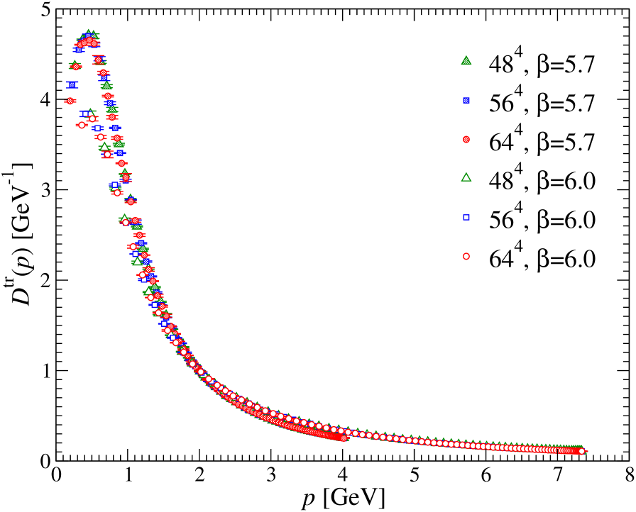
Figure 1: The instantaneous transverse gluon propagator in physical units at $\beta=5.7$ and $\beta=6.0$. The propagator is renormalized at $\lvert\vec{p}\rvert$=2 [GeV].

In addition to the bump structure of the transverse propagator, the two curves corresponding to different lattice couplings cross at the renormalization point and deviate from each other in the small and the large momentum regions. This is not seen in the Landau gauge gluon propagator (see e.g. LABEL:Leinweber:1998uu). Such a behavior of the propagator casts doubt the validity of the multiplicative renormalizability for the instantaneous gluon propagator.

Taking a closer look at the raw results of the numerical simulations gives us a clue to cure scaling violation. Assuming multiplicative renormalization for the propagator, the renormalized dressing function $Z^{\rm tr}_{\rm R}$ of the transverse gluon propagator, $Z^{\rm tr}_{\rm R}=\lvert\vec{p}\rvert D^{\rm tr}_{\rm R}$, is related to the bare unrenormalized dressing function $Z^{\rm tr}_{\rm lat}$ via

$$Z^{\rm tr}_{\rm R}(\vec{p};\mu)=Z(a_{\sigma},\mu)Z^{\rm tr}_{\rm lat}(\lvert\vec{p}\rvert a_{\sigma})$$ (19)

in the scaling regime. Here $Z(a_{\sigma},\mu)$ is a renormalization constant. It is easily read off from this relation that in the log-log plot of the dressing function of the propagator, converting from lattice units to physical units corresponds to the parallel displacement in the horizontal direction and the renormalization of $Z^{\rm tr}$ corresponds to that in the vertical direction. If the propagator is multiplicatively renormalizable, the different curves associated with the different lattice couplings can fall on top of each other by a parallel shift of the curves in the horizontal and the vertical directions in a double-log plot.

The left panel of Fig. 2 shows the dressing function of the unrenormalized transverse gluon propagator in lattice units. It is apparent that the two curves cannot coincide by adopting any scaling relation or by imposing any renormalization condition since such manipulations correspond to the horizontal and the vertical shifts in the log-log plot of the dressing function but not the rotation or deformation of the curves. Therefore, the scaling violation of the transverse gluon propagator is purely due to discretization errors.

Furthermore, we observe that the IR behavior of the dressing function at different couplings shows the same behavior, while in the UV region the slope of the curves differs. The right panel of Fig. 2, in which the dressing function renormalized at $\lvert p\rvert$=1 [GeV] is plotted as a function of the physical momentum, illuminates such a tendency; the two curves almost fall on top of each other in the IR region while the deviation between them is pronounced in the UV region. This indicates that the scaling problem of $D^{\rm tr}$ resides in the lattice data in the UV region.

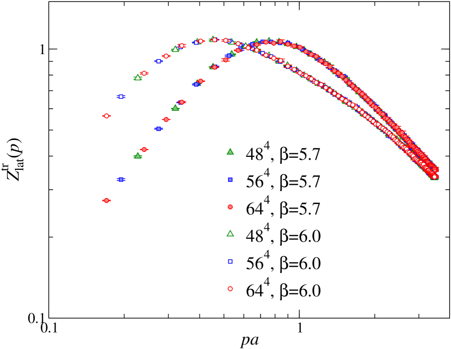
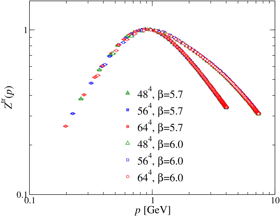
Figure 2: The dressing function of the unrenormalized instantaneous transverse gluon propagator, $Z^{\rm tr}_{\rm lat}(\vec{p})=\lvert\vec{p}\rvert D^{\rm tr}_{\rm lat}(\vec{p})$, at different lattice couplings in lattice units (left). The dressing function renormalized at $\lvert\vec{p}\rvert$=1 [GeV] in physical units (right).

This kind of behavior can be found for the instantaneous free propagator; namely, the instantaneous propagator shows the scaling violation even at the tree level (see Appendix B). It is the crucial point of the scaling violation that the instantaneous propagator is defined as the energy integral of the unequal-time propagator. For a finite temporal lattice spacing, the energy integral is limited in the interval $[-\pi/a_{\tau},\pi/a_{\tau}]$, and it induces a spurious $\lvert\vec{p}\rvert$ dependence on the instantaneous propagator. It leads the discretization errors especially at large momenta, as demonstrated in Appendix B, while it disappears only in the Hamiltonian limit $a_{\tau}\to 0$. Accordingly, the lattice data in the UV region for the instantaneous transverse gluon propagator suffer from the discretization errors that cannot be eliminated with the cylinder cut or the cone cut we applied.

One way to circumvent this problem is to exclude the high momentum data from the analysis of the propagator. This has been studied in LABEL:Nakagawa:2009zf combined with the matching procedure proposed in LABEL:Leinweber:1998uu in order to find a reasonable value for the available momentum range. It has been shown that the instantaneous transverse gluon propagator shows scaling behavior by restricting the available momentum range. The data on large lattices shown in Fig. 2 illustrate that the discretization errors are relatively small in the IR region, and this supports the validity of the prescription in LABEL:Nakagawa:2009zf. The another way is to calculate the unequal-time propagator $D(\vec{p},p_{4})$ and eliminates the $p_{4}$ dependence of $D(\vec{p},p_{4})$ as was discussed in LABEL:Burgio:2008jr, and the instantaneous transverse gluon propagator has been shown to be multiplicatively renormalizable.

V Instantaneous temporal gluon propagator on the isotropic lattice

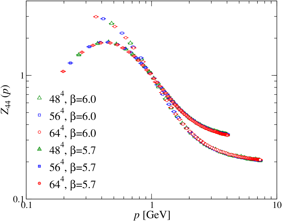
Figure 3: The dressing function of the instantaneous temporal gluon propagator in physical units at $\beta=5.7$ and $\beta=6.0$. The renormalization point is set to be 2 [GeV] in the left panel and 1[GeV] in the right panel.

In this section, we discuss the isotropic lattice result for the temporal gluon propagator. The dressing function of the instantaneous temporal gluon propagator on the isotropic lattice at $\beta$=5.7 and 6.0 is drawn in Fig. 3. The dressing function is normalized such that $Z_{44}(\lvert\vec{p}\rvert=2{\rm[GeV]})=1$ in the left panel and $Z_{44}(\lvert\vec{p}\rvert=1{\rm[GeV]})=1$ in the right panel. The dressing function $Z_{44}$ is constant for $\lvert\vec{p}\rvert$ at the tree level. In the Gribov-Zwanziger scenario, this is expected to diverge in the IR limit resulting in the confining behavior of the color-Coulomb potential, which is necessary condition for color confinement in Coulomb gauge QCD.

Although the scaling violation is clearly visible in $Z_{44}$ as in the transverse gluon propagator, the scaling issue is worse for the temporal gluon propagator than the transverse one. In the case of $D^{\rm tr}$, the IR data do not much suffer from the discretization errors and they almost fall on top of each other by setting the renormalization point to a small momentum. Contrastingly, the discrepancy between two data sets of $Z_{44}$ corresponding to different lattice spacings remains both in the IR and the UV regions by changing the renormalization point (compare the left and the right panels of Fig. 3). Indeed, the scaling violation of $D_{44}$ is not settled by the $\alpha$-cut method employed in LABEL:Nakagawa:2009zf, indicating that the data at small momenta may also be affected by the discretization errors.

Besides the scaling violation, we observe that the dressing function is suppressed in the IR region. For the temporal gluon propagator, we expect that its instantaneous part behaves as $1/\lvert\vec{p}\rvert^{4}$ in the IR region since it corresponds to the color-Coulomb potential, which rises linearly with distance between a quark and an antiquark Greensite and Olejnik (2003); Nakamura and Saito (2006). As opposed to our expectation, the numerical results on the isotropic lattice show that the dressing function $Z_{44}$ decreases with momentum in the IR region for the coarser lattice.

The unexpected IR suppression of $Z_{44}$ may stem from an incomplete isolation of the instantaneous part in $D_{44}$. The unequal-time temporal gluon propagator can be decomposed into the instantaneous part and the vacuum polarization part as Eq. (10) in the continuum theory, and it gives

$$\int^{\epsilon}_{-\epsilon}dtD_{44}(\vec{x},t)=V(\vec{x})+O(\epsilon).$$ (20)

On a lattice with finite $a_{\tau}$, $\epsilon$ is of the order of $a_{\tau}$ and we would have a $O(a_{\tau})$ contribution from the polarization term in the instantaneous $D_{44}$ on the lattice. The unwanted suppression at small momenta may originate from such a contribution of the polarization term, and furthermore, the energy integral of the polarization term would produce a spurious $\lvert\vec{p}\rvert$ dependence as for the transverse gluon propagator, which leads the scaling violation.

Before closing the section, we summarize the points so far: (1) The transverse gluon propagator on the isotropic lattice suffers from the discretization errors at large momenta and it can be ascribed to the spurious $\lvert\vec{p}\rvert$ dependence coming from the temporal lattice cutoff in the energy integral defining the instantaneous propagator. (2) The temporal gluon propagator is affected both in the IR and the UV regions by the discretization errors, and it may stem from the $O(a_{\tau})$ contribution of the polarization term in the instantaneous propagator besides the limited energy integral.

VI Instantaneous transverse gluon propagator on anisotropic lattices

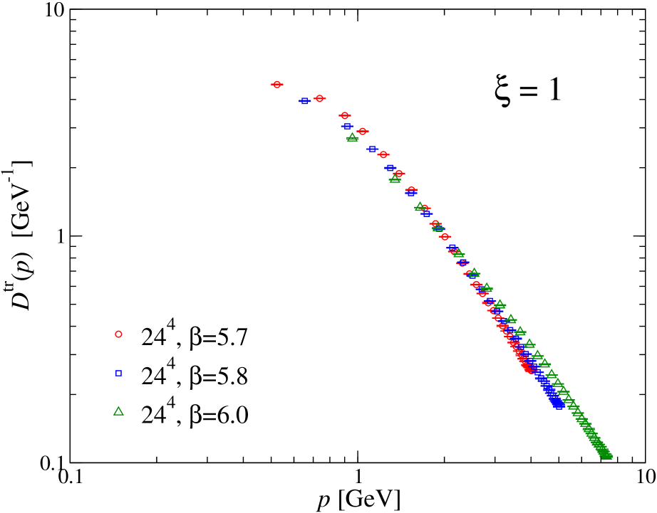
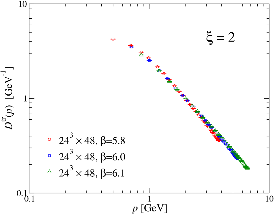
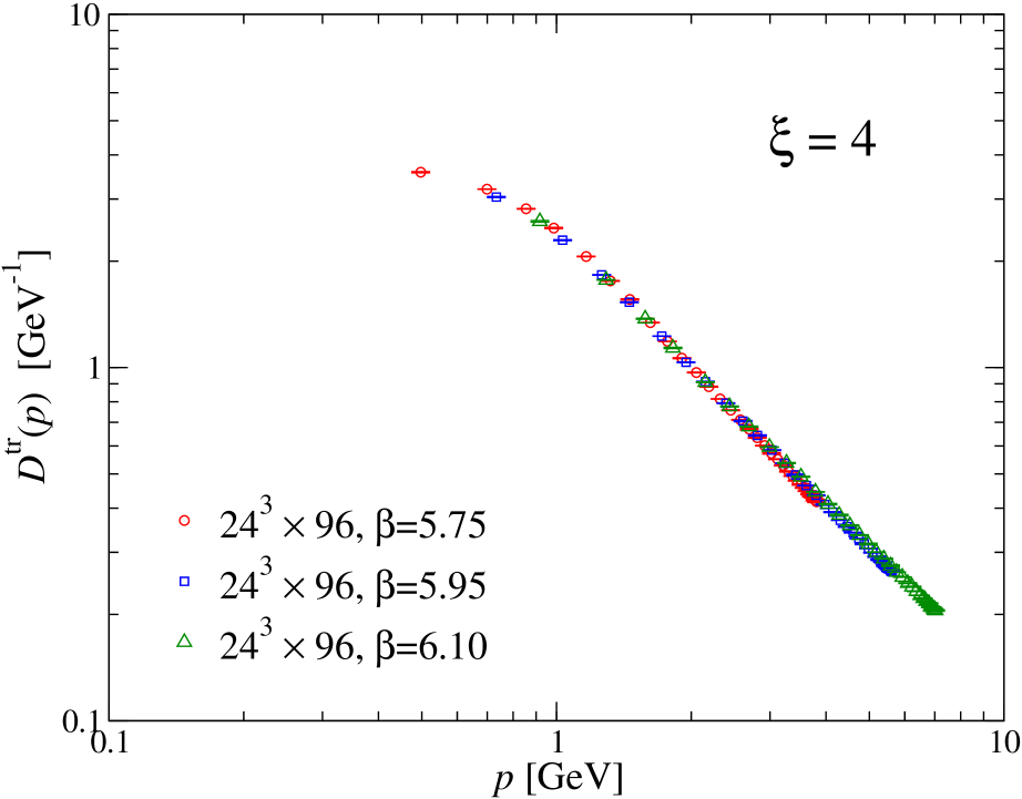
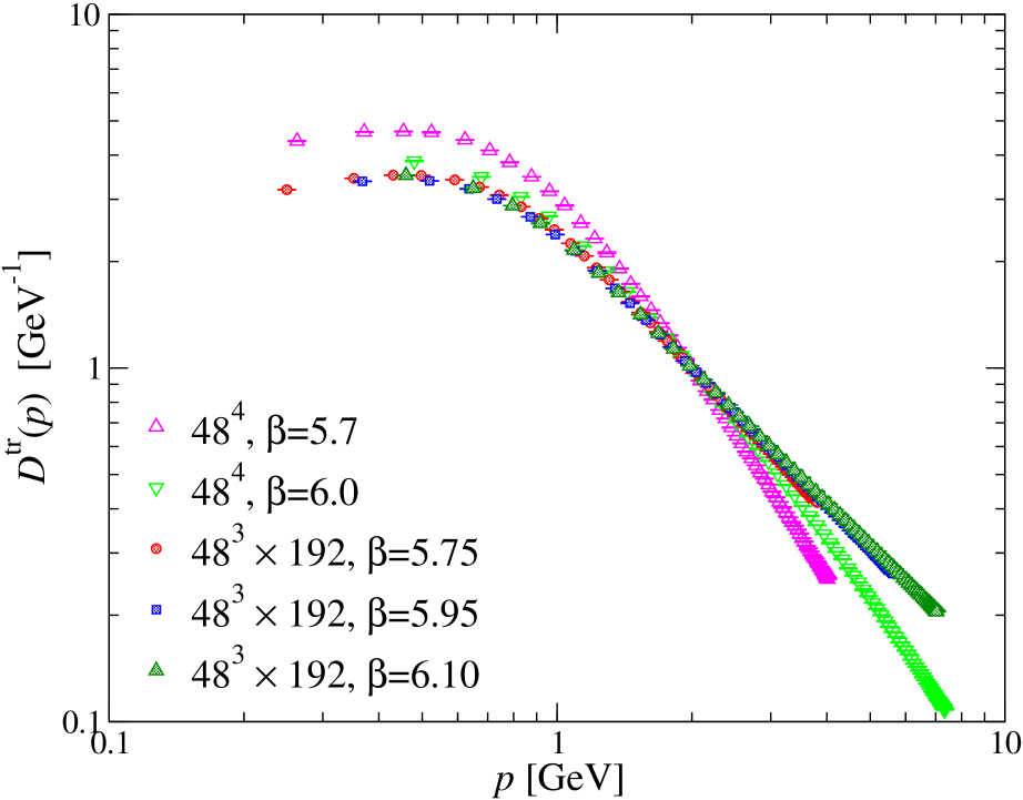
Figure 4: The instantaneous transverse gluon propagator on the isotropic lattice (top left), on the anisotropic lattices with $\xi=2$ (bottom left), and with $\xi=4$ (top right). The results for the isotropic lattice and the anisotropic lattice with $\xi=4$ on the large lattice volume are drawn together in one figure for direct comparison (bottom right). The propagator is renormalized to unity at $\lvert\vec{p}\rvert=2$ [GeV].

The instantaneous transverse gluon propagators for several anisotropies are drawn in Fig. 4. Compared to the isotropic case, the deviations of three curves corresponding to different lattice couplings become moderate on the anisotropic lattice with $\xi=2$. Further increase of $\xi$ leads to a nice scaling behavior and the data points for $\xi=4$ almost fall on top of one curve. Accordingly, our results on the anisotropic lattices support our expectation that scaling violation observed in the instantaneous transverse gluon propagator disappears in the limit $\xi\to\infty$ ($a_{\tau}\to 0$).

In order to investigate how scaling violation is cured by getting close to the Hamiltonian limit, we quantify the difference of two curves by the following function,

$$\chi^{2}=\sum_{i=1}^{n_{\rm f}}\left(\frac{D_{\rm f}(p_{i})-D_{\rm c}^{\rm int}(p_{i})}{\sigma_{{\rm f},i}}\right)^{2}+\sum_{i=1}^{n_{\rm c}}\left(\frac{D_{\rm c}(p_{i})-D_{\rm f}^{\rm int}(p_{i})}{\sigma_{{\rm c},i}}\right)^{2}.$$ (21)

$D_{\rm f}(p_{i})$ represents the measured value of the propagator at the momentum $p_{i}$ and $\sigma_{{\rm f},i}$ the corresponding statistical error. $D_{\rm c}^{\rm int}(p_{i})$ is the estimated value obtained by a cubic spline interpolation of the other lattice data set $D_{\rm c}$. The subscripts f and c label two different data sets, meaning “finer” and “coarser”. The summations extend over the data points at which the two lattice data sets overlap in the momentum.

We compute $\chi^{2}$ defined above for the following data sets:

(1)	$(24^{3}\times 48,\beta=5.80,\xi=2)$	and	$(24^{3}\times 48,\beta=6.00,\xi=2)$
(2)	$(24^{3}\times 96,\beta=5.75,\xi=4)$	and	$(24^{3}\times 96,\beta=5.95,\xi=4)$.

We note that the physical volumes are very similar; (1) $V\sim 4.29^{4}$ [fm⁴] and $V\sim 2.94^{4}$ [fm⁴], and (2) $V\sim 4.31^{4}$ [fm⁴] and $V\sim 2.92^{4}$ [fm⁴], respectively. For each case, we found

(1)	$\chi^{2}/N_{\rm DF}=867$
(2)	$\chi^{2}/N_{\rm DF}=309$,

where $N_{\rm DF}$ is the number of degrees of freedom of the $\chi^{2}$ analysis. Decreasing the temporal lattice spacing by a factor of 2, $\chi^{2}/N_{\rm DF}$ reduces by about a factor 3. We note that the absolute value of $\chi^{2}$ is unimportant since it depends on the absolute value of the propagator, which can take an arbitrarily large (or small) value by multiplicative renormalization. $\chi^{2}$ defined above make sense only when we compare the $\chi^{2}$ values under the same renormalization condition and the fixed ratio of the physical volumes of the lattice data sets to be analyzed.

In the right bottom panel of Fig. 4, the instantaneous transverse gluon propagator on the spatial lattice extent $L_{\sigma}=48$ is plotted both for the isotropic lattice and the $\xi=4$ anisotropic lattice. We observe that the propagator has a maximum at about 500 [MeV] irrespective of the lattice coupling and the anisotropy, and it decreases with the momentum in the IR region. Accordingly, the turnover of the transverse gluon propagator survives in the Hamiltonian limit.

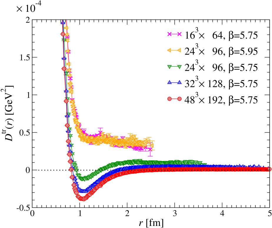
Figure 5: The unrenormalized instantaneous gluon propagator in position space (the correlation function of the gauge fields) on $\xi=4$ anisotropic lattice. The physical volumes are $2.87^{4}$ [fm⁴] (crosses), $2.92^{4}$ [fm⁴] (left triangles), $4.31^{4}$ [fm⁴] (down triangles), $5.74^{4}$ [fm⁴] (up triangles), and $8.61^{4}$ [fm⁴] (circles).

The confined behavior of the gluon propagator can be seen more directly in position space. The unrenormalized correlation function of the transverse gauge fields on the anisotropic lattice $\xi=4$ is depicted in Fig. 5. On small lattices (crosses and left triangles in the figure), the correlation function is positive and a decreasing function of the distance. As the physical volume increases, $D^{\rm tr}(r)$ develops a dip at about $r=1$ [fm] and becomes negative around the dip. On the largest volume, the correlation function quickly decreases with distance at small $r$ and becomes negative in the range $r\sim 1-2$ [fm] and then vanishes at large distances. It means that the gauge fields have no correlation over the hadronic scale in sharp contrast to the massless particles for which the correlation function behaves as $1/r^{2}$. We notice that the results at the approximately fixed physical volume nicely agree with each other; namely, lattice discretization errors do not seriously affect the correlation function on the anisotropic lattice.

VII Power law fitting of $D^{\rm tr}$ at small and large momenta

We note that the momentum dependence of the instantaneous transverse gluon propagator on the anisotropic lattices in the UV region significantly differs from that on the isotropic lattice (see the bottom right panel in Fig. 4). On the isotropic lattice, the slope at high momenta gets smaller as the lattice couplings increase. On the anisotropic lattices, the slope decreases further. In order to investigate the UV behavior of the transverse gluon propagator, we make the power law ansatz,

$$D^{\rm tr}(\vec{p})=\frac{d_{1}}{\lvert\vec{p}\rvert^{1+\gamma_{\rm gl}^{\rm UV}}},$$ (22)

and fit this ansatz to the data on $24^{3}\times L_{\tau}$ lattices in the momentum range $\lvert\vec{p}\rvert\geq 6$ [GeV]. The fitted parameters are given in Table 2. We see that $\gamma_{\rm gl}^{\rm UV}$ gets small values as the anisotropy increases, and that for $\xi=4$ takes about one third of that on the isotropic lattice.

As we have discussed in Sec. IV, the inverse of the instantaneous propagator can be interpreted as the energy dispersion relation. Since gluons are expected to behave as free massless particles at sufficiently large momentum due to asymptotic freedom, this interpretation can be allowed if the instantaneous transverse gluon propagator behaves as $1/\lvert\vec{p}\rvert$ in the UV region, which corresponds to the null UV exponent. Therefore, the decrease of $\gamma_{\rm gl}^{\rm UV}$ with increasing $\xi$ is consistent with the asymptotic free field behavior of the gluon fields in the continuum limit .

Table 2: The result of the UV power law fitting of $D^{\rm tr}$ in the momentum range $\lvert\vec{p}\rvert\geq 6$ [GeV].

$(L_{\sigma},L_{\tau},\xi,\beta)$	$d_{1}$	$\gamma_{\rm gl}^{\rm UV}$	$\chi^{2}/N_{\rm DF}$
(24, 24, 1, 6.0)	4.89(14)	0.920(15)	1.34
(24, 48, 2, 6.1)	3.83(25)	0.617(35)	0.86
(24, 96, 4, 6.1)	2.49(7)	0.282(15)	0.68

In order to explore the IR behavior of the instantaneous transverse gluon propagator, we make the power law ansatz,

$$D^{\rm tr}(\vec{p})=d_{2}\lvert\vec{p}\rvert^{\gamma_{\rm gl}^{\rm IR}},$$ (23)

in the IR region. The fitted parameters are listed in Table 3.

Although the fitting becomes worse and the IR exponent $\gamma^{\rm IR}_{\rm gl}$ becomes small as the maximum momentum of the fitting range increases, $\gamma^{\rm IR}_{\rm gl}$ takes a positive value in all the cases. For the anisotropic lattice, we need much larger lattices to extract the IR exponent with an acceptable $\chi^{2}$ value. In both the isotropic and the anisotropic cases, our result of the IR fitting predicts the vanishing transverse gluon propagator at zero momentum. Given the fact that the fitted values of $\gamma^{\rm IR}_{\rm gl}$ increases with decreasing the maximum momentum of the fitting range, the $\gamma^{\rm IR}_{\rm gl}$ values listed in Table 3 would give a lower bound for the IR exponent of the transverse gluon propagator in the Coulomb gauge.

We note that fitting the transverse gluon propagator with the Gribov-type ansatz, Eq. (2), which successfully reproduced the lattice data in LABEL:Burgio:2008jr, did not work in our lattice data for both the isotropic and the anisotropic cases. At the same time, the peak position of the transverse gluon propagator differs between our results and the results in LABEL:Burgio:2008jr; it is about 500 [MeV] in our case and the fitting analysis in LABEL:Burgio:2008jr gives 880(10) [MeV], which is rather close to the peak position of the dressing function $Z^{\rm tr}$ in our results (see the right panel of Fig. 2). It deserves further study to clarify whether this discrepancy comes from the gauge group [SU(3) in this study and SU(2) in LABEL:Burgio:2008jr] or the adopted prescriptions to circumvent scaling violation.

Table 3: The result of the IR power law fitting of $D^{\rm tr}$. $\lvert\vec{p}_{max}\rvert$ represents the maximum momentum of the fitting range.

$(L_{\sigma},\xi,\beta)$	$\lvert\vec{p}_{max}\rvert$	$d_{2}$	$\gamma_{\rm gl}^{\rm IR}$	$\chi^{2}/N_{\rm DF}$
	0.27	6.64(17)	0.311(17)	0.274
( 48 $\sim$ 64, 1, 5.7 )	0.30	6.24(9)	0.271(10)	4.48
	0.33	5.98(6)	0.241(8)	7.82
( 48, 4, 5.75 )	0.45	4.09(2)	0.174(4)	94.3

VIII Instantaneous temporal gluon propagator on anisotropic lattices

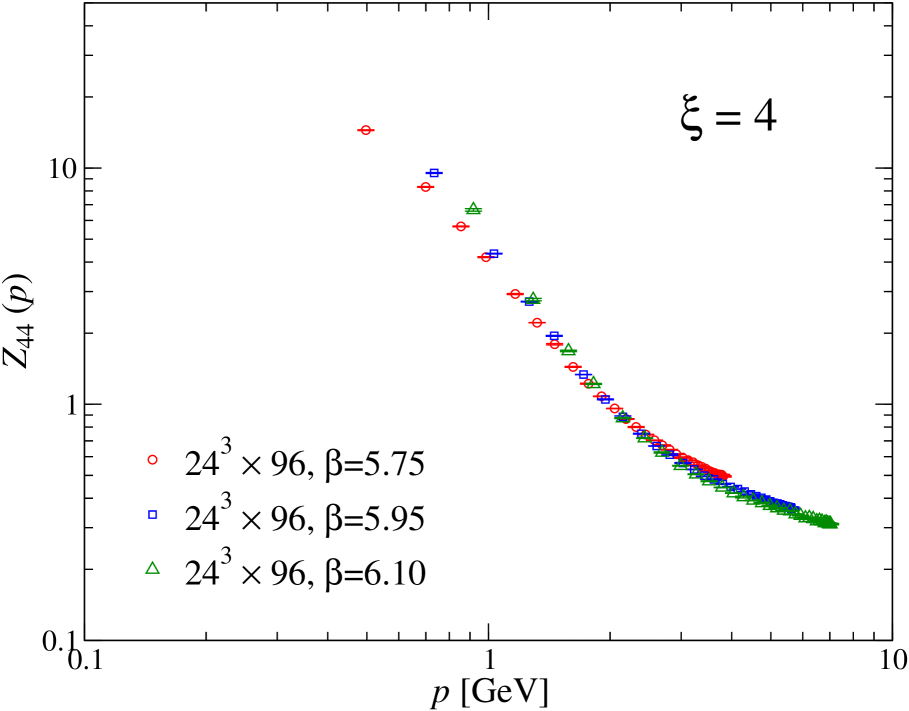
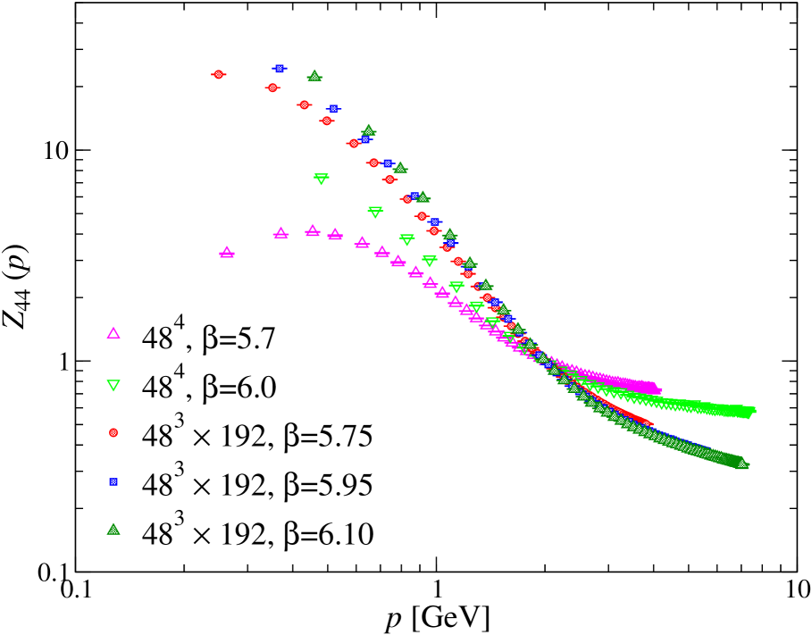
Figure 6: The dressing function of the instantaneous temporal gluon propagator on the isotropic lattice (top left), on the anisotropic lattice with $\xi=2$ (bottom left), and that with $\xi=4$ (top right). The results for the isotropic lattice and the anisotropic lattice with $\xi=4$ on the large lattice volume are drawn together in one figure for direct comparison (bottom right). The dressing function is renormalized to unity at $\lvert\vec{p}\rvert=2$ [GeV].

We next discuss the instantaneous temporal gluon propagator, which is related to the color-Coulomb potential. The dressing function of the time-time component of the gluon propagator is shown in Fig. 6 for the isotropic lattice and the anisotropic lattices. On the anisotropic lattices, the dressing function shows much better scaling behavior than that on the isotropic lattice. Although the small deviation can be seen both in the IR and UV region, one can expect that the scaling behavior is completely recovered in the Hamiltonian limit.

Moreover, we find that the IR behavior of $Z_{44}$ on the anisotropic lattice is different from that on the isotropic lattice (see bottom right panel). For the isotropic case, we see that the dressing function increases slowly with decreasing the momentum, and bends down on coarse lattice. By contrast, $Z_{44}$ continues to rise on the anisotropic lattice even for the coarsest lattice data ($\beta=5.75$), and $Z_{44}$ at available smallest momentum for the anisotropic case is about 10 times larger than that for the isotropic case. We note that the spatial lattice spacing for $(\xi,\beta)=(4,5.75)$ is larger than that for $(\xi,\beta)=(1,5.70)$. This implies that $Z_{44}$ is very sensitive to the discretization effects, and taking the Hamiltonian limit is crucial to cure scaling violation for the temporal gluon propagator and to explore the genuine IR divergent behavior in the Coulomb gauge QCD.

IX Power law fitting of $Z_{44}$ at small and large momenta

The asymptotic form of the color-Coulomb potential, the instantaneous part of the temporal gluon propagator, is given by

$$\lvert\vec{p}\rvert^{2}V_{44}(\lvert\vec{p}\rvert)\sim\frac{x_{0}}{2b_{0}\ln\left(\lvert\vec{p}\rvert/\Lambda_{\rm Coul}\right)},$$ (24)

where $x_{0}=12/11$ and $b_{0}=11/16\pi^{2}$ for SU(3) pure Yang-Mills theory, and $\Lambda_{\rm Coul}$ is a finite QCD mass scale Cucchieri and Zwanziger (2001b). We here fit the data for $Z_{44}$ with

$$Z_{44}(\lvert\vec{p}\rvert)=Z\frac{x_{0}}{2b_{0}\ln\left(\lvert\vec{p}\rvert/\Lambda_{\rm Coul}\right)}$$ (25)

in the momentum range $\lvert\vec{p}\rvert>6$ [GeV]. The fitted parameters $Z$ and $\Lambda_{\rm Coul}$ are given in Table 4 with $\chi^{2}/N_{DF}$. We find that the fitted parameter $\Lambda_{\rm Coul}$ takes an unacceptably small value as a QCD mass scale, although the $\chi^{2}$ value is reasonable for the isotropic lattice. $\Lambda_{\rm Coul}$ increases with the anisotropy and the fitted value $\Lambda_{\rm Coul}=0.8345(85)$ [GeV] for $\xi=4$ is the order of $\Lambda_{\rm QCD}$. However, the numerical data for the $\Lambda_{\rm QCD}$ parameter are still unstable under the increase of the anisotropy and $\Lambda_{\rm QCD}$ could change by further varying $\xi$. It can be stated that the anisotropy should be greater than $4$ otherwise we have physically inadequate results, although it is difficult to estimate the Hamiltonian limit of $\Lambda_{\rm QCD}$.

Table 4: The result of the UV logarithmic law fitting of $Z_{44}$ in the momentum range $\lvert\vec{p}\rvert\geq 6$ [GeV].

$(L_{\sigma}^{3}\times L_{\tau},\xi,\beta)$	$Z$	$\Lambda_{\rm Coul}$ [GeV]	$\chi^{2}/N_{\rm DF}$
(244, 1, 6.0)	0.648(97)	0.000968(1282)	0.406
(24${}^{3}\times$ 48, 2, 6.1)	0.310(80)	0.0385(507)	1.20
(24${}^{3}\times$ 96, 4, 6.1)	0.0842(41)	0.845(85)	2.22

In the IR region, the color-Coulomb potential is expected to behave as $1/\lvert\vec{p}\rvert^{2}$, which gives a linearly rising potential in position space. Indeed, the lattice simulations of the color-Coulomb potential obtained from the correlator of the partial Polyakov line revealed such a linearity of the color-Coulomb potential at large distances Greensite and Olejnik (2003); Nakamura and Saito (2006). Therefore, we fit the dressing function $Z_{44}$ with the power law form,

$$Z_{44}(\lvert\vec{p}\rvert)=\frac{z}{\lvert\vec{p}\rvert^{\gamma_{44}}}.$$ (26)

Assuming that the contribution of the vacuum polarization term to the instantaneous temporal gluon propagator is negligible, we expect $\gamma_{44}=2$ giving a linearly rising color-Coulomb potential.

The fitted results are given in Table 5. We observe that $\chi^{2}$ is extraordinary large and the fitting does not work. Even though the scaling violation becomes moderate as the anisotropy increases, we still have discretization effects which are visible in Fig. 6; the curves associated with different lattice couplings deviate from each other in the IR region and the slope gets steeper as the lattice spacing decreases. Therefore, we are still not close to the Hamiltonian limit where the scaling behavior is observed, and we cannot extract the color-Coulomb string tension from $Z_{44}(\lvert\vec{p}\rvert)$ and compare it with that obtained from the link-link correlator.

Table 5: The result of the IR power law fitting of $Z_{44}$. $\lvert\vec{p}_{max}\rvert$ represents the maximum momentum of the fitting range.

$(L_{\sigma},L_{\tau},\xi,\beta)$	$\lvert\vec{p}_{max}\rvert$	$z$	$\gamma_{44}$	$\chi^{2}/N_{\rm DF}$
( 48, 48, 1, 6.0 )	0.90	3.08(1)	1.22(1)	265
( 48, 192, 4, 6.1 )	0.90	5.42(2)	1.84(1)	248

X Instantaneous $D_{44}$ in position space and the color-Coulomb potential

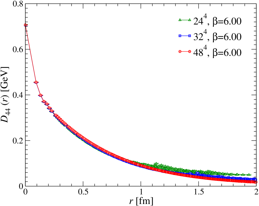
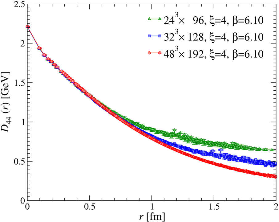
Figure 7: The instantaneous temporal gluon propagator in position space on the isotropic lattice (left) and the $\xi=4$ anisotropic lattice (right).

Since the instantaneous part of the temporal gluon propagator corresponds to the color-Coulomb potential,

$$D_{44}(\vec{x},t)=V_{c}(\vec{x})\delta(t)+P(\vec{x},t),$$ (27)

the color-Coulomb potential in the color-singlet channel is given by measuring the instantaneous $D_{44}$ in position space,

$$V^{\rm singlet}_{c}(\vec{x})=-\frac{4}{3}a_{\tau}D_{44}(\vec{x}).$$ (28)

Here the factor $-4/3$ is the Casimir invariant in the fundamental representation in the SU(3) gauge group. The instantaneous temporal gluon propagator in position space is drawn in Fig. 7 for the isotropic and the $\xi=4$ anisotropic lattices. We observe that the behavior of $D_{44}$ notably changes by increasing the anisotropy. $D_{44}$ decreases almost linearly with distance in the range $3\leq r\leq 7$ [fm] for the anisotropic lattice while it does not on the isotropic lattice. The linear decrease of $D_{44}$ means that $V_{c}$ is a linearly rising potential with distance, which is consistent with the lattice calculations of $V_{c}$ from the correlator of the partial Polyakov line. On the isotropic lattice, there are unavoidable contributions from the polarization term in the instantaneous propagator on the lattice, and it is indispensable to carry out the lattice simulations with small temporal spacing to extract $V_{c}$ from the instantaneous $D_{44}$.

We fit the data with the function

$$V^{\rm singlet}_{c}(r)=C+\sigma_{c}r,$$ (29)

in the range $0.4\leq r\leq 0.7$ [fm] and extract the color-Coulomb string tension $\sigma_{c}$. The fitted result is given in Table 6. We see that the fitting is extremely worse for the isotropic lattice, and $\chi^{2}/N_{\rm DF}$ approaches $O(1)$ on the anisotropic lattice. Besides a large $\chi^{2}$ value, the color-Coulomb string tension on the isotropic lattice is smaller than the Wilson string tension violating the Zwanziger’s inequality Zwanziger (2003). The extracted $\sigma_{c}$ increases with decreasing the temporal lattice spacing and satisfies the Zwanziger’s inequality on the finer lattices. Although $\sigma_{c}$ from the instantaneous $D_{44}$ is still smaller than that from the correlator of the partial Polyakov loop, there is little doubt that $\sigma_{c}$ does not saturate the Zwanziger’s inequality and $\sigma_{c}$ is larger than the string tension of the Wilson static potential.

It may be surprising that we can extract $\sigma_{c}$ with reasonable $\chi^{2}$ values on finer anisotropic lattices. We have seen in the last section that the power law fitting of $Z_{44}$ does not work, even though the extracted value of $\gamma_{44}$ is close to 2, which gives a linearly rising color-Coulomb potential. On the anisotropic lattice, the largest lattice volume is $4.67^{4}$ [fm⁴] (circles in the right panel of Fig. 7) and we naively expect that the finite volume effects on the instantaneous $D_{44}$ are not so serious in the range $r\leq 2$ [fm]. However, Fig. 7 shows that $D_{44}$ does not show a linearly decreasing behavior at $r\geq 1$ [fm]. This indicates that we still need to approach the Hamiltonian limit to extract the color-Coulomb potential from the instantaneous temporal gluon propagator and to compare the color-Coulomb string tension with that from the correlator of the partial Polyakov loop.

Table 6: The result of the fitting of $V_{c}$ in the range $0.4\leq r\leq 0.7$ [fm].

$(L_{\sigma},L_{\tau},\xi,\beta)$	$C$ [GeV]	$\sqrt{\sigma}$ [MeV]	$\chi^{2}/N_{\rm DF}$
(48, 48, 1, 6.00)	-0.4971(4)	289.9(3)	39.1
(48, 192, 4, 5.75)	-1.262(2)	423.2(9)	11.3
(48, 192, 4, 5.95)	-1.995(5)	515.7(18)	1.26
(48, 192, 4, 6.10)	-2.634(5)	580.0(16)	0.828

XI Conclusions

It is a central interest to explore the IR behavior of the gluon propagator to reveal the confinement mechanism in QCD. In the Coulomb gauge, the instantaneous gluon propagator suffers from significant discretization errors on isotropic lattices. In this paper, we calculated the transverse and the temporal components of the instantaneous gluon propagator on isotropic and anisotropic lattices and studied the scaling behavior.

We find that the transverse gluon propagator shows a nice scaling behavior on the anisotropic lattices, and scaling violation observed on the isotropic lattice almost disappear on $\xi=4$ anisotropic lattice. It is natural to expect that the perfect scaling behavior can be seen and the multiplicative renormalizability holds in the Hamiltonian limit $a_{\tau}\to 0$. In the IR region, the transverse gluon propagator is strongly suppressed on both the isotropic and the anisotropic lattices and shows the turnover at about 500 [MeV] in both cases.

We also calculated the transverse gluon propagator in position space, and it shows that the correlation function quickly decreases at small distances and becomes negative in the range $r\sim 1-2$ [fm], and vanishes at large distances. This means that the gluon fields have no correlation beyond the hadronic scale, and it is consistent with the fact that the gluons are confined in the hadrons (glueballs).

The power law fitting of the transverse gluon propagator exhibits that the UV exponent $\gamma_{\rm gl}^{\rm UV}$ decreases with increasing the anisotropy. This supports the expectation that the gluons behave as free massless particles at sufficiently large momentum in the continuum due to asymptotic freedom.

In order to explore the IR behavior of the transverse gluon propagator, we fitted the data with the power law and found that the extracted value of the IR exponent is positive on the isotropic and anisotropic lattices. However, our lattice is still small to extract a reliable value of the IR exponent on the anisotropic lattices. Fitting the transverse gluon propagator with the Gribov-type ansatz did not work in our lattice data, which successfully describe the SU(2) lattice data employing different method to cure scaling violation Burgio et al. (2009), and it deserves further study whether this is due to the difference of the gauge group or the adopted prescriptions to remedy scaling violation.

For the temporal gluon propagator, scaling violation was observed both in the IR and UV regions on the isotropic lattice in contrast to the transverse propagator, for which lattice data do not suffer from discretization errors in the IR region. Our results show that the lattice data on the anisotropic lattices show much better scaling behavior than that on the isotropic lattice, although the discretization errors are still seen in the IR and the UV regions.

We observed that the time-time gluon propagator on the anisotropic lattice is much more enhanced in the IR region compared to that on the isotropic lattice. The turnover observed on the coarsest lattice data on isotropic lattice disappears on the finer lattices, and $Z_{44}$ monotonically increases with decreasing the momentum on $\xi=4$ anisotropic lattice. However, the IR power law fitting did not work for the dressing function, although the fitted value $\gamma_{44}$=1.84(1) on the finest lattice is close to the expected value for the linearly rising behavior of the color-Coulomb potential. We again need larger lattices as the transverse gluon propagator.

The logarithmic law fitting of the dressing function of the temporal propagator in the UV region indicates that the extracted $\Lambda_{\rm Coul}$ is unacceptably small on the isotropic lattice and it takes 0.845(85) [GeV] on the finest anisotropic lattice, which is the order of $\Lambda_{\rm QCD}$.

In position space, the linearly decreasing behavior can be seen on the anisotropic lattice, and the color-Coulomb string tension obeys the Zwanziger’s inequality on finer anisotropic lattices. However, the extracted value is still smaller than that obtained from the correlator of the partial Polyakov line. Thus, we can say that although the scaling violation is softened by decreasing the temporal lattice spacing, the instantaneous temporal gluon propagator receives a contribution from the polarization term and it is difficult to extract the color-Coulomb potential from the instantaneous $D_{44}$ for finite $a_{\tau}$.

Appendix A Tolerance of the gauge fixing and the IR suppression of $D^{\rm tr}$

The tolerance of the gauge fixing is crucial for the IR suppression of the instantaneous transverse gluon propagator. In the iterative gauge fixing on the lattice, we stop the gauge transformation if the violation of the transversality becomes less than some small number $\epsilon$;

$$\theta=\frac{1}{(N_{c}^{2}-1)L_{\sigma}^{3}}\sum_{\vec{x},a,i}(\nabla_{i}A_{i}^{\rm lat}(\vec{x},t))^{2}<\epsilon.$$ (30)

We set $\epsilon=10^{-14}$ in our calculations. In this appendix, we examine the behavior of the instantaneous transverse gluon propagator by varying $\epsilon$ on the isotropic lattice.

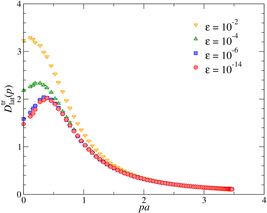
Figure 8: The instantaneous transverse gluon propagator in lattice units on $56^{4}$ lattice at $\beta=5.7$ for various $\epsilon$. The cylinder cut is applied, but the cone cut is not.

Figure 8 shows $D^{\rm tr}(\vec{p})$ in lattice units on $56^{4}$ lattice at $\beta=5.7$ for various $\epsilon$. For all the cases, the measurements are done for 20 configurations and the cylinder cut is applied. We observe that the propagator does not exhibit a turnover for $\epsilon=10^{-2}$ and the curve deviates from that for $\epsilon=10^{-14}$ in the region $pa\leq 1.5$. Decreasing $\epsilon$ by the factor 100 diminishes the propagator at small momenta and $D^{\rm tr}$ coincides within the statistical errors in the range $1\leq pa$. A further decrease of $\epsilon$ suppresses $D^{\rm tr}$ in the IR region and the transverse propagator shows a clear turnover. Although the data for $\epsilon=10^{-8}$ are not depicted in Fig. 8, they fall on top of the data for $\epsilon=10^{-14}$ within the error bars. Therefore, $\epsilon$ should be sufficiently small to explore the IR behavior of the gluon propagator and $10^{-14}$ is small enough.

Appendix B Scaling violation in the free field case

In this appendix, we discuss scaling violation of the instantaneous propagator in the free field case. A more general case was discussed in LABEL:Burgio:2008jr.

The instantaneous transverse propagator in the continuum is given by integrating the unequal-time propagator over $p_{4}$,

$$D(\vec{p})=\int^{\infty}_{-\infty}\frac{dp_{4}}{2\pi}D(\vec{p},p_{4}).$$ (31)

In the free field case (i.e., at the zeroth order in the coupling), the four-dimensional propagator is $D_{\rm{free}}(\vec{p},p_{4})=1/(\lvert\vec{p}\rvert^{2}+p_{4}^{2})$ and the instantaneous propagator is

$$D_{\rm{free}}(\vec{p}) = \int^{\infty}_{-\infty}\frac{dp_{4}}{2\pi}\frac{1}{\lvert\vec{p}\rvert^{2}+p_{4}^{2}}$$ (32)

$$= \left.\frac{1}{2\pi\lvert\vec{p}\rvert}\arctan\left(\frac{p_{4}}{\lvert\vec{p}\rvert}\right)\right|^{p_{4}=\infty}_{p_{4}=-\infty}$$

$$= \frac{1}{2\lvert\vec{p}\rvert}.$$

On a lattice with a finite temporal spacing $a_{\tau}$, the $p_{4}$ integral is limited within the range $-\pi/a_{\tau}\leq p_{4}\leq\pi/a_{\tau}$. Thus, the instantaneous propagator is given by

$$D_{\rm{free}}(\vec{p},a_{\tau}) = \int^{\pi/a_{\tau}}_{-\pi/a_{\tau}}\frac{dp_{4}}{2\pi}\frac{1}{\lvert\vec{p}\rvert^{2}+p_{4}^{2}}$$ (33)

$$= \left.\frac{1}{2\pi\lvert\vec{p}\rvert}\arctan\left(\frac{p_{4}}{\lvert\vec{p}\rvert}\right)\right|^{p_{4}=\pi/a_{\tau}}_{p_{4}=-\pi/a_{\tau}}$$

$$= \frac{1}{2\lvert\vec{p}\rvert}\frac{2}{\pi}\arctan\left(\frac{\pi}{a_{\tau}\lvert\vec{p}\rvert}\right).$$

For a finite temporal lattice spacing, we have an extra factor

$$\frac{2}{\pi}\arctan\left(\frac{\pi\xi}{\hat{p}}\right),$$ (34)

where $\hat{p}=\lvert\vec{p}\rvert a_{\sigma}$ is the spatial momentum in lattice units, and $\xi$ is the anisotropy, $\xi=a_{\sigma}/a_{\tau}$. This extra factor approaches unity in the Hamiltonian limit $a_{\tau}\to 0$.

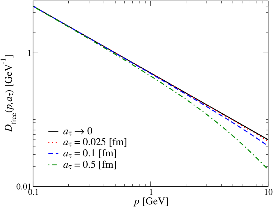
Figure 9: $D_{\rm{free}}(\lvert\vec{p}\rvert,a_{\tau})$ is plotted as a function of $p$ for various temporal lattice spacings.

The free instantaneous propagator for various temporal lattice spacings is illustrated in Fig. 9. We observe that the propagator starts to deviate from that in the Hamiltonian limit at larger momenta as $a_{\tau}$ decreases. Accordingly, scaling violation is observed even in the free field case and it goes away in the Hamiltonian limit. If we impose some renormalization condition, $D_{\rm free}(\lvert\vec{p}\rvert=1{\rm[GeV]})=1$ [GeV^-1] for instance, the curves in Fig. 9 cross at the renormalization point and deviate from each other in both the small and the large momentum regions, which is the situation we encountered in the lattice simulations. From this simple exercise, we expect that scaling violation for the instantaneous gluon propagator would be moderate for small temporal lattice spacing.

References

- Zwanziger (1994) D. Zwanziger, Nucl. Phys. B412, 657 (1994).
- Greensite et al. (2005) J. Greensite, S. Olejnik, and D. Zwanziger, JHEP 05, 070 (2005), eprint hep-lat/0407032.
- Nakagawa et al. (2007) Y. Nakagawa, A. Nakamura, T. Saito, and H. Toki, Phys. Rev. D75, 014508 (2007), eprint hep-lat/0702002.
- Greensite and Olejnik (2003) J. Greensite and S. Olejnik, Phys. Rev. D67, 094503 (2003), eprint hep-lat/0302018.
- Nakamura and Saito (2006) A. Nakamura and T. Saito, Prog. Theor. Phys. 115, 189 (2006), eprint hep-lat/0512042.
- Nakagawa et al. (2006) Y. Nakagawa, A. Nakamura, T. Saito, H. Toki, and D. Zwanziger, Phys. Rev. D73, 094504 (2006), eprint hep-lat/0603010.
- Nakagawa et al. (2008) Y. Nakagawa, A. Nakamura, T. Saito, and H. Toki, Phys. Rev. D77, 034015 (2008), eprint arXiv:0802.0239.
- Zwanziger (2003) D. Zwanziger, Phys. Rev. Lett. 90, 102001 (2003), eprint hep-lat/0209105.
- Voigt et al. (2008) A. Voigt, E. M. Ilgenfritz, M. Muller-Preussker, and A. Sternbeck, Phys. Rev. D78, 014501 (2008), eprint arXiv:0803.2307.
- Zwanziger (1991) D. Zwanziger, Nucl. Phys. B364, 127 (1991).
- Bogolubsky et al. (2009) I. L. Bogolubsky, E. M. Ilgenfritz, M. Muller-Preussker, and A. Sternbeck, Phys. Lett. B676, 69 (2009), eprint arXiv:0901.0736.
- Fischer et al. (2009) C. S. Fischer, A. Maas, and J. M. Pawlowski, Annals Phys. 324, 2408 (2009), eprint arXiv:0810.1987.
- Cucchieri and Zwanziger (2001a) A. Cucchieri and D. Zwanziger, Phys. Rev. D65, 014001 (2001a), eprint hep-lat/0008026.
- Langfeld and Moyaerts (2004) K. Langfeld and L. Moyaerts, Phys. Rev. D70, 074507 (2004), eprint hep-lat/0406024.
- Burgio et al. (2009) G. Burgio, M. Quandt, and H. Reinhardt, Phys. Rev. Lett. 102, 032002 (2009), eprint arXiv:0807.3291.
- Nakagawa et al. (2009) Y. Nakagawa et al., Phys. Rev. D79, 114504 (2009), eprint arXiv:0902.4321.
- Szczepaniak and Swanson (2001) A. P. Szczepaniak and E. S. Swanson, Phys. Rev. D65, 025012 (2001), eprint hep-ph/0107078.
- Szczepaniak (2004) A. P. Szczepaniak, Phys. Rev. D69, 074031 (2004), eprint hep-ph/0306030.
- Feuchter and Reinhardt (2004) C. Feuchter and H. Reinhardt, Phys. Rev. D70, 105021 (2004), eprint hep-th/0408236.
- Epple et al. (2007) D. Epple, H. Reinhardt, and W. Schleifenbaum, Phys. Rev. D75, 045011 (2007), eprint hep-th/0612241.
- Epple et al. (2008) D. Epple, H. Reinhardt, W. Schleifenbaum, and A. P. Szczepaniak, Phys. Rev. D77, 085007 (2008), eprint arXiv:0712.3694.
- Campagnari and Reinhardt (2008) D. R. Campagnari and H. Reinhardt, Phys. Rev. D78, 085001 (2008), eprint arXiv:0807.1195.
- Watson and Reinhardt (2008) P. Watson and H. Reinhardt, Phys. Rev. D77, 025030 (2008), eprint arXiv:0709.3963.
- Reinhardt and Watson (2009) H. Reinhardt and P. Watson, Phys. Rev. D79, 045013 (2009), eprint arXiv:0808.2436.
- Watson and Reinhardt (2009) P. Watson and H. Reinhardt, Eur. Phys. J. C65, 567 (2009), eprint arXiv:0812.1989.
- Burgio et al. (2010) G. Burgio, M. Quandt, and H. Reinhardt, Phys.Rev. D81, 074502 (2010), eprint arXiv:0911.5101.
- Quandt et al. (2008) M. Quandt, G. Burgio, S. Chimchinda, and H. Reinhardt, PoS CONFINEMENT8, 066 (2008), eprint arXiv:0812.3842.
- Leinweber et al. (1999) D. B. Leinweber, J. I. Skullerud, A. G. Williams, and C. Parrinello, Phys. Rev. D60, 094507 (1999), eprint hep-lat/9811027.
- Cucchieri and Zwanziger (2001b) A. Cucchieri and D. Zwanziger, Phys. Rev. D65, 014002 (2001b), eprint hep-th/0008248.
- Zwanziger (1998) D. Zwanziger, Nucl. Phys. B518, 237 (1998).
- Klassen (1998) T. R. Klassen, Nucl. Phys. B533, 557 (1998), eprint hep-lat/9803010.
- Namekawa et al. (2001) Y. Namekawa et al. (CP-PACS), Phys. Rev. D64, 074507 (2001), eprint hep-lat/0105012.
- Matsufuru et al. (2001) H. Matsufuru, T. Onogi, and T. Umeda, Phys. Rev. D64, 114503 (2001), eprint hep-lat/0107001.
- Necco and Sommer (2002) S. Necco and R. Sommer, Nucl. Phys. B622, 328 (2002), eprint hep-lat/0108008.
- Davies et al. (1988) C. T. H. Davies et al., Phys. Rev. D37, 1581 (1988).