Partitioning technique for a discrete quantum system

Abstract

We develop the partitioning technique for quantum discrete systems. The graph consists of several subgraphs: a central graph and several branch graphs, with each branch graph being rooted by an individual node on the central one. We show that the effective Hamiltonian on the central graph can be constructed by adding additional potentials on the branch-root nodes, which generates the same result as does the the original Hamiltonian on the entire graph. Exactly solvable models are presented to demonstrate the main points of this paper.

I Introduction

The Schrödinger equation lies at the heart of quantum mechanics. Secular equation has analytic solutions only for a few very special cases. Approximation techniques and computational methods have been developed for treating such problem. Many of them are rooted in the partitioning technique Lindgren ; Hubac which was introduced by Feshbach Feshbach and Löwdin Lowdin independently. Discrete models, including quantum networks, have been a cornerstone of theoretical explorations due to their analytical and numerical tractability WXG , the availability of exact solutions, and the ability to capture counter-intuitive physical phenomena, such as non-spreading wavepacket Kim and Bloch oscillation FBloch ; CZener ; Hartmann in linear chain. In recent years, optical lattice IBloch ; Zoller , photonic crystal KML ; UG , etc. have increasingly permitted the experimental exploration of quantum discrete models.

In this paper, we study the partitioning technique for quantum discrete systems. The concerned graph consists of several subgraphs: a central graph and several branch graphs, with each branch graph being rooted by an individual node on the central one. Applying the projection theory Lowdin to such a graph, we show that the effective Hamiltonian on the central graph can be constructed by adding additional potentials on the branch-root nodes, which generates the same result as does the the original Hamiltonian on the entire graph. As the demonstration, we present two exactly solvable models, which correspond to real and imaginary potentials.

This paper is organized as follows. Section II shows a formalism for the partitioning technique in discrete quantum systems. Section III is the heart of this paper which presents a method to obtain the projection Hamiltonian. Section IV consists of two exactly solvable examples to illustrate our main idea. Section V is the summary and discussion.

II Partitioning technique

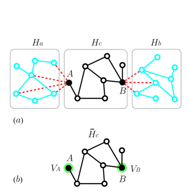
Figure 1: (Color online)(a) Schematic illustration of the graph consisted of two branch graphs $a$, $b$ (cyan) and a center graph $c$ (black). The dashed edges (red) represent the connections between them with $A$ and $B$ being the branch-root nodes. (b) The Löwdin’s projection Hamiltonian for the center graph which is composed of the original Hamiltonian $H_{c}$ and additional on-site potentials $V_{A}$ and $V_{B}$ on the nodes $A$ and $B$, respectively.

Löwdin has developed a partitioning technique in the algebra of matrices, with which various self-consistent field methods can be nicely formulated. In this procedure, the original Hamiltonian is simply transformed in a chosen discrete representation. The entire space is usually divided into two subspaces, named a model space and an orthogonal space. The basic idea is to find an effective Hamiltonian which acts only within the target model space but generates the same result as the original Hamiltonian acting on the complete space Lindgren ; Hubac . The partitioning technique enables us focus our interest on certain part of the system. In general, the effective Hamiltonian cannot be obtained explicitly, but provides a formalism to develop perturbation method.

In the following we will show that, when the technique is applied to a specific discrete system, the effective Hamiltonian is of realistic significance. We consider a quantum graph, which is a collection of nodes and edges. It is also equivalent to a single-particle tight-binding model. For simplicity, we partition the complete graph into three subgraphs, a central part $c$, two independent branches $a$ and $b$.

The Hamiltonian (or connectivity matrix) of such a graph has the form

$$H=\left(\begin{array}[]{ccc}H_{a}&H_{ac}&0\\ H_{ca}&H_{c}&H_{cb}\\ 0&H_{bc}&H_{b}\end{array}\right),$$ (1)

where

$$H_{a} = -\sum_{i,j=1}^{N_{a}}\left(\kappa_{ij}^{a}\left|i\right\rangle_{a}\left\langle j\right|+\text{H.c.}\right),$$ (2)

$$H_{b} = -\sum_{i,j=1}^{N_{b}}\left(\kappa_{ij}^{b}\left|i\right\rangle_{b}\left\langle j\right|+\text{H.c.}\right),$$ (3)

$$H_{c} = -\sum_{i,j=1}^{N_{c}}\left(\kappa_{ij}^{c}\left|i\right\rangle_{c}\left\langle j\right|+\text{H.c.}\right),$$ (4)

Here $N_{\gamma=a,b,c}$ denotes the dimension of the three subgraphs. $\kappa_{ij}^{\gamma=a,b,c}$ denotes the coupling between $i$ and $j$ of the graph $\gamma$, and reduces to the on-site potential for $i=j$. The connections between the subgraphs are

$$H_{ca} = H_{ac}^{\dagger}=-\sum_{i=1}^{N_{c}}\sum_{j=1}^{N_{a}}g_{ij}^{a}\left|i\right\rangle_{ca}\left\langle j\right|,$$ (5)

$$H_{cb} = H_{bc}^{\dagger}=-\sum_{i=1}^{N_{c}}\sum_{j=1}^{N_{b}}g_{ij}^{b}\left|i\right\rangle_{cb}\left\langle j\right|.$$ (6)

where $g_{ij}^{\gamma=a,b}$ is the coupling strength between $\left|j\right\rangle_{\gamma}$ and branch-root nodes $\left|i\right\rangle_{c}$.

Our aim is the solution of the Schrödinger equation

$$H\left|f_{k}\right\rangle=E_{k}\left|f_{k}\right\rangle,$$ (7)

where

$$\left|f_{k}\right\rangle=\sum_{\gamma=a,b,c}\sum_{l=1}^{N_{\gamma}}f_{k}^{\gamma}\left(l\right)\left|l\right\rangle_{\gamma}.$$ (8)

Then the Schrödinger equation can be written in the matrix form

$$\left(\begin{array}[]{ccc}H_{a}&H_{ac}&0\\ H_{ca}&H_{c}&H_{cb}\\ 0&H_{bc}&H_{b}\end{array}\right)\left(\begin{array}[]{c}f_{k}^{a}\\ f_{k}^{c}\\ f_{k}^{b}\end{array}\right)=E_{k}\left(\begin{array}[]{c}f_{k}^{a}\\ f_{k}^{c}\\ f_{k}^{b}\end{array}\right),$$ (9)

and more explicit form

$$H_{a}f_{k}^{a}+H_{ac}f_{k}^{c} = E_{k}f_{k}^{a},$$ (10)

$$H_{c}f_{k}^{c}+H_{ca}f_{k}^{a}+H_{cb}f_{k}^{b} = E_{k}f_{k}^{c},$$ (11)

$$H_{b}f_{k}^{b}+H_{bc}f_{k}^{c} = E_{k}f_{k}^{b}.$$ (12)

Under the condition of the existence of the inverse matrices $\left(E_{k}-H_{a}\right)^{-1}$ and $\left(E_{k}-H_{b}\right)^{-1}$, we have

$$f_{k}^{a} = \left(E_{k}-H_{a}\right)^{-1}H_{ac}f_{k}^{c},$$ (13)

$$f_{k}^{b} = \left(E_{k}-H_{b}\right)^{-1}H_{bc}f_{k}^{c},$$ (14)

Then the Löwdin’s projection Hamiltonian $\bar{H}_{c}$ has the form

$$\bar{H}_{c}=H_{c}+\bar{H}_{a}+\bar{H}_{b},$$ (15)

where

$$\bar{H}_{a} = H_{ca}\left(E_{k}-H_{a}\right)^{-1}H_{ac},$$ (16)

$$\bar{H}_{b} = H_{cb}\left(E_{k}-H_{b}\right)^{-1}H_{bc}.$$ (17)

Remarkably, the corresponding Schrödinger equation for the subgraph $c$ (Eq. (11)) is reduced to

$$\bar{H}_{c}f_{k}^{c}=E_{k}f_{k}^{c},$$ (18)

i.e., formally $\bar{H}_{c}$ can lead the same result as the original Hamiltonian acted with respect to the whole graph, then is referred as the effective Hamiltonian for central graph. Nevertheless, in general, one cannot treat Eq. (18) as usual since it is hard to obtain the explicit matrix form of $\bar{H}_{c}$.

III Effective Hamiltonian for central graph

It can be seen from Eq. (15) that, $\bar{H}_{c}$ is constructed based on the original subgraph $H_{c}$. It indicates that the impact of two branch graphs can be projected on the target graph as additional couplings or on-site potentials. In this paper, we investigate a graph with each independent branch graph connected to the central graph $c$ via a single node on the central graph. This is crucial and our conclusion is available for a graph with arbitrary branches. In the following we will show that $\bar{H}_{a}$ and $\bar{H}_{b}$ have a concise form and clear physical meaning.

The connections between the subgraphs are

$$H_{ca} = H_{ac}^{\dagger}=-\sum_{j}^{N_{a}}g_{j}^{a}\left|A\right\rangle_{ca}\left\langle j\right|,$$ (19)

$$H_{cb} = H_{bc}^{\dagger}=-\sum_{j}^{N_{b}}g_{j}^{b}\left|B\right\rangle_{cb}\left\langle j\right|.$$ (20)

Note that there is only one branch-root node for each branch, that is the unique restriction to the graph.

We note from Eq. (19) that the elements of $H_{ca}$ and $H_{ac}^{{\dagger}}$ are all zeros except the row connecting to node $A$, i.e.,

$$H_{ca}\left(m,n\right)=\delta_{mA}g_{n}^{a},\text{ }H_{ac}\left(m,n\right)=\delta_{nA}\left(g_{m}^{a}\right)^{\ast}.$$ (21)

Taking $M^{a}=\left(E_{k}-H_{a}\right)^{-1}$ and assuming its existence for the considering eigenvalue $E_{k}$, we have

$$\bar{H}_{a}\left(m,n\right) = \sum_{j^{\prime}=1}^{N_{a}}[\sum_{j=1}^{N_{a}}H_{ca}\left(m,j\right)M^{a}\left(j,j^{\prime}\right)]H_{ac}\left(j^{\prime},n\right)$$ (22)

$$= \sum_{j^{\prime}=1}^{N_{a}}[\sum_{j=1}^{N_{a}}\delta_{mA}g_{j}^{a}M^{a}\left(j,j^{\prime}\right)]\delta_{nA}(g_{j^{\prime}}^{a})^{\ast}$$

$$= \delta_{mA}\delta_{nA}\sum_{j,j^{\prime}=1}^{N_{a}}g_{j}^{a}(g_{j^{\prime}}^{a})^{\ast}M^{a}\left(j,j^{\prime}\right).$$

Moreover, from Eqs. (13) and (16) we obtain

$$H_{ca}f_{k}^{a}=\bar{H}_{a}f_{k}^{c}$$ (23)

and its explicit form

$$\sum_{j=1}^{N_{a}}g_{j}^{a}f_{k}^{a}\left(j\right)=f_{k}^{c}\left(A\right)\sum_{j,j^{\prime}=1}^{N_{a}}g_{j}^{a}(g_{j^{\prime}}^{a})^{\ast}M^{a}\left(j,j^{\prime}\right).$$ (24)

Considering the non-trivial case $f_{k}^{c}\left(A\right)\neq 0$, the effective Hamiltonian $\bar{H}_{a}$ can be expressed as

$$\bar{H}_{a}\left(m,n\right)=\frac{\delta_{mA}\delta_{nA}}{f_{k}^{c}\left(A\right)}\sum_{j=1}^{N_{a}}g_{j}^{a}f_{k}^{a}\left(j\right).$$ (25)

By a similar procedure we obtain expression for the effective Hamiltonian $\bar{H}_{b}$

$$\bar{H}_{b}\left(m,n\right)=\frac{\delta_{mB}\delta_{nB}}{f_{k}^{c}\left(B\right)}\sum_{j=1}^{N_{b}}g_{j}^{b}f_{k}^{b}\left(j\right).$$ (26)

Surprisingly, matrix $\bar{H}_{a}$ ($\bar{H}_{b}$) contains only one nonzero element $\bar{H}_{a}(A,A)$ ($\bar{H}_{b}(B,B)$), which can be regarded as an effective on-site potential at the branch-root node $A$ ($B$). Actually, this is caused by the unique restriction. Then the physics of the projection Hamiltonian is very clear: original target Hamiltonian with additional potentials at the joint sites. The effective potential is a weighted summation of the coupling strength $\{g_{j}^{\gamma=a,b}\}$ and the corresponding amplitudes $\{f_{k}\left(j\right)\}$. It would be noted that this conclusion can be generalized into graphs with more independent branches $d,e,\cdots$.

One can simply classify the branch graph as finite or infinite. For finite graph without flux, we have $\{g_{j}^{\gamma=a,b,\cdots}\}$ and the corresponding $\left\{f_{k}\left(j\right)\right\}$ are all real, then the effective on-site potentials are real. In contrary, for an infinite graph, when dealing with the scattering problem, the effective on-site potentials could be complex.

IV ILLUSTRATIVE EXAMPLES

In this section, two typical examples, which consist of finite and infinite branch graphs, are respectively investigated to exemplify the formalism developed above.

IV.1 Finite chain

We first take a finite chain $N$ as an example, with the Hamiltonian in the form

$$H_{\text{Chain}}=-J\sum_{i=1}^{N-1}\left(\left|i\right\rangle\left\langle i+1\right|+\text{H.c.}\right).$$

It is well known that the eigenvalue $E_{k}$ and the corresponding eigenvector $f_{k}$ are

$$E_{k} = -2J\cos k,$$ (27)

$$f_{k}\left(j\right) = \sqrt{\frac{2}{N+1}}\sin\left(kj\right),$$ (28)

$$k = \frac{n\pi}{N+1},n\in[1,N].$$

Now we divide the chain $N$ as the central part $N_{c}$ and two branches $N_{a}$, $N_{b}$ as mentioned above. The two branch-root nodes are located at the $\left(N_{a}+1\right)$th and $\left(N_{a}+N_{c}\right)$th sites. From Eqs. (25) and (26), the projection Hamiltonian can be obtained as

$$\mathcal{\bar{H}}_{c} = -J\sum_{i=N_{a}+1}^{N_{a}+N_{c}-1}\left(\left|i\right\rangle\left\langle i+1\right|+\text{H.c.}\right)$$

$$+V_{A}\left|N_{a}+1\right\rangle\left\langle N_{a}+1\right|+V_{B}\left|N_{a}+N_{c}\right\rangle\left\langle N_{a}+N_{c}\right|,$$

where the on-site potentials are

$$V_{A} = -J\frac{\sin\left(kN_{a}\right)}{\sin\left[k\left(N_{a}+1\right)\right]},$$ (30)

$$V_{B} = -J\frac{\sin\left[k\left(N_{a}+N_{c}+1\right)\right]}{\sin\left[k\left(N_{a}+N_{c}\right)\right]}.$$ (31)

In the Appendix A.1, it is shown that $E_{k}$ is always the eigenvalue of $\mathcal{\bar{H}}_{c}$ and the corresponding eigenvector of $\mathcal{\bar{H}}_{c}$ accords with that of $H_{\text{Chain}}$ within the central chain $c$. It is noted that potential $V_{A}$ ($V_{B}$) does not exists in the case $\sin\left[k\left(N_{a}+1\right)\right]=0$ ($\sin\left[k\left(N_{a}+N_{c}\right)\right]=0$). Actually, the corresponding eigenfunction has vanishing amplitude at the node $A$ ($B$), and $E_{k}$ is also the eigenvalue of the branch Hamiltonian $H_{a}$ ($H_{b}$) simultaneously. From the viewpoint of the projection theory, the corresponding inverse matrix $\left(E_{k}-H_{a}\right)^{-1}$ or $\left(E_{k}-H_{b}\right)^{-1}$ does not exist.

Now we look at a concrete example in order to give a sense of the conclusion. Consider a $15$-site chain with $N_{a}=5$, $N_{c}=4$, and $N_{b}=6$. Taking $k=\pi/4$ as an example, the corresponding eigenvalue and eigenvector for the entire chain are $E_{\pi/4}=-\sqrt{2}J$, $f_{\pi/4}\left(j\right)$ $=\sqrt{2}/4\sin\left(j\pi/4\right)$, on the central chain $c$, $f_{\pi/4}^{c}$ $=-(\sqrt{2},1,0,-1)/4$. On the other hand, from Eqs. (27), (28), (30) and (31), we have $V_{A}$ $=-J\sin\left(5k\right)/\sin\left(6k\right)$ $=-\sqrt{2}/2J$ and $V_{B}$ $=-J\sin\left(10k\right)/\sin\left(9k\right)$ $=-\sqrt{2}J$. Then the corresponding effective Hamiltonian is

$$H_{c}^{\text{eff}}=-J\sum_{i=6}^{8}\left(\left|i\right\rangle\left\langle i+1\right|+\text{H.c.}\right)-J(\frac{\sqrt{2}}{2}\left|6\right\rangle\left\langle 6\right|+\sqrt{2}\left|9\right\rangle\left\langle 9\right|),$$ (32)

to solve $H_{c}^{\text{eff}}$, we use the formula Eq. (51) derived in the Appendix A.1. It becomes

$$\sin\left(4\kappa\right)(2\cos\kappa-\frac{3\sqrt{2}}{2})=0,$$ (33)

which has the solutions $E_{\kappa}=-2J\cos\kappa$ $=\sqrt{2}J$, $0$, $-\sqrt{2}J$, and $-3\sqrt{2}/2J$. The corresponding eigenvector for $E_{\kappa}=-\sqrt{2}J$ can be obtained as $(f_{\pi/4}^{\text{eff}})^{\dagger}\propto(\sqrt{2},1,0,-1)$, which accords with wavefunction of whole system within the chain $c$, $f_{\pi/4}^{c}$.

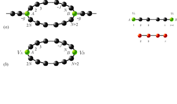
Figure 2: (Color online) Schematic illustration of the concrete configuration for a scattering system. A ring as the scattering center, connects to two semi-infinite chains $L$ and $R$ as waveguides with coupling $-g$. The wave function within the scattering center for a scattering state of the whole system is identical to an equal-energy eigen function of the projection Hamiltonian which is constructed by the center ring with additional on-site potentials $V_{A}$ and $V_{B}$ added at the joint sites $A$ and $B$.

IV.2 Scattering problem

In the above example, we can see that all the potentials are real. It was predicted that the infinite branches could induce the imaginary potentials. Here we are interested in the scattering solution of an infinite system. Quantum scattering and transport properties in quantum networks are important features in quantum information science Kim ; ZhouL ; JLTrans . Now we consider an exactly solvable but non-trivial system to illustrate the main idea of this paper.

The graph is constructed by a uniform ring system and two semi-infinite chains as the input and output leads, which is schemed in Fig. (2). It is worthy to point that well-established Green function technique JLTrans ; Datta ; YangAs can be employed to obtain the reflection and transmission coefficients for a given incoming plane wave. The corresponding wave function within the scattering center should be obtained via Bethe ansatz method. The Hamiltonian can be written as

$$H_{s}=\mathcal{H}_{a}+\mathcal{H}_{b}+\mathcal{H}_{c}$$ (34)

$$-\sqrt{2}J\left(\left|-1\right\rangle_{ac}\left\langle 1\right|+\left|1\right\rangle_{bc}\left\langle N+1\right|+\text{H.c.}\right)\text{,}$$

with $\mathcal{H}_{a}$ ($\mathcal{H}_{b}$) represents a uniform input (output) waveguide as

$$\mathcal{H}_{a} = -J\sum_{i=-1}^{-\infty}\left(\left|i-1\right\rangle_{a}\left\langle i\right|+\text{H.c.}\right),$$ (35)

$$\mathcal{H}_{b} = -J\sum_{i=1}^{+\infty}\left(\left|i\right\rangle_{b}\left\langle i+1\right|+\text{H.c.}\right),$$ (36)

and the uniform ring as the scattering center is described as

$$\mathcal{H}_{c} = -J\sum_{i=1}^{2N}\left(\left|i\right\rangle_{c}\left\langle i+1\right|+\text{H.c.}\right)$$

$$-V\left(\left|1\right\rangle_{c}\left\langle 1\right|+\left|N+1\right\rangle_{c}\left\langle N+1\right|\right),$$

where $\left|2N+1\right\rangle_{c}\equiv\left|1\right\rangle_{c}$.

There are on-site potentials $V$ at the site $\left|1\right\rangle_{c}$ and $\left|N+1\right\rangle_{c}$, which are the two branch-root nodes, i.e., $\left|A\right\rangle_{c}=\left|1\right\rangle_{c}$ and $\left|B\right\rangle_{c}=\left|N+1\right\rangle_{c}$. The corresponding Löwdin’s projection Hamiltonian depends on the energy $E_{k}$ of the incident plane wave as well as the parameter $V$. To be concise, as an illustrative example, we would like to present the exactly solvable model, which is helpful to demonstrate our main idea. Therefore, we will focus on the case: the incident wave has energy $E_{k}=V$ $\in(-2J,2J)$. For such an incident plane wave, the scattering wave function can be obtained by the Bethe ansatz method. The wavefunction has the form,

$$f_{k}^{a}\left(l\right) = e^{ik\left(l+1\right)}\text{, }l\in(-\infty,-1],$$ (38)

$$f_{k}^{c}\left(l\right) = e^{ikl}/\sqrt{2}\text{, }l\in\left[1,N+1\right],$$ (39)

$$f_{k}^{b}\left(l\right) = e^{ik\left(l+N+1\right)}\text{, }l\in[1,\infty),$$ (40)

where $f_{k}^{c}\left(l\right)\equiv f_{k}^{c}\left(2N+2-l\right)$. Then the effective Hamiltonian $\mathcal{\bar{H}}_{a}$, $\mathcal{\bar{H}}_{b}$ can be obtained directly from Eqs. (25) and (26), which have the form

$$\mathcal{\bar{H}}_{a}\left(A,A\right) = -\frac{\sqrt{2}Jf_{k}^{a}\left(-1\right)}{f_{k}^{c}\left(1\right)}=-2Je^{-ik},$$ (41)

$$\mathcal{\bar{H}}_{b}\left(B,B\right) = -\frac{\sqrt{2}Jf_{k}^{b}\left(1\right)}{f_{k}^{c}\left(N+1\right)}=-2Je^{ik}.$$ (42)

The projection Hamiltonian $\mathcal{\bar{H}}_{c}$ ($\mathcal{\bar{H}}_{c}=\mathcal{H}_{c}+\mathcal{\bar{H}}_{a}+\mathcal{\bar{H}}_{b})$ is

$$\mathcal{\bar{H}}_{c} = -J\sum_{i=1}^{2N}\left(\left|i\right\rangle_{c}\left\langle i+1\right|+\left|i+1\right\rangle_{c}\left\langle i\right|\right)$$

$$+2iJ\sin k\left|1\right\rangle_{c}\left\langle 1\right|-2iJ\sin k\left|N+1\right\rangle_{c}\left\langle N+1\right|.$$

It is a $\mathcal{PT}$ symmetric non-Hermitian Hamiltonian. Since the seminal discovery by Bender Bender 98 , it is found that non-Hermitian Hamiltonian with simultaneous unbroken $\mathcal{PT}$ symmetry has an entirely real quantum mechanical energy spectrum and has profound theoretical and methodological implications. In the Appendix A.2, it is shown the spectrum $\{\varepsilon\}$ of $\mathcal{\bar{H}}_{c}$ consists of a band

$$\varepsilon_{j} = -2J\cos\left(j\pi/N\right),$$ (44)

$$\text{( }j \in \left[1,N-1\right],\text{2-fold degeneracy)}$$

and two additional levels

$$\varepsilon_{\pm}=\pm V.$$ (45)

The eigenstates with eigenvalue $\varepsilon_{j}$ can be decomposed into two kinds: symmetric and anti-symmetric with respect to the spatial reflection symmetry about the axis along the waveguides. For the scattering problem, only the symmetric states are involved. It shows that among the eigenvalues, the eigenvalue $\varepsilon_{+}=V$ from the spectrum $\{\varepsilon\}$ matches the energy $E_{k}$ ($E_{k}=V$) of the incident wave. Moreover, in the end of Appendix A.2, it is shown that the corresponding eigenvetor for $\varepsilon_{+}$ accords with $f_{k}^{c}$. Thus it is in agreement with the conclusion of the partitioning technique that, there always exists a solution of the projection Hamiltonian to match the incident wave energy.

V Summary

In summary, we apply the Löwdin’s projection theory to the specified network, which consists of a central graph and several branch graphs. It is shown that the effective Hamiltonian on the central graph can be constructed by adding additional potentials on the branch-root nodes, which can be expressed as a weighted summation of the corresponding wavefunction and generates the same result as does the the original Hamiltonian on the entire graph. It indicates that the impact of the branch graph to the central one is local and takes the role of the on-site potential, A finite and an infinite exactly solvable models are presented to demonstrate our conclusion.

Appendix A Bethe ansatz solution

In this Appendix, we will derive the central formula for studying the eigen problem of the projection Hamiltonian introduced in section IV.

A.1 N-site uniform chain

We consider a uniform chain with potentials at ends. The projection Hamiltonian is

$$H_{c}^{\text{eff}}=-J\sum_{i=1}^{N_{c}-1}\left(\left|i\right\rangle\left\langle i+1\right|+\text{H.c.}\right)+V_{A}\left|1\right\rangle\left\langle 1\right|+V_{B}\left|N_{c}\right\rangle\left\langle N_{c}\right|$$ (46)

where $V_{A}$ and $V_{B}$ are defined in Eqs. (30) and (31). The Bethe ansatz eigenvector has the form

$$f_{\kappa}=A_{\kappa}e^{i\kappa j}+B_{\kappa}e^{-i\kappa j},j\in\left[1,N_{c}\right].$$ (47)

The Schrödinger equation $H_{c}^{\text{eff}}\left|f_{\kappa}\right\rangle=E_{\kappa}\left|f_{\kappa}\right\rangle$ can be written in the explicit form

$$\begin{array}[]{r}V_{A}f_{\kappa}\left(1\right)-Jf_{\kappa}\left(2\right)=E_{\kappa}f_{\kappa}\left(1\right),\\ -Jf_{\kappa}\left(j-1\right)-Jf_{\kappa}\left(j+1\right)=E_{\kappa}f_{\kappa}\left(j\right),\\ j\in\left[2,N_{c}-1\right],\\ -Jf_{\kappa}\left(N_{c}-1\right)+V_{B}f_{\kappa}\left(N_{c}\right)=E_{\kappa}f_{\kappa}\left(N_{c}\right).\end{array}$$ (48)

Substituting Eq. (47) into Eq. (48), we obtain

$$J^{2}\sin\left[\kappa\left(N_{c}+1\right)\right]+J\left(V_{A}+V_{B}\right)\sin\left(\kappa N_{c}\right)$$ (49)

$$+V_{A}V_{B}\sin\left[\kappa\left(N_{c}-1\right)\right]=0,$$

$$E_{\kappa}=-2J\cos\kappa.$$ (50)

Eq. (49) determines the solution of $\kappa$, while Eq. (50) is the corresponding spectrum. Substituting Eqs. (30) and (31) into Eq. (49), we have

$$\begin{array}[]{r}\sin k/\left\{\sin\left[k\left(N_{a}+1\right)\right]\sin\left[k\left(N_{a}+N_{c}\right)\right]\right\}\\ \times\left\{\sin\left[k\left(N_{c}-1\right)\right]\sin\left(\kappa N_{c}\right)-\sin\left(kN_{c}\right)\sin\left[\kappa\left(N_{c}-1\right)\right]\right\}\\ +2\sin\left(\kappa N_{c}\right)\left(\cos\kappa-\cos k\right)=0\end{array}$$ (51)

which seems difficult to solve. However, it can be simply proved by straightforward algebra that, $\kappa=k$ is a solution for the equation. Accordingly, $E_{\kappa}=-2J\cos\kappa=-2J\cos k$ is an eigenvalue of the effective Hamiltonian of Eq. (46). Now we try to find the corresponding eigenvector of $E_{\kappa}$. From Eq. (47), the first equation of Eq. (48) and the expression of $V_{A}$ Eq. (30), we obtain

$$\frac{B_{\kappa}}{A_{\kappa}}=-e^{-2ikN_{a}}$$ (52)

it indicates

$$f_{\kappa}\left(j\right)\propto\sin\left[k\left(N_{a}+j\right)\right]$$ (53)

which accords with the eigenfunction Eq. (28) inside the central chain $N_{c}$.

A.2 Uniform ring as a scattering center

The projection Hamiltonian on a uniform ring is $\mathcal{PT}$ symmetric and can be expressed as

$$H_{c}^{\text{eff}} = -J\sum_{j=1}^{2N}\left(\left|j\right\rangle\left\langle j+1\right|+\text{H.c.}\right)$$

$$+2iJ\sin k\left(\left|1\right\rangle\left\langle 1\right|-\left|N+1\right\rangle\left\langle N+1\right|\right),$$

where $\left|j\right\rangle=\left|2N+j\right\rangle$. The parity operator $\mathcal{P}$ is given by

$$\mathcal{P}\left|j\right\rangle=\pm\left|N+2-j\right\rangle$$

and the time-reversal operator $\mathcal{T}$ obeys $\mathcal{T}i\mathcal{T}^{-1}=-i$. We note that the Hamiltonian $H_{c}^{\text{eff}}$ also possesses the mirror symmetry with respect to the axis through the $1$-th and $\left(N+1\right)$-th sites. This leads to the symmetric and antisymmetric solutions of the system. The symmetric Bethe ansatz eigenfunction $f_{\kappa}$ has the form

$$f_{\kappa}\left(j\right)=\left\{\begin{array}[]{c}A_{\kappa}e^{i\kappa j}+B_{\kappa}e^{-i\kappa j},\\ j\in\left[1,N+1\right]\\ A_{\kappa}e^{i\kappa\left(2N+2-j\right)}+B_{\kappa}e^{-i\kappa\left(2N+2-j\right)},\\ j\in\left[N+2,2N\right]\end{array}\right..$$ (55)

Substituting the above wave function into the following Schrödinger equation

$$2i\sin kf_{\kappa}\left(1\right)-f_{\kappa}\left(2\right)-f_{\kappa}\left(2N\right)=E_{\kappa}f_{\kappa}\left(1\right)/J,$$

$$-f_{\kappa}\left(j-1\right)-f_{\kappa}\left(j+1\right)=E_{\kappa}f_{\kappa}\left(j\right)/J,$$

$$j\in\left[2,N\right]\cup\left[N+2,2N\right],$$ (56)

$$-f_{\kappa}\left(N\right)-f_{\kappa}\left(N+2\right)-2i\sin kf_{\kappa}\left(N+1\right)$$

$$=E_{\kappa}f_{\kappa}\left(N+1\right)/J,$$

after simplification, we obtain

$$\left(\begin{array}[]{cc}D_{-}&D_{+}\\ e^{i\kappa N}D_{-}&e^{-i\kappa N}D_{+}\end{array}\right)\left(\begin{array}[]{c}A_{\kappa}e^{i\kappa}\\ B_{\kappa}e^{-i\kappa}\end{array}\right)=0,$$ (61)

$$E_{\kappa}=-2J\cos\kappa,$$ (62)

where $D_{\pm}=\sin k\pm\sin\kappa$.

The existence of the solution requires

$$\sin\left(\kappa N\right)\left(\sin^{2}\kappa-\sin^{2}k\right)=0.$$ (63)

The solution is

$$\kappa = n\pi/N,n\in\left[1,N-1\right],$$ (64)

$$\kappa = k,\pi-k.$$

the corresponding eigenvalue is Eqs. (44, 45).

Obviously, $E_{\kappa}=-2J\cos\kappa=-2J\cos k$ is an eigenvalue of the effective Hamiltonian Eq. (A.2) and the corresponding eigenvecor is

$$f_{\kappa}\left(j\right)=\left\{\begin{array}[]{l}e^{ikj}\text{, }j\in\left[1,N+1\right]\\ e^{ik\left(2N+2-j\right)}\text{, }j\in\left[N+2,2N\right]\end{array}\right..$$ (65)

Therefore, the above eigenfunction $f_{\kappa}$ accords with Eq. (39).

References

- (1) I. Lindgren and J. Morrison, Atomic Many-Body Theory (Springer, Berlin, 1982).
- (2) I. Hubač and S. Wilson, Brillouin-Wigner Methods for Many-Body Systems (Springer, New York, 2010).
- (3) H. Feshbach, Ann. Phys. 5, 357 (1958); Ann. Phys. 19, 287 (1962).
- (4) P.-O. Löwdin, J. Math. Phys. 3, 969 (1962).
- (5) X.-G. Wen, Quantum field theory of many-body systems, (Oxford University Press, New York, 2004).
- (6) W. Kim, L. Covaci, and F. Marsiglio Phys. Rev. B 74, 205120 (2006).
- (7) F. Bloch, Z. Phys. 52, 555 (1928).
- (8) C. Zener, Proc. R. Soc. A 145, 523 (1934).
- (9) T. Hartmann, F. Keck, H. J. Korsch, and S. Mossmann, New J. Phys. 6, 2 (2004).
- (10) I. Bloch, Nat. Phys. 1, 23 (2005).
- (11) D. Jaksch and P. Zoller, Ann. Phys. 315, 52 (2005).
- (12) E. Yablonovitch, T. J. Gmitter, and K. M. Leung, Phys. Rev. Lett. 67, 2295 (1991).
- (13) U. Grüning, V. Lehmann, and C. M. Engelhardt, Appl. Phys. Lett. 66, 3254 (1995).
- (14) L. Zhou, Z. R. Gong, Y. X. Liu, C. P. Sun, and F. Nori, Phys. Rev. Lett. 101, 100501 (2008).
- (15) L. Jin and Z. Song, Phys. Rev. A 81, 022107 (2010).
- (16) S. Datta, Electronic Transport in Mesoscopic Systems (Cambridge University Press, Cambridge, 1995).
- (17) S. Yang, Z. Song, and C. P. Sun, arXiv:0912.0324v1.
- (18) C. M. Bender and S. Boettcher, Phys. Rev. Lett. 80, 5243 (1998).