Preformed heavy-electrons at the Quantum Critical Point in heavy fermion compounds

Abstract

The existence of multiple energy scales is regarded as a signature of the Kondo breakdown mechanism for explaining the quantum critical behavior of certain heavy fermion compounds, like YbRh₂Si₂. The nature of the intermediate state between the heavy Fermi liquid and the quantum critical region, however, remains elusive. In this study we suggest an incoherent heavy-fermion scenario, where inelastic scattering with novel soft modes of the dynamical exponent $z=3$ gives rise to non-Fermi liquid physics for thermodynamics and transport despite the formation of the heavy-fermion band. We discuss a crossover from $z=3$ to $z=1$ for quantum phase fluctuations.

Research on quantum criticality has been one driving force in modern condensed matter physics, where the universal scaling reflects the non-perturbative nature of strong correlations Review_QPT1 ; Review_QPT2 . The observation of a regime with $T$-linear resistivity is the hallmark of quantum criticality in heavy fermions T_resistivity . This observation combined with the presence of anomalous exponents calls for an interacting nature of the non-Fermi liquid fixed point INS_Local_AF . Heavy-fermion quantum criticality has been regarded as a rule model, where competition between the Kondo effect and Ruderman-Kittel-Kasuya-Yosida (RKKY) interaction gives rise to a quantum phase transition from an antiferromagnetic metal to a heavy-fermion Fermi-liquid. Non-Fermi liquid physics is displayed in the quantum critical region HF_Review1 ; HF_Review2 .

Two competing theoretical frameworks have emerged, referred to as the Kondo breakdown (KB) mechanism KB_Senthil ; KB_Indranil ; KB_Pepin ; KB_Si and the spin-density-wave (SDW) scenario HMM ; Rosch , respectively. Although these competing scenarios cover the $T$-linear transport Rosch ; KB_Indranil ; KB_Pepin , only the KB mechanism could explain the divergent Grüneisen ratio with the special critical exponent of 2/3 in YbRh₂Si₂ Kim_GR . In addition, another KB scenario based on the slave-fermion representation uncovered the diverging uniform spin susceptibility with an exponent $2/3$, consistent with an experiment for YbRh₂Si₂ Kim_SF .

As shown in the above discussion, critical exponents can be thought as a fingerprint of each scenario. These exponents can be found from the Eliashberg approximation, where self-energy corrections for both electrons and critical fluctuations are introduced self-consistently FM_QCP ; Kim_LW . However, the stability of the Eliashberg framework has been questioned recently because electrons turn out to be strongly interacting at quantum critical points (QCPs) even in the large-$N$ limit, the cornerstone of the Eliashberg theory, where $N$ is the number of fermion colors SSL ; Max . In this respect it is desirable to find non-perturbative features beyond the Eliashberg approximation.

Recently, two of us predicted violation of the Wiedemann-Franz law at the KB QCP, where the existence of additional entropy carriers, identified with charge-neutral spinon excitations, gives rise to additive contributions for the thermal conductivity, resulting in enhancement of the Lorentz number Kim_TR . Furthermore, the KB theory was claimed to show an abrupt collapse in the Seebeck coefficient from the KB QCP to the SDW or spin liquid phase because breakdown of the Kondo effect prohibits spinons from carrying electric currents below a characteristic energy scale $E^{*}$, where Fermi-surface fluctuations start to be frozen and electrons in the f-orbital become localized Seebeck_Kim . These two features are based on reconstruction of the Fermi surface at the QCP, distinguishing the KB scenario from the SDW theory undebatably.

In this letter we investigate another signature of the KB mechanism. The Hall coefficient has revealed a novel energy scale $T^{*}$ higher than the Fermi-liquid temperature $T_{FL}$, observed in the heavy-fermion side Hall1 ; Hall2 . It seems to show an abrupt decrease at $T^{*}$, but the non-Fermi liquid transport and thermodynamics are still observed in $T_{FL}<T<T^{*}$. The abrupt change of the Hall coefficient is believed to originate from the Fermi-surface reconstruction, and has been corroborated by observations of a change in the magnetoresistance and field dependence of the magnetization brando .

Introducing the phase variable of the hybridization order parameter into the KB theory, we propose that the intermediate region is characterized by an incoherent heavy-fermion band, where quantum phase fluctuations give rise to incoherent scattering of heavy electrons and do not allow their Fermi liquid behaviors. This preformed heavy-fermion scenario shows similarities with the preformed pair scenario for the pseudogap phase of high $T_{c}$ cuprates Preformed_Pair .

We start to discuss the Kondo effect in the single impurity problem. As well known, the slave-boson mean-field theory allows for a strong coupling fixed point, identified with the local Fermi liquid state Hewson_Book . However, it causes an artificial second order transition at finite temperatures, which should not exist in the single impurity problem. Fluctuation corrections are introduced to check the stability of the mean-field state, where they can be identified with contributions from vertex corrections to the boson condensation Read_KI . Such soft modes cause the infrared $log$-divergence, argued to make condensation prohibited, where an infinite-order summation based on the parquet approximation will turn the $log$-divergence into a power-law behavior. On the other hand, this treatment turns out to recover correlation functions such as the specific heat coefficient and spin susceptibility of the local Fermi liquid.

We apply this scheme to the heavy-fermion problem, described by an effective Anderson lattice model

$$L=\sum_{i}c_{i\sigma}^{\dagger}(\partial_{\tau}-\mu)c_{i\sigma}-t\sum_{\langle ij\rangle}(c_{i\sigma}^{\dagger}c_{j\sigma}+H.c.)$$

$$+V\sum_{i}(d_{i\sigma}^{\dagger}c_{i\sigma}+H.c.)+\sum_{i}d_{i\sigma}^{\dagger}(\partial_{\tau}+\epsilon_{f})d_{i\sigma}$$

$$+J\sum_{\langle ij\rangle}\vec{S}_{i}\cdot\vec{S}_{j},$$ (1)

which shows competition between the Kondo effect ($V$) and the RKKY interaction ($J$). $c_{i\sigma}$ represents an electron in the conduction band with its chemical potential $\mu$ and hopping integral $t$. $d_{i\sigma}$ denotes an electron in the localized orbital with an energy level $\epsilon_{f}$. The localized orbital experiences strong repulsive interactions, thus either spin-$\uparrow$ or spin-$\downarrow$ electrons can be occupied at most. This constraint is incorporated in the U(1) slave-boson representation, where the localized electron is decomposed into holon and spinon, $d_{i\sigma}=b_{i}^{\dagger}f_{i\sigma}$, supported by the single-occupancy constraint $b_{i}^{\dagger}b_{i}+f_{i\sigma}^{\dagger}f_{i\sigma}=SN$ in order to preserve the physical space. $S=1/2$ is the size of spin and $N$ is the spin degeneracy, where the physical case is $N=2$.

Rewriting the Anderson lattice model in terms of holons and spinons, we obtain

$$Z=\int Dc_{i\sigma}Df_{i\sigma}Db_{i}D\chi_{ij}D\lambda_{i}e^{-\int_{0}^{\beta}d\tau L},$$

$$L=\sum_{i}c_{i\sigma}^{\dagger}(\partial_{\tau}-\mu)c_{i\sigma}-t\sum_{\langle ij\rangle}(c_{i\sigma}^{\dagger}c_{j\sigma}+H.c.)$$

$$+\frac{V}{\sqrt{N}}\sum_{i}(b_{i}f_{i\sigma}^{\dagger}c_{i\sigma}+H.c.)+\sum_{i}b_{i}^{\dagger}\partial_{\tau}b_{i}$$

$$+\sum_{i}f_{i\sigma}^{\dagger}(\partial_{\tau}+\epsilon_{f})f_{i\sigma}-J\sum_{\langle ij\rangle}(f_{i\sigma}^{\dagger}\chi_{ij}f_{j\sigma}+H.c.)$$

$$+i\sum_{i}\lambda_{i}(b_{i}^{\dagger}b_{i}+f_{i\sigma}^{\dagger}f_{i\sigma}-SN)+NJ\sum_{\langle ij\rangle}|\chi_{ij}|^{2},$$ (2)

where the RKKY spin-exchange term for the localized orbital is decomposed with the single occupancy constraint via exchange hopping processes of spinons with a hopping parameter $\chi_{ij}$, and $\lambda_{i}$ is a Lagrange multiplier field to impose the single-occupancy constraint Supplementary .

The saddle-point analysis with $b_{i}\rightarrow b$, $\chi_{ij}\rightarrow\chi$, and $i\lambda_{i}\rightarrow\lambda$ reveals a breakdown of the Kondo effect, where a spin-liquid Mott insulator ($b=0$) arises with a small area of the Fermi surface in $J>T_{K}$ while a heavy Fermi liquid ($b\not=0$) obtains with a large Fermi surface in $T_{K}>J$ KB_Senthil ; KB_Indranil ; KB_Pepin . Here, $T_{K}=D\exp\Bigl{(}\frac{\epsilon_{f}}{N\rho_{c}V^{2}}\Bigr{)}$ is the single-ion Kondo temperature, where $\rho_{c}\approx(2D)^{-1}$ is the density of states for conduction electrons with the half bandwidth $D$. Reconstruction of the Fermi surface occurs at $J\simeq T_{K}$.

Quantum critical physics is characterized by critical fluctuations of the hybridization order parameter, introduced in the Eliashberg theory One_Loop_RG . Dynamics of critical Kondo fluctuations is described by $z=3$ critical theory due to Landau damping of electron-spinon polarization above an intrinsic energy scale $E^{*}$, while by $z=2$ dilute Bose gas model below $E^{*}$ KB_Indranil ; KB_Pepin . Here, $z$ is the dynamical critical exponent, which tells the dispersion of bosonic modes. The energy scale $E^{*}$ originates from the mismatch of Fermi surfaces of conduction electrons and spinons, one of the central aspects in the KB scenario. Physically, one may understand that quantum fluctuations of the Fermi-surface reconfiguration start to be frozen at $T\approx E^{*}$, thus the conduction electron’s Fermi surface dynamically decouples from the spinon’s one below $E^{*}$.

We point out that the mean-field transition from the $z=3$ quantum critical region to the heavy-fermion phase is identified with $T^{*}$ of the Hall coefficient Hall1 ; Hall2 , where quantum phase fluctuations of the holon order parameter reduce the Fermi liquid temperature much. Decomposing the hybridization order parameter into its amplitude and phase, $b=\sqrt{\rho_{b}}e^{i\theta_{b}}$, and performing the continuum approximation in terms of low energy fluctuations, we reach the following expression

$${\cal L}=c_{\sigma}^{*}(\partial_{\tau}-\mu_{c})c_{\sigma}+\frac{1}{2m_{c}}|(\partial_{\bm{r}}+iA_{\bm{r}})c_{\sigma}|^{2}$$

$$+\frac{V}{\sqrt{N}}\sqrt{\rho_{b}}(e^{-i\theta_{b}}c_{\sigma}^{*}f_{\sigma}+H.c.)$$

$$+f_{\sigma}^{*}(\partial_{\tau}-\mu_{c}+\epsilon_{f}+\lambda-ia_{\tau})f_{\sigma}+\frac{1}{2m_{f}}|(\partial_{\bm{r}}-ia_{\bm{r}})f_{\sigma}|^{2}$$

$$+i\rho_{b}(\partial_{\tau}\theta_{b}-i\lambda-a_{\tau})+\frac{1}{2u_{b}}(\partial_{\tau}\theta_{b}-i\lambda-a_{\tau})^{2}$$

$$+\frac{\rho_{b}}{2m_{b}}(\partial_{\bm{r}}\theta_{b}-a_{\bm{r}}-A_{\bm{r}})^{2}+\frac{1}{4g^{2}}(\partial_{\mu}a_{\nu}-\partial_{\nu}a_{\mu})^{2}$$

$$+\frac{u_{b}}{2}\rho_{b}^{2}-\lambda SN.$$ (3)

$m_{c}=\frac{1}{2t}$ is the band mass of conduction electrons, and $A_{\bm{r}}$ is an electromagnetic field. $m_{f}=\frac{1}{2J\chi}$ is the band mass of spinons, and $\lambda$ is the mean-field value of the Lagrange multiplier field with its fluctuation part $a_{\tau}$. $a_{\bm{r}}$ originates from the angular part of the hopping parameter, $\chi_{ij}=\chi e^{ia_{ij}}$, playing the role of the U(1) gauge field. $m_{b}\approx\frac{2J\chi}{V^{2}/N}$ is the band mass of holons, originating from the electron-spinon polarization function at high energies. The low energy physics from such Fermi-surface fluctuations is given by the Landau damping term in the holon (phase-fluctuation) propagator [Eq. (7)]. $u_{b}$ is a coupling constant for local interactions between holons, given by $\frac{u_{b}}{2}|b|^{4}$ and phenomenologically introduced, and the second-order time-derivative term with $u_{b}$ results from integration of $\delta\rho_{b}$ with $\rho_{b}\rightarrow\rho_{b}+\delta\rho_{b}$ Supplementary . $g$ is the gauge-matter coupling constant.

This effective field theory is reduced to the slave-boson mean-field theory when phase fluctuations are neglected, where $\rho_{b}$ is identified with $b^{2}$. Thus, the mean-field transition temperature is identified with $T^{*}$ because a finite value of $\rho_{b}$ generates the heavy-fermion band, the Hall coefficient being reduced due to the Fermi-surface reconstruction. If $e^{i\theta_{b}}\approx 1+i\theta_{b}$ is performed in the Kondo-interaction term of the single impurity problem and phase fluctuations are integrated over up to the second order, we can see that an additional $log$-divergence in the spinon self-energy cancels the $log$-divergence in the holon condensation, allowing the amplitude ($\rho_{b}$) of the holon condensation to be finite Supplementary . This means that the mechanism for disappearance of the holon condensation lies in transverse (phase) fluctuations Read_KI . On the other hand, such Goldstone modes turn out to be not harmful for ordering in the heavy-fermion problem with three dimensions. As a result, the heavy-fermion Fermi-liquid state is stable against gaussian fluctuations of Goldstone bosons $\theta_{b}$. However, the stability is not guaranteed any more if quantum phase fluctuations are taken into account beyond the gaussian order. The non-linear $\sigma$ model approach is convenient to describe interactions between phase modes NLsM , where the phase factor is replaced with a complex variable $\psi$. This complex field should be constrained with the unimodular condition, $-\mu_{\psi}(|\psi|^{2}-1)$ introduced into the effective Lagrangian, where $\mu_{\psi}$ is an effective chemical potential.

Rewriting the effective Lagrangian Eq. (3) in terms of $\psi$, and introducing quantum corrections self-consistently in the Luttinger-Ward functional approach Kim_LW , we obtain coupled equations for self-energy corrections of electrons, spinons, phases, and gauge fields. Since vertex corrections are not taken into account, these self-consistent equations are essentially the same as those of the quantum critical regime in the KB theory KB_Indranil ; KB_Pepin . A novel feature beyond the previous consideration is to introduce an additional energy scale $\mu_{\psi}$, describing coherence of the heavy-fermion band. The formation of the heavy-fermion band is determined from $\rho_{b}$, controlled by $\lambda$.

We derive self-consistent equations for three order parameters from the Luttinger-Ward free energy functional Supplementary ,

$$\lambda-\frac{V^{2}}{2\pi^{2}}\frac{\mathcal{K}_{F}^{c2}}{\mathcal{V}_{F}^{c}}=2\frac{TV^{2}}{|\mu_{eff}^{\psi}|}\frac{1}{\beta}\sum_{i\omega}\int\frac{d^{3}k}{(2\pi)^{3}}g_{c}(k,i\omega)G_{f}(k,i\omega),~{}~{}~{}$$ (4)

$$\rho_{b}+\frac{N}{\beta}\sum_{i\omega}\int\frac{d^{3}k}{(2\pi)^{3}}G_{f}(k,i\omega)=NS,$$ (5)

$$1-\frac{\rho_{b}}{|\mu_{eff}^{\psi}|}\Bigl{\{}\lambda-\frac{V^{2}}{2\pi^{2}}\frac{\mathcal{K}_{F}^{c2}}{\mathcal{V}_{F}^{c}}\Bigr{\}}=-\frac{1}{\beta}\sum_{i\Omega}\int\frac{d^{3}q}{(2\pi)^{3}}G_{\psi}(q,i\Omega),$$ (6)

where $G_{f(\psi)}(k,i\omega)$ is the renormalized Green’s function of spinons (phases) with the heavy-fermion band and $g_{c}(k,i\omega)$ is the bare Green’s function of electrons. $\mathcal{V}_{F}^{c(f)}$ and $\mathcal{K}_{F}^{c(f)}$ are renormalized Fermi velocity and renormalized Fermi momentum of electrons (spinons) in the heavy-fermion band, respectively. $\mu_{eff}^{\psi}=\mu_{\psi}-\rho_{b}\lambda-\Sigma_{\psi}(0,0)$ is an effective chemical potential, which determines the Fermi-liquid temperature $T_{FL}$, where the constant contribution of the $\psi$ self-energy is $\Sigma_{\psi}(0,0)=-\frac{V^{2}\rho_{b}}{2\pi^{2}}\frac{\mathcal{K}_{F}^{c2}}{\mathcal{V}_{F}^{c}}$.

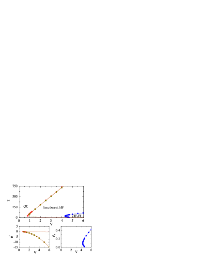
Figure 1: A phase diagram in the preformed heavy-fermion scenario, where QC, HF, and FL denote quantum critical, heavy fermion, and Fermi liquid, respectively. $T^{*}(V)$ corresponds to the mean-field transition temperature ($\rho_{b}=0$) in the Kondo breakdown theory while the Fermi-liquid temperature $T_{FL}(V)$ is much reduced due to quantum phase fluctuations of the hybridization order parameter ($\langle e^{i\theta_{b}}\rangle=0$). Reentrant behaviors are found in both $T^{*}$ and $T_{FL}$ numerically, but it is not clear whether this effect is fundamental or not due to quantum fluctuations. $\mu_{eff}^{\psi*}(V,T^{*})$ and $\rho_{b}(V,T_{FL})$ are also shown, where $m_{c}=0.01m_{f}$, $\mu=m_{f}^{-1}$, and $\epsilon_{f}=10m_{f}^{-1}$ are used with cutoffs of $\Lambda_{q}=\Lambda_{\nu}=10m_{f}^{-1}$ for the red-diamond and blue-circle lines and $\Lambda_{q}=\Lambda_{\nu}=50m_{f}^{-1}$ for the green-square line Supplementary . The unit of each axis is $m_{f}^{-1}$.

We perform the numerical analysis, where self-energy corrections are evaluated analytically. A detailed procedure can be found in our supplementary material Supplementary . Figure 1 displays the intermediate state, where $\rho_{b}$ is finite, resulting in the formation of the heavy-fermion band, while its coherence is not achieved yet, reflected in the fact that the chemical potential $-\mu_{eff}^{\psi}>0$. $T^{*}$ is characterized by $\rho_{b}(T^{*})=0$, and $T_{FL}$ is determined by $\mu_{eff}^{\psi}(T_{FL})=0$.

In the preformed heavy-fermion state the self-energy correction of $\psi$ is governed by Landau damping from incoherent heavy fermions, $\Delta\Sigma_{\psi}(q,i\Omega)=\gamma\frac{|\Omega|}{q}$, where the damping coefficient is given by $\gamma=V^{2}\rho_{b}\frac{\mathcal{K}_{F}^{f2}}{4\pi\mathcal{V}_{F}^{f}\mathcal{V}_{F}^{c}}$. Then, the imaginary part of the $\psi$ propagator becomes

$$-\Im G_{\psi}(q,\Omega)=\frac{\gamma\Omega q}{\gamma^{2}\Omega^{2}+q^{2}\Bigl{(}\frac{\rho_{b}}{2m_{b}}q^{2}-\mu_{eff}^{\psi}\Bigr{)}^{2}}.$$ (7)

This expression displays a crossover from $z=3$ to $z=1$ at $T_{1}\approx\frac{1}{\gamma}\sqrt{\frac{2m_{b}}{\rho_{b}}}(-\mu_{eff}^{\psi})^{\frac{3}{2}}$ as far as $T_{1}$ remains larger than $T_{FL}$. In $T_{FL}<T<T_{1}$, it is given by $-\Im G_{\psi}(q,\Omega)=\frac{\gamma\Omega q}{\gamma^{2}\Omega^{2}+\mu_{eff}^{\psi 2}q^{2}}$.

Inserting the $z=1$ propagator into self-energy equations for fermions, one finds that scattering with such fluctuations is less relevant for self-energy corrections of fermions than Fermi-liquid corrections in three dimensions. As a result, we expect that the $T$-linear resistivity due to scattering with $z=3$ critical modes KB_Indranil becomes smoothly transformed into the Fermi-liquid resistivity in the intermediate phase.

Recently, the $T^{*}$ line was proposed to be a Lifshitz transition Vojta_Lifshitz , motivated by the observation that isoelectronic chemical doping does not change $T^{*}$ while it affects the Néel temperature seriously brando . On the other hand, non-isoelectronic chemical doping changes $T^{*}$ clearly, when $Rh$ is replaced with $Fe$ Chemical_Doping_II . We believe that this issue should be clarified.

In conclusion, we uncovered a new incoherent heavy-fermion state which can be relevant to the nature of the intermediate region of $T_{FL}<T<T^{*}$. The mechanism turns out to be existence of quantum phase fluctuations in the hybridization order parameter. Despite the formation of the heavy-fermion band, this intermediate state will show non-Fermi liquid physics in transport and thermodynamics due to scattering with such $z=3$ soft modes. The non-Fermi liquid physics become transformed into the Fermi liquid physics continuously, as the $z=3$ critical mode turns into $z=1$, irrelevant for fermion dynamics.

This work was supported by the National Research Foundation of Korea (NRF) grant funded by the Korea government (MEST) (No. 2011-0074542). M.-T. was also supported by the Vietnamese NAFOSTED.

Appendix A To construct the Luttinger-Ward functional

Based on the nonlinear $\sigma$ model approach, we analyze an effective Lagrangian Eq. (3). Introducing $e^{i\theta_{b}}\rightarrow\psi$ with the unimodular constraint $|\psi|^{2}=1$, we rewrite Eq. (3) as follows

$${\cal L}\approx c_{\sigma}^{*}(\partial_{\tau}-\mu_{c})c_{\sigma}+\frac{1}{2m_{c}}|(\partial_{i}+iA_{i})c_{\sigma}|^{2}+\frac{V}{\sqrt{N}}\sqrt{\rho_{b}}(\psi^{*}c_{\sigma}^{*}f_{\sigma}+H.c.)$$

$$+f_{\sigma}^{*}(\partial_{\tau}-\mu_{c}+\epsilon_{f}+\lambda-ia_{\tau})f_{\sigma}+\frac{1}{2m_{f}}|(\partial_{i}-ia_{i})f_{\sigma}|^{2}$$

$$+\rho_{b}\psi^{*}(\partial_{\tau}+\lambda-ia_{\tau})\psi-\frac{1}{2u_{b}}[\psi^{*}(\partial_{\tau}+\lambda-ia_{\tau})\psi]^{2}+\frac{\rho_{b}}{2m_{b}}|(\partial_{i}-ia_{i}-iA_{i})\psi|^{2}-\mu_{\psi}(|\psi|^{2}-1)$$

$$+\frac{u_{b}}{2}\rho_{b}^{2}-\lambda SN+\frac{1}{4g^{2}}(\partial_{\mu}a_{\nu}-\partial_{\nu}a_{\mu})^{2},$$ (8)

where $\mu_{\psi}$ plays the role of an effective chemical potential, imposing the rotor constraint. As a result, three order parameters appear to be $\rho_{b}$, $\lambda$, and $\mu_{\psi}$ beyond the slave-boson mean-field analysis. Introduction of $\mu_{\psi}$ gives rise to a novel energy scale, determining the coherence of the heavy-fermion band.

One can derive an effective action from our effective field theory Eq. (A1), taking into account quantum corrections self-consistently in the Eliashberg approximation, where self-energy corrections are introduced, but vertex corrections are neglected. The Eliashberg approximation results in the following effective action

$$S=\int_{0}^{\beta}d\tau\int d^{3}r\int_{0}^{\beta}d\tau^{\prime}\int d^{3}r^{\prime}\Bigl{[}c_{\sigma}^{*}(r,\tau)\Bigl{\{}\Bigl{(}\partial_{\tau}-\mu_{c}-\frac{\partial_{i}^{2}}{2m_{c}}\Bigr{)}\delta(\tau-\tau^{\prime})\delta^{3}(r-r^{\prime})+\Sigma_{c}(r-r^{\prime},\tau-\tau^{\prime})\Bigr{\}}c_{\sigma}(r^{\prime},\tau^{\prime})$$

$$-N\Sigma_{c}(r-r^{\prime},\tau-\tau^{\prime})G_{c}(r^{\prime}-r,\tau^{\prime}-\tau)\Bigr{]}$$

$$+\int_{0}^{\beta}d\tau\int d^{3}r\int_{0}^{\beta}d\tau^{\prime}\int d^{3}r^{\prime}\Bigl{[}f_{\sigma}^{*}(r,\tau)\Bigl{\{}\Bigl{(}\partial_{\tau}-\mu_{c}+\epsilon_{f}+\lambda-\frac{\partial_{i}^{2}}{2m_{f}}\Bigr{)}\delta(\tau-\tau^{\prime})\delta^{3}(r-r^{\prime})+\Sigma_{f}(r-r^{\prime},\tau-\tau^{\prime})\Bigr{\}}f_{\sigma}(r^{\prime},\tau^{\prime})$$

$$-N\Sigma_{f}(r-r^{\prime},\tau-\tau^{\prime})G_{f}(r^{\prime}-r,\tau^{\prime}-\tau)\Bigr{]}$$

$$+\int_{0}^{\beta}d\tau\int d^{3}r\int_{0}^{\beta}d\tau^{\prime}\int d^{3}r^{\prime}\Bigl{[}\psi^{*}(r,\tau)\Bigl{\{}\Bigl{(}[\rho_{b}-\lambda/u_{b}]\partial_{\tau}-\frac{1}{2u_{b}}\partial_{\tau}^{2}-\mu_{\psi}+\rho_{b}\lambda-\frac{\rho_{b}}{2m_{b}}\partial_{i}^{2}\Bigr{)}\delta(\tau-\tau^{\prime})\delta^{3}(r-r^{\prime})$$

$$+\Sigma_{\psi}(r-r^{\prime},\tau-\tau^{\prime})\Bigr{\}}\psi(r^{\prime},\tau^{\prime})+\Sigma_{\psi}(r-r^{\prime},\tau-\tau^{\prime})G_{\psi}(r^{\prime}-r,\tau^{\prime}-\tau)\Bigr{]}$$

$$+\int_{0}^{\beta}d\tau\int d^{3}r\int_{0}^{\beta}d\tau^{\prime}\int d^{3}r^{\prime}\Bigl{[}\frac{1}{2}a_{\mu}(r,\tau)\Bigl{\{}\Bigl{(}-\frac{\partial_{\tau}^{2}+\partial_{i}^{2}}{g^{2}}\Bigr{)}P_{\mu\nu}^{T}\delta(\tau-\tau^{\prime})\delta^{3}(r-r^{\prime})+\Pi_{\mu\nu}(r-r^{\prime},\tau-\tau^{\prime})\Bigr{\}}a_{\nu}(r^{\prime},\tau^{\prime})$$

$$+\Pi_{\mu\nu}(r-r^{\prime},\tau-\tau^{\prime})D_{\mu\nu}(r^{\prime}-r,\tau^{\prime}-\tau)\Bigr{]}$$

$$-V^{2}\rho_{b}\int_{0}^{\beta}d\tau\int d^{3}r\int_{0}^{\beta}d\tau^{\prime}\int d^{3}r^{\prime}G_{\psi}(r-r^{\prime},\tau-\tau^{\prime})G_{f}(r^{\prime}-r,\tau^{\prime}-\tau)G_{c}(r-r^{\prime},\tau-\tau^{\prime})$$

$$-\frac{N}{2}\int_{0}^{\beta}d\tau\int d^{3}r\int_{0}^{\beta}d\tau^{\prime}\int d^{3}r^{\prime}v_{\mu}^{f}D_{\mu\nu}(r-r^{\prime},\tau-\tau^{\prime})v_{\nu}^{f}G_{f}(r^{\prime}-r,\tau^{\prime}-\tau)G_{f}(r-r^{\prime},\tau-\tau^{\prime})$$

$$-\frac{1}{2}\int_{0}^{\beta}d\tau\int d^{3}r\int_{0}^{\beta}d\tau^{\prime}\int d^{3}r^{\prime}v_{\mu}^{\psi}D_{\mu\nu}(r-r^{\prime},\tau-\tau^{\prime})v_{\nu}^{\psi}G_{\psi}(r^{\prime}-r,\tau^{\prime}-\tau)G_{\psi}(r-r^{\prime},\tau-\tau^{\prime})$$

$$-\beta L^{3}\Bigl{(}\frac{\lambda^{2}}{2u_{b}}-\mu_{\psi}-\frac{u_{b}}{2}\rho_{b}^{2}+NS\lambda\Bigr{)},$$ (9)

where $\Sigma_{c}(r-r^{\prime},\tau-\tau^{\prime})$, $\Sigma_{f}(r-r^{\prime},\tau-\tau^{\prime})$, $\Sigma_{\psi}(r-r^{\prime},\tau-\tau^{\prime})$, and $\Pi_{\mu\nu}(r-r^{\prime},\tau-\tau^{\prime})$ are self-energy corrections of electrons, spinons, $\psi$, and gauge fields, respectively, and $G_{c}(r-r^{\prime},\tau-\tau^{\prime})$, $G_{f}(r-r^{\prime},\tau-\tau^{\prime})$, $G_{\psi}(r-r^{\prime},\tau-\tau^{\prime})$, and $D_{\mu\nu}(r-r^{\prime},\tau-\tau^{\prime})$ are their Green’s functions. Although vertex corrections are neglected for self-energy calculations, such contributions are introduced self-consistently into three coupled equations for order parameters. A way how to derive this effective action is shown in Ref. Kim_LW .

Performing the Fourier transformation and integrating over all field variables, we find the Luttinger-Ward functional

$$F_{LW}[\Sigma_{c}(k,i\omega),\Sigma_{f}(k,i\omega),\Sigma_{\psi}(q,i\Omega),\Pi_{ij}(q,i\Omega),\rho_{b},\lambda,\mu_{\psi}]=-L^{3}\Bigl{(}\frac{\lambda^{2}}{2u_{b}}-\mu_{\psi}-\frac{u_{b}}{2}\rho_{b}^{2}+NS\lambda\Bigr{)}$$

$$-\frac{N}{\beta}\sum_{i\omega}\int\frac{d^{3}k}{(2\pi)^{3}}\Bigl{\{}\ln\Bigl{(}-G_{c}^{-1}(k,i\omega)\Bigr{)}+\Sigma_{c}(k,i\omega)G_{c}(k,i\omega)\Bigr{\}}$$

$$-\frac{N}{\beta}\sum_{i\omega}\int\frac{d^{3}k}{(2\pi)^{3}}\Bigl{\{}\ln\Bigl{(}-G_{f}^{-1}(k,i\omega)\Bigr{)}+\Sigma_{f}(k,i\omega)G_{f}(k,i\omega)\Bigr{\}}$$

$$+\frac{1}{\beta}\sum_{i\Omega}\int\frac{d^{3}q}{(2\pi)^{3}}\Bigl{\{}\ln\Bigl{(}-G_{\psi}^{-1}(q,i\Omega)\Bigr{)}+\Sigma_{\psi}(q,i\Omega)G_{\psi}(q,i\Omega)\Bigr{\}}$$

$$+\frac{1}{\beta}\sum_{i\Omega}\int\frac{d^{3}q}{(2\pi)^{3}}\Bigl{\{}\ln\Bigl{(}-D^{-1}(q,i\Omega)\Bigr{)}+\Pi(q,i\Omega)D(q,i\Omega)\Bigr{\}}$$

$$-V^{2}\rho_{b}\frac{1}{\beta}\sum_{i\omega}\int\frac{d^{3}k}{(2\pi)^{3}}\frac{1}{\beta}\sum_{i\Omega}\int\frac{d^{3}q}{(2\pi)^{3}}G_{\psi}(q,i\Omega)G_{f}(k,i\omega)G_{c}(k+q,i\omega+i\Omega)$$

$$-\frac{N}{2}\frac{1}{\beta}\sum_{i\omega}\int\frac{d^{3}k}{(2\pi)^{3}}\frac{1}{\beta}\sum_{i\Omega}\int\frac{d^{3}q}{(2\pi)^{3}}F(k,q)D(q,i\Omega)G_{f}(k,i\omega)G_{f}(k+q,i\omega+i\Omega)$$

$$-\frac{\rho_{b}^{2}}{2}\frac{1}{\beta}\sum_{i\Omega}\int\frac{d^{3}q}{(2\pi)^{3}}\frac{1}{\beta}\sum_{i\nu}\int\frac{d^{3}l}{(2\pi)^{3}}B(q,l)D(l,i\nu)G_{\psi}(q,i\Omega)G_{\psi}(q+l,i\Omega+i\nu),$$ (10)

where $G_{c}(k,i\omega)$, $G_{f}(k,i\omega)$, $G_{\psi}(k,i\omega)$, and $D(q,i\Omega)$ are Green’s functions of electrons, spinons, phases, and gauge fields, respectively, given by

$$G_{c}(k,i\omega)=\frac{1}{i\omega+\mu_{c}-\frac{k^{2}}{2m_{c}}-\Sigma_{c}(k,i\omega)},~{}~{}~{}~{}~{}G_{f}(k,i\omega)=\frac{1}{i\omega+\mu_{c}-\epsilon_{f}-\lambda-\frac{k^{2}}{2m_{f}}-\Sigma_{f}(k,i\omega)},$$

$$G_{\psi}(q,i\Omega)=\frac{1}{(\rho_{b}-\lambda/u_{b})(i\Omega)-\frac{\Omega^{2}}{2u_{b}}-\frac{\rho_{b}}{2m_{b}}q^{2}+\mu_{\psi}-\rho_{b}\lambda-\Sigma_{\psi}(q,i\Omega)},$$

$$D(q,i\Omega)=-\frac{1}{\frac{\Omega^{2}+q^{2}}{g^{2}}+\Pi(q,i\Omega)},~{}~{}~{}~{}~{}D_{ij}(q,i\Omega)=D(q,i\Omega)P_{ij}^{T}(q),~{}~{}~{}~{}~{}\Pi_{ij}(q,i\Omega)=\Pi(q,i\Omega)P_{ij}^{T}(q).$$ (11)

$P_{ij}^{T}(q)$ is the projection operator to the transverse component, and

$$F(k,q)=\frac{1}{2}\sum_{i,j=1}^{2}v_{i}^{f}\Bigl{(}\delta_{ij}-\frac{q_{i}q_{j}}{q^{2}}\Bigr{)}v_{j}^{f},~{}~{}~{}~{}~{}v_{i}^{f}=\frac{k_{i}+q_{i}/2}{m_{f}},$$

$$B(q,l)=\frac{1}{2}\sum_{i,j=1}^{2}v_{i}^{\psi}\Bigl{(}\delta_{ij}-\frac{l_{i}l_{j}}{l^{2}}\Bigr{)}v_{j}^{\psi},~{}~{}~{}~{}~{}v_{i}^{\psi}=\frac{q_{i}+l_{i}/2}{m_{b}},$$

where $v_{i}^{f}$ and $v_{i}^{\psi}$ are velocities of spinons and phases in the $i$-direction.

Minimizing the free energy functional with respect to all self-energies, we obtain self-consistent Eliashberg equations

$$\Sigma_{c}(k,i\omega)=-\frac{V^{2}\rho_{b}}{N}\frac{1}{\beta}\sum_{i\Omega}\int\frac{d^{3}q}{(2\pi)^{3}}G_{\psi}(q,i\Omega)G_{f}(k-q,i\omega-i\Omega),$$

$$\Sigma_{f}(k,i\omega)=-\frac{V^{2}\rho_{b}}{N}\frac{1}{\beta}\sum_{i\Omega}\int\frac{d^{3}q}{(2\pi)^{3}}G_{\psi}(q,i\Omega)G_{c}(k+q,i\omega+i\Omega)-\frac{1}{\beta}\sum_{i\Omega}\int\frac{d^{3}q}{(2\pi)^{3}}F(k,q)D(q,i\Omega)G_{f}(k,i\omega),$$

$$\Sigma_{\psi}(q,i\Omega)=V^{2}\rho_{b}\frac{1}{\beta}\sum_{i\omega}\int\frac{d^{3}k}{(2\pi)^{3}}G_{f}(k,i\omega)G_{c}(k+q,i\omega+i\Omega)+\rho_{b}^{2}\frac{1}{\beta}\sum_{i\nu}\int\frac{d^{3}l}{(2\pi)^{3}}B(q,l)D(l,i\nu)G_{\psi}(q+l,i\Omega+i\nu),$$

$$\Pi(q,i\Omega)=\frac{N}{2}\frac{1}{\beta}\sum_{i\omega}\int\frac{d^{3}k}{(2\pi)^{3}}F(k,q)G_{f}(k,i\omega)G_{f}(k+q,i\omega+i\Omega)+\frac{\rho_{b}^{2}}{2}\frac{1}{\beta}\sum_{i\nu}\int\frac{d^{3}l}{(2\pi)^{3}}B(q,l)G_{\psi}(q,i\Omega)G_{\psi}(q+l,i\Omega+i\nu).$$

We note that these equations are essentially the same as those in the quantum critical regime of the Kondo breakdown theory KB_Indranil ; KB_Pepin , where the self-energy and Green’s function of $\psi$ are identified with those of $b$.

Appendix B To evaluate self-energy corrections

B.1 Self-energy corrections for the heavy-fermion band

In order to describe the heavy-fermion band without condensation of $\psi$, we separate fermion self-energy corrections as follows

$$\Sigma_{c}(k,i\omega)=\Phi_{c}(k,i\omega)+\Delta\Sigma_{c}(i\omega),~{}~{}~{}~{}~{}\Sigma_{f}(k,i\omega)=\Phi_{f}(k,i\omega)+\Delta\Sigma_{f}(i\omega),$$ (13)

where $\Phi_{c}(k,i\omega)$ and $\Phi_{f}(k,i\omega)$ are associated with the formation of the heavy-fermion band, and $\Delta\Sigma_{c}(i\omega)$ and $\Delta\Sigma_{f}(i\omega)$ are related with non-Fermi liquid physics of such heavy fermions.

Static contributions of bosons determine the formation of the heavy-fermion band, given by

$$\Phi_{c}(k,i\omega)=-\frac{TV^{2}\rho_{b}}{N}G_{\psi}(0,0)G_{f}(k,i\omega)=-\frac{V^{2}\rho_{b}}{N}\frac{T}{|\mu_{eff}^{\psi}|}G_{f}(k,i\omega)\approx-\frac{V^{2}\rho_{b}}{N}\frac{T}{|\mu_{eff}^{\psi}|}g_{f}(k,i\omega),$$

$$\Phi_{f}(k,i\omega)=-\frac{TV^{2}\rho_{b}}{N}G_{\psi}(0,0)G_{c}(k,i\omega)=-\frac{V^{2}\rho_{b}}{N}\frac{T}{|\mu_{eff}^{\psi}|}G_{c}(k,i\omega)\approx-\frac{V^{2}\rho_{b}}{N}\frac{T}{|\mu_{eff}^{\psi}|}g_{c}(k,i\omega),$$ (14)

where

$$\mu_{eff}^{\psi}=\mu_{\psi}-\rho_{b}\lambda-\Sigma_{\psi}(0,0)$$ (15)

is an effective chemical potential, essential for coherence. When it touches zero, $\frac{T}{|\mu_{eff}^{\psi}|}$ should be replaced with $|\langle\psi\rangle|^{2}$.

$$g_{c}(k,i\omega)=\frac{1}{i\omega+\mu_{c}-\frac{k^{2}}{2m_{c}}},~{}~{}~{}~{}~{}g_{f}(k,i\omega)=\frac{1}{i\omega+\mu_{c}-\epsilon_{f}-\lambda-\frac{k^{2}}{2m_{f}}}$$ (16)

are bare Green’s functions.

Quantum fluctuations of bosons give rise to non-Fermi liquid self-energy corrections of such heavy fermions

$$\Delta\Sigma_{c}(i\omega)=-\frac{V^{2}\rho_{b}}{N}\frac{1}{\beta}\sum_{i\Omega\not=0}\int_{q\not=0}\frac{d^{3}q}{(2\pi)^{3}}G_{\psi}(q,i\Omega)G_{f}(k-q,i\omega-i\Omega),$$

$$\Delta\Sigma_{f}(i\omega)=-\frac{V^{2}\rho_{b}}{N}\frac{1}{\beta}\sum_{i\Omega\not=0}\int_{q\not=0}\frac{d^{3}q}{(2\pi)^{3}}G_{\psi}(q,i\Omega)G_{c}(k+q,i\omega+i\Omega)-\frac{1}{\beta}\sum_{i\Omega\not=0}\int_{q\not=0}\frac{d^{3}q}{(2\pi)^{3}}F(k,q)D(q,i\Omega)G_{f}(k,i\omega),$$

where the static component of the $\psi$ propagator should not be taken into account.

For convenience, we also divide the $\psi$ self-energy as follows

$$\Sigma_{\psi}(q,i\Omega)=\Sigma_{\psi}(0,0)+\Delta\Sigma_{\psi}(q,i\Omega),$$ (18)

where the static contribution is introduced into the effective chemical potential, given by

$$\Sigma_{\psi}(0,0)=V^{2}\rho_{b}\frac{1}{\beta}\sum_{i\omega}\int\frac{d^{3}k}{(2\pi)^{3}}G_{f}(k,i\omega)G_{c}(k,i\omega)\approx-\frac{V^{2}\rho_{b}}{2\pi^{2}}\frac{\mathcal{K}_{F}^{c2}}{\mathcal{V}_{F}^{c}},$$ (19)

and the dynamic part results in Landau damping, given by

$$\Delta\Sigma_{\psi}(q,i\Omega)=V^{2}\rho_{b}\frac{1}{\beta}\sum_{i\omega}\int\frac{d^{3}k}{(2\pi)^{3}}G_{f}(k,i\omega)G_{c}(k+q,i\omega+i\Omega)+\rho_{b}^{2}\frac{1}{\beta}\sum_{i\nu}\int\frac{d^{3}l}{(2\pi)^{3}}B(q,l)D(l,i\nu)G_{\psi}(q+l,i\Omega+i\nu).$$

In the next subsection we evaluate this dynamic contribution, where the self-energy correction from gauge fluctuations (the second term) will not be taken into account. That contribution is irrelevant because the $\psi$ dynamics is described by $z=3$, which implies that the effective theory for the $\psi$ dynamics lies above the upper critical dimension, resulting in the mean-field-like dynamics. See our discussion on this issue in the last section.

B.2 To calculate the $\psi$ self-energy

In order to cover both the quantum critical regime and the incoherent heavy-fermion phase, we introduce the following fermion Green’s functions

$$G_{f}(i\omega,k)=\frac{1}{i\omega-v_{F}^{f}(k-k_{F}^{f})-\frac{TV^{2}\rho_{b}/|\mu_{eff}^{\psi}|}{i\omega-v_{F}^{c}(k-k_{F}^{c})}-\Delta\Sigma_{f}(i\omega)},$$

$$G_{c}(i\omega,k)=\frac{1}{i\omega-v_{F}^{c}(k-k_{F}^{c})-\frac{TV^{2}\rho_{b}/|\mu_{eff}^{\psi}|}{i\omega-v_{F}^{f}(k-k_{F}^{f})}-\Delta\Sigma_{c}(i\omega)}.$$ (21)

$\Delta\Sigma_{f(c)}(i\omega)$ is the spinon (electron) self-energy due to inelastic scattering with quantum phase fluctuations, where the heavy-fermion contribution of $\Phi_{f(c)}(k,i\omega)$ is expressed explicitly. We emphasize that there is $T/|\mu_{eff}^{\psi}|$, renormalizing $\rho_{b}$, which reduces the strength of hybridization due to incoherence. We have linearized each bare dispersion, where $v_{F}^{f(c)}$ is the Fermi velocity and $k_{F}^{f(c)}$ is the Fermi momentum.

Neglecting non-Fermi liquid parts of self-energy corrections for the time being, we can express Eq. (B9) as follows

$$G_{f/c}(\omega,k)=\frac{Z_{f/c}}{\omega-\mathcal{V}^{f/c}_{F}(k-\mathcal{K}_{F}^{f/c})},$$ (22)

where $\mathcal{V}^{f/c}_{F}$ and $\mathcal{K}_{F}^{f/c}$ are renormalized Fermi velocity and renormalized Fermi momentum, respectively, and $Z_{f/c}$ is the wave-function renormalization function. They are given by

$$\mathcal{K}_{F}^{f}=\mathcal{K}_{F}^{c}=\frac{1}{2}\left(k_{F}^{f}+k_{F}^{c}\right)+\frac{1}{2}\sqrt{\left(k_{F}^{f}-k_{F}^{c}\right)^{2}+4\frac{TV^{2}\rho_{b}/|\mu_{eff}^{\psi}|}{v_{F}^{f}v_{F}^{c}}},$$

$$\mathcal{V}_{F}^{f/c}=Z_{f/c}\left[v_{F}^{f/c}+\frac{(TV^{2}\rho_{b}/|\mu_{eff}^{\psi}|)v_{F}^{c/f}}{\left(v_{F}^{c/f}\right)^{2}\left(\mathcal{K}_{F}-k_{F}^{c/f}\right)^{2}}\right],~{}~{}~{}Z_{f/c}^{-1}=1+\frac{TV^{2}\rho_{b}/|\mu_{eff}^{\psi}|}{\left(v_{F}^{c/f}\right)^{2}\left(\mathcal{K}_{F}-k_{F}^{c/f}\right)^{2}}.$$ (23)

Inserting Eq. (B9) with Eq. (B10) into the $\psi$ self-energy, we obtain the following expression KB_Indranil ; KB_Pepin

$$\Delta\Sigma_{\psi}(i\Omega,\mathbf{q})=V^{2}\rho_{b}\frac{1}{\beta}\sum\limits_{i\omega}\int\frac{d^{3}k}{(2\pi)^{3}}G_{f}(i\omega,\mathbf{k})G_{c}(i\omega+i\Omega,\mathbf{k+q})$$

$$=V^{2}\rho_{b}\frac{(\mathcal{K}_{F}^{f})^{2}}{4\pi^{2}\mathcal{V}_{F}^{f}\mathcal{V}_{F}^{c}}\frac{1}{\alpha-1}\frac{1}{q}\Bigl{\{}\Bigl{(}\alpha i\Omega+\mathcal{V}_{F}^{f}(\mathcal{K}_{F}^{c}-\mathcal{K}_{F}^{f})\Bigr{)}\log\Bigl{(}\frac{\alpha i\Omega+\mathcal{V}_{F}^{f}(\mathcal{K}_{F}^{c}-\mathcal{K}_{F}^{f})+\alpha\mathcal{V}_{F}^{c}q}{\alpha i\Omega+\mathcal{V}_{F}^{f}(\mathcal{K}_{F}^{c}-\mathcal{K}_{F}^{f})-\alpha\mathcal{V}_{F}^{c}q}\Bigr{)}$$

$$-\Bigl{(}i\Omega+\mathcal{V}_{F}^{f}(\mathcal{K}_{F}^{c}-\mathcal{K}_{F}^{f})\Bigr{)}\log\Bigl{(}\frac{i\Omega+\mathcal{V}_{F}^{f}(\mathcal{K}_{F}^{c}-\mathcal{K}_{F}^{f})+\alpha\mathcal{V}_{F}^{c}q}{i\Omega+\mathcal{V}_{F}^{f}(\mathcal{K}_{F}^{c}-\mathcal{K}_{F}^{f})-\alpha\mathcal{V}_{F}^{c}q}\Bigr{)}$$

$$+\alpha\mathcal{V}_{F}^{c}q\log\Bigl{(}\frac{(\alpha i\Omega+\mathcal{V}_{F}^{f}(\mathcal{K}_{F}^{c}-\mathcal{K}_{F}^{f}))^{2}-(\alpha\mathcal{V}_{F}^{c}q)^{2}}{(i\Omega+\mathcal{V}_{F}^{f}(\mathcal{K}_{F}^{c}-\mathcal{K}_{F}^{f}))^{2}-(\alpha\mathcal{V}_{F}^{c}q)^{2}}\Bigr{)}\Bigr{\}}$$ (24)

with $\alpha=\frac{\mathcal{V}_{F}^{f}}{\mathcal{V}_{F}^{c}}$. Taking $\alpha\rightarrow 1$ with $\mathcal{K}_{F}^{c}=\mathcal{K}_{F}^{f}$ for the heavy-fermion band, this expression is simplified as

$$\Delta\Sigma_{\psi}(i\Omega,\mathbf{q})=V^{2}\rho_{b}\frac{(\mathcal{K}_{F}^{f})^{2}}{4\pi^{2}\mathcal{V}_{F}^{f}\mathcal{V}_{F}^{c}}\frac{1}{q}\Bigl{\{}i\Omega\ln\frac{i\Omega+\mathcal{V}_{F}^{c}q}{i\Omega-\mathcal{V}_{F}^{c}q}+i\Omega\Bigl{(}\frac{\mathcal{V}_{F}^{c}q}{i\Omega+\mathcal{V}_{F}^{c}q}+\frac{\mathcal{V}_{F}^{c}q}{i\Omega-\mathcal{V}_{F}^{c}q}\Bigr{)}+2\mathcal{V}_{F}^{c}q\frac{(i\Omega)^{2}}{(i\Omega)^{2}-(\mathcal{V}_{F}^{c}q)^{2}}\Bigr{\}}.$$ (25)

If one expands Eq. (B12) in the limit of $\frac{\mathcal{K}^{f}_{F}-\mathcal{K}^{c}_{F}}{q}\ll 1$, the typical Landau damping form results

$$\Sigma_{\psi}(i\Omega,q)=\gamma\frac{|\Omega|}{q},$$ (26)

originating from particle-hole excitations around the Fermi surface. The damping coefficient is given by

$$\gamma=V^{2}\rho_{b}\frac{(\mathcal{K}_{F}^{f})^{2}}{4\pi\mathcal{V}_{F}^{f}\mathcal{V}_{F}^{c}}.$$ (27)

Then, the $\psi$ propagator becomes

$$G_{\psi}(q,i\Omega)\approx-\frac{1}{\gamma\frac{|\Omega|}{q}+\frac{\rho_{b}}{2m_{b}}q^{2}-\mu_{eff}^{\psi}},$$ (28)

where $\mu_{eff}^{\psi}=\mu_{\psi}-\rho_{b}\lambda-\Sigma_{\psi}(0,0)$ is an effective chemical potential for phase fluctuations.

Inserting this boson propagator into self-energy equations for fermions, one can find fermion self-energy corrections. Such calculations have been performed in previous studies KB_Indranil ; KB_Pepin when the boson dynamics is critical and described by $z=3$. Since the $\psi$ dynamics is also characterized by $z=3$ when $T>T_{1}$, as discussed in the manuscript, the previous results are applied to the present situation directly. Then, we obtain non-Fermi liquid self-energies.

Appendix C To derive self-consistent equations for three order parameters of $\rho_{b}$, $\lambda$, and $\mu_{\psi}$

C.1 General formulae

One can find self-consistent equations for order parameters from the Luttinger-Ward free energy functional. An essential merit of this approach is that vertex corrections are naturally introduced beyond the Schwinger-Dyson equation for an order parameter usually identified with the mean-field equation.

Minimizing the free energy functional with respect to $\rho_{b}$, we obtain

$$u_{b}\rho_{b}+\frac{N}{\beta}\sum_{i\omega}\int\frac{d^{3}k}{(2\pi)^{3}}\frac{\partial\Sigma_{c}(k,i\omega)}{\partial\rho_{b}}G_{c}(k,i\omega)+\frac{N}{\beta}\sum_{i\omega}\int\frac{d^{3}k}{(2\pi)^{3}}\frac{\partial\Sigma_{f}(k,i\omega)}{\partial\rho_{b}}G_{f}(k,i\omega)$$

$$+\frac{1}{\beta}\sum_{i\Omega}\int\frac{d^{3}q}{(2\pi)^{3}}\Bigl{(}i\Omega-\frac{q^{2}}{2m_{b}}-\lambda-\frac{\partial\Sigma_{\psi}(k,i\omega)}{\partial\rho_{b}}\Bigr{)}G_{\psi}(q,i\Omega)+\frac{1}{\beta}\sum_{i\Omega}\int\frac{d^{3}q}{(2\pi)^{3}}\frac{\partial\Pi(q,i\Omega)}{\partial\rho_{b}}D(q,i\Omega)=0,$$ (29)

where the derivative for each self-energy implies each vertex correction. In particular, we see that $\frac{\partial\Sigma_{\psi}(k,i\omega)}{\partial\rho_{b}}$ is the vertex correction, performed in the single impurity problem Read_KI . Such a contribution is expected to modify the slave-boson mean-field equation for $\rho_{b}$ in principle.

Minimizing the free energy functional with respect to $\lambda$, we obtain

$$-\frac{\lambda}{u_{b}}-NS+\frac{N}{\beta}\sum_{i\omega}\int\frac{d^{3}k}{(2\pi)^{3}}\frac{\partial\Sigma_{c}(k,i\omega)}{\partial\lambda}G_{c}(k,i\omega)+\frac{N}{\beta}\sum_{i\omega}\int\frac{d^{3}k}{(2\pi)^{3}}\Bigl{(}1+\frac{\partial\Sigma_{f}(k,i\omega)}{\partial\lambda}\Bigr{)}G_{f}(k,i\omega)$$

$$+\frac{1}{\beta}\sum_{i\Omega}\int\frac{d^{3}q}{(2\pi)^{3}}\Bigl{(}-\frac{1}{u_{b}}i\Omega-\rho_{b}-\frac{\partial\Sigma_{\psi}(k,i\omega)}{\partial\lambda}\Bigr{)}G_{\psi}(q,i\Omega)+\frac{1}{\beta}\sum_{i\Omega}\int\frac{d^{3}q}{(2\pi)^{3}}\frac{\partial\Pi(q,i\Omega)}{\partial\lambda}D(q,i\Omega)=0,$$ (30)

where $\frac{\partial\Sigma_{\psi}(k,i\omega)}{\partial\lambda}$ is the vertex correction beyond the slave-boson mean-field analysis.

In the same way we find an equation for $\mu_{\psi}$, given by

$$1+\frac{N}{\beta}\sum_{i\omega}\int\frac{d^{3}k}{(2\pi)^{3}}\frac{\partial\Sigma_{c}(k,i\omega)}{\partial\mu_{\psi}}G_{c}(k,i\omega)+\frac{N}{\beta}\sum_{i\omega}\int\frac{d^{3}k}{(2\pi)^{3}}\frac{\partial\Sigma_{f}(k,i\omega)}{\partial\mu_{\psi}}G_{f}(k,i\omega)$$

$$+\frac{1}{\beta}\sum_{i\Omega}\int\frac{d^{3}q}{(2\pi)^{3}}\Bigl{(}1-\frac{\partial\Sigma_{\psi}(k,i\omega)}{\partial\mu_{\psi}}\Bigr{)}G_{\psi}(q,i\Omega)+\frac{1}{\beta}\sum_{i\Omega}\int\frac{d^{3}q}{(2\pi)^{3}}\frac{\partial\Pi(q,i\Omega)}{\partial\mu_{\psi}}D(q,i\Omega)=0,$$ (31)

where $\frac{\partial\Sigma_{c}(k,i\omega)}{\partial\mu_{\psi}}$ and $\frac{\partial\Sigma_{f}(k,i\omega)}{\partial\mu_{\psi}}$ are identified with vertex corrections.

C.2 An equation for $\mu_{\psi}$

We analyze the equation for $\mu_{\psi}$. Inserting both fermion self-energies associated with the heavy-fermion band and boson self-energy into Eq. (C3), we obtain

$$1-\frac{N}{\beta}\sum_{i\omega}\int\frac{d^{3}k}{(2\pi)^{3}}\Bigl{\{}\frac{\partial}{\partial\mu_{\psi}}\Bigl{(}\frac{V^{2}\rho_{b}}{N}\frac{T}{|\mu_{eff}^{\psi}|}g_{f}(k,i\omega)\Bigr{)}\Bigr{\}}G_{c}(k,i\omega)-\frac{N}{\beta}\sum_{i\omega}\int\frac{d^{3}k}{(2\pi)^{3}}\Bigl{\{}\frac{\partial}{\partial\mu_{\psi}}\Bigl{(}\frac{V^{2}\rho_{b}}{N}\frac{T}{|\mu_{eff}^{\psi}|}g_{c}(k,i\omega)\Bigr{)}\Bigr{\}}G_{f}(k,i\omega)$$

$$+\frac{1}{\beta}\sum_{i\Omega}\int\frac{d^{3}q}{(2\pi)^{3}}\Bigl{\{}1+\frac{\partial}{\partial\mu_{\psi}}\Bigl{(}\frac{V^{2}\rho_{b}}{2\pi^{2}}\frac{\mathcal{K}_{F}^{c2}}{\mathcal{V}_{F}^{c}}\Bigr{)}-\frac{\partial}{\partial\mu_{\psi}}\Bigl{(}\gamma\frac{|\Omega|}{q}\Bigr{)}\Bigr{\}}G_{\psi}(q,i\Omega)=0.$$ (32)

We rearrange this equation as follows

$$1+\frac{1}{\beta}\sum_{i\Omega}\int\frac{d^{3}q}{(2\pi)^{3}}G_{\psi}(q,i\Omega)+\frac{1}{\beta}\sum_{i\Omega}\int\frac{d^{3}q}{(2\pi)^{3}}\Bigl{\{}\frac{\partial}{\partial\mu_{\psi}}\Bigl{(}\frac{V^{2}\rho_{b}}{2\pi^{2}}\frac{\mathcal{K}_{F}^{c2}}{\mathcal{V}_{F}^{c}}\Bigr{)}-\frac{\partial}{\partial\mu_{\psi}}\Bigl{(}\gamma\frac{|\Omega|}{q}\Bigr{)}\Bigr{\}}G_{\psi}(q,i\Omega)$$

$$=\frac{N}{\beta}\sum_{i\omega}\int\frac{d^{3}k}{(2\pi)^{3}}\Bigl{\{}\frac{\partial}{\partial\mu_{\psi}}\Bigl{(}\frac{V^{2}\rho_{b}}{N}\frac{T}{|\mu_{eff}^{\psi}|}g_{f}(k,i\omega)\Bigr{)}\Bigr{\}}G_{c}(k,i\omega)+\frac{N}{\beta}\sum_{i\omega}\int\frac{d^{3}k}{(2\pi)^{3}}\Bigl{\{}\frac{\partial}{\partial\mu_{\psi}}\Bigl{(}\frac{V^{2}\rho_{b}}{N}\frac{T}{|\mu_{eff}^{\psi}|}g_{c}(k,i\omega)\Bigr{)}\Bigr{\}}G_{f}(k,i\omega).$$

This expression is quite interesting in the respect that the first two terms in the left-hand-side correspond to the Schwinger-Dyson equation resulting from $\langle|\psi|^{2}\rangle$ = 1 while other contributions originate from vertex corrections.

Keeping $\mu_{\psi}$-derivative terms only when they depend on $\mu_{\psi}$ explicitly as the lowest-order approximation, we reach the following expression

$$1-\frac{TV^{2}\rho_{b}}{\mu_{eff}^{\psi 2}}\Bigl{\{}\frac{1}{\beta}\sum_{i\omega}\int\frac{d^{3}k}{(2\pi)^{3}}g_{f}(k,i\omega)G_{c}(k,i\omega)+\frac{1}{\beta}\sum_{i\omega}\int\frac{d^{3}k}{(2\pi)^{3}}g_{c}(k,i\omega)G_{f}(k,i\omega)\Bigr{\}}=-\frac{1}{\beta}\sum_{i\Omega}\int\frac{d^{3}q}{(2\pi)^{3}}G_{\psi}(q,i\Omega).$$

It is clear that fermion contributions are related with vertex corrections. We will see that this correction plays an important role for self-consistency, which cancels other quantum corrections.

C.3 An equation for $\rho_{b}$

Inserting both fermion self-energies associated with the heavy-fermion band and boson self-energy into Eq. (C1), we obtain

$$u_{b}\rho_{b}-\frac{N}{\beta}\sum_{i\omega}\int\frac{d^{3}k}{(2\pi)^{3}}\Bigl{\{}\frac{\partial}{\partial\rho_{b}}\Bigl{(}\frac{V^{2}\rho_{b}}{N}\frac{T}{|\mu_{eff}^{\psi}|}g_{f}(k,i\omega)\Bigr{)}\Bigr{\}}G_{c}(k,i\omega)-\frac{N}{\beta}\sum_{i\omega}\int\frac{d^{3}k}{(2\pi)^{3}}\Bigl{\{}\frac{\partial}{\partial\rho_{b}}\Bigl{(}\frac{V^{2}\rho_{b}}{N}\frac{T}{|\mu_{eff}^{\psi}|}g_{c}(k,i\omega)\Bigr{)}\Bigr{\}}G_{f}(k,i\omega)$$

$$+\frac{1}{\beta}\sum_{i\Omega}\int\frac{d^{3}q}{(2\pi)^{3}}\Bigl{\{}i\Omega-\frac{q^{2}}{2m_{b}}-\lambda+\frac{\partial}{\partial\rho_{b}}\Bigl{(}\frac{V^{2}\rho_{b}}{2\pi^{2}}\frac{\mathcal{K}_{F}^{c2}}{\mathcal{V}_{F}^{c}}\Bigr{)}-\frac{\partial}{\partial\rho_{b}}\Bigl{(}\gamma\frac{|\Omega|}{q}\Bigr{)}\Bigr{\}}G_{\psi}(q,i\Omega)=0.$$ (35)

Performing derivatives for $\rho_{b}$, we reach the following expression

$$u_{b}\rho_{b}-\frac{TV^{2}}{|\mu_{eff}^{\psi}|}\Bigl{\{}\frac{1}{\beta}\sum_{i\omega}\int\frac{d^{3}k}{(2\pi)^{3}}g_{f}(k,i\omega)G_{c}(k,i\omega)+\frac{1}{\beta}\sum_{i\omega}\int\frac{d^{3}k}{(2\pi)^{3}}g_{c}(k,i\omega)G_{f}(k,i\omega)\Bigr{\}}$$

$$+\frac{TV^{2}\rho_{b}}{\mu_{eff}^{\psi 2}}\Bigl{(}\lambda-\frac{V^{2}}{2\pi^{2}}\frac{\mathcal{K}_{F}^{c2}}{\mathcal{V}_{F}^{c}}\Bigr{)}\Bigl{\{}\frac{1}{\beta}\sum_{i\omega}\int\frac{d^{3}k}{(2\pi)^{3}}g_{f}(k,i\omega)G_{c}(k,i\omega)+\frac{1}{\beta}\sum_{i\omega}\int\frac{d^{3}k}{(2\pi)^{3}}g_{c}(k,i\omega)G_{f}(k,i\omega)\Bigr{\}}$$

$$-\lambda\frac{1}{\beta}\sum_{i\Omega}\int\frac{d^{3}q}{(2\pi)^{3}}G_{\psi}(q,i\Omega)+\frac{V^{2}}{2\pi^{2}}\frac{\mathcal{K}_{F}^{c2}}{\mathcal{V}_{F}^{c}}\frac{1}{\beta}\sum_{i\Omega}\int\frac{d^{3}q}{(2\pi)^{3}}G_{\psi}(q,i\Omega)=-\frac{1}{\beta}\sum_{i\Omega}\int\frac{d^{3}q}{(2\pi)^{3}}\Bigl{(}i\Omega-\frac{q^{2}}{2m_{b}}\Bigr{)}G_{\psi}(q,i\Omega).$$ (36)

Inserting Eq. (C6) into the above equation, we obtain

$$u_{b}\rho_{b}-\frac{TV^{2}}{|\mu_{eff}^{\psi}|}\Bigl{\{}\frac{1}{\beta}\sum_{i\omega}\int\frac{d^{3}k}{(2\pi)^{3}}g_{f}(k,i\omega)G_{c}(k,i\omega)+\frac{1}{\beta}\sum_{i\omega}\int\frac{d^{3}k}{(2\pi)^{3}}g_{c}(k,i\omega)G_{f}(k,i\omega)\Bigr{\}}$$

$$+\frac{TV^{2}\rho_{b}}{\mu_{eff}^{\psi 2}}\Bigl{(}\lambda-\frac{V^{2}}{2\pi^{2}}\frac{\mathcal{K}_{F}^{c2}}{\mathcal{V}_{F}^{c}}\Bigr{)}\Bigl{\{}\frac{1}{\beta}\sum_{i\omega}\int\frac{d^{3}k}{(2\pi)^{3}}g_{f}(k,i\omega)G_{c}(k,i\omega)+\frac{1}{\beta}\sum_{i\omega}\int\frac{d^{3}k}{(2\pi)^{3}}g_{c}(k,i\omega)G_{f}(k,i\omega)\Bigr{\}}$$

$$+\lambda\Bigl{[}1-\frac{TV^{2}\rho_{b}}{\mu_{eff}^{\psi 2}}\Bigl{\{}\frac{1}{\beta}\sum_{i\omega}\int\frac{d^{3}k}{(2\pi)^{3}}g_{f}(k,i\omega)G_{c}(k,i\omega)+\frac{1}{\beta}\sum_{i\omega}\int\frac{d^{3}k}{(2\pi)^{3}}g_{c}(k,i\omega)G_{f}(k,i\omega)\Bigr{\}}\Bigr{]}$$

$$-\frac{V^{2}}{2\pi^{2}}\frac{\mathcal{K}_{F}^{c2}}{\mathcal{V}_{F}^{c}}\Bigl{[}1-\frac{TV^{2}\rho_{b}}{\mu_{eff}^{\psi 2}}\Bigl{\{}\frac{1}{\beta}\sum_{i\omega}\int\frac{d^{3}k}{(2\pi)^{3}}g_{f}(k,i\omega)G_{c}(k,i\omega)+\frac{1}{\beta}\sum_{i\omega}\int\frac{d^{3}k}{(2\pi)^{3}}g_{c}(k,i\omega)G_{f}(k,i\omega)\Bigr{\}}\Bigr{]}$$

$$=-\frac{1}{\beta}\sum_{i\Omega}\int\frac{d^{3}q}{(2\pi)^{3}}\Bigl{(}i\Omega-\frac{q^{2}}{2m_{b}}\Bigr{)}G_{\psi}(q,i\Omega).$$ (37)

Surprisingly, quantum corrections in the $\psi$ sector cancels those in the fermion part, simplifying the above expression as follows

$$u_{b}\rho_{b}-\frac{TV^{2}}{|\mu_{eff}^{\psi}|}\Bigl{\{}\frac{1}{\beta}\sum_{i\omega}\int\frac{d^{3}k}{(2\pi)^{3}}g_{f}(k,i\omega)G_{c}(k,i\omega)+\frac{1}{\beta}\sum_{i\omega}\int\frac{d^{3}k}{(2\pi)^{3}}g_{c}(k,i\omega)G_{f}(k,i\omega)\Bigr{\}}+\lambda-\frac{V^{2}}{2\pi^{2}}\frac{\mathcal{K}_{F}^{c2}}{\mathcal{V}_{F}^{c}}$$

$$=-\frac{1}{\beta}\sum_{i\Omega}\int\frac{d^{3}q}{(2\pi)^{3}}\Bigl{(}i\Omega-\frac{q^{2}}{2m_{b}}\Bigr{)}G_{\psi}(q,i\Omega).$$ (38)

This cancellation confirms the validity of our approximation in Eq. (C6).

Neglecting the right-hand-side because we approximate the gauge propagator as Eq. (B16), where the linear time-derivative is not introduced, we reach the following expression

$$\lambda-\frac{V^{2}}{2\pi^{2}}\frac{\mathcal{K}_{F}^{c2}}{\mathcal{V}_{F}^{c}}=\frac{TV^{2}}{|\mu_{eff}^{\psi}|}\Bigl{\{}\frac{1}{\beta}\sum_{i\omega}\int\frac{d^{3}k}{(2\pi)^{3}}g_{f}(k,i\omega)G_{c}(k,i\omega)+\frac{1}{\beta}\sum_{i\omega}\int\frac{d^{3}k}{(2\pi)^{3}}g_{c}(k,i\omega)G_{f}(k,i\omega)\Bigr{\}},$$ (39)

essentially the same structure as that of the slave-boson mean-field theory except for the second term in the left-hand-side.

C.4 An equation for $\lambda$

Inserting both fermion self-energies associated with the heavy-fermion band and boson self-energy into Eq. (C2), we obtain

$$-\frac{\lambda}{u_{b}}-NS-\frac{N}{\beta}\sum_{i\omega}\int\frac{d^{3}k}{(2\pi)^{3}}\Bigl{\{}\frac{\partial}{\partial\lambda}\Bigl{(}\frac{V^{2}\rho_{b}}{N}\frac{T}{|\mu_{eff}^{\psi}|}g_{f}(k,i\omega)\Bigr{)}\Bigr{\}}G_{c}(k,i\omega)$$

$$+\frac{N}{\beta}\sum_{i\omega}\int\frac{d^{3}k}{(2\pi)^{3}}\Bigl{\{}1-\frac{\partial}{\partial\lambda}\Bigl{(}\frac{V^{2}\rho_{b}}{N}\frac{T}{|\mu_{eff}^{\psi}|}g_{c}(k,i\omega)\Bigr{)}\Bigr{\}}G_{f}(k,i\omega)$$

$$+\frac{1}{\beta}\sum_{i\Omega}\int\frac{d^{3}q}{(2\pi)^{3}}\Bigl{\{}-\frac{1}{u_{b}}i\Omega-\rho_{b}+\frac{\partial}{\partial\lambda}\Bigl{(}\frac{V^{2}\rho_{b}}{2\pi^{2}}\frac{\mathcal{K}_{F}^{c2}}{\mathcal{V}_{F}^{c}}\Bigr{)}-\frac{\partial}{\partial\lambda}\Bigl{(}\gamma\frac{|\Omega|}{q}\Bigr{)}\Bigr{\}}G_{\psi}(q,i\Omega)=0.$$ (40)

Performing $\lambda$-derivatives for terms depending on $\lambda$ explicitly as the lowest-order approximation, we obtain

$$-\frac{\lambda}{u_{b}}-NS+\frac{TV^{2}\rho_{b}^{2}}{\mu_{eff}^{\psi 2}}\Bigl{\{}\frac{1}{\beta}\sum_{i\omega}\int\frac{d^{3}k}{(2\pi)^{3}}g_{f}(k,i\omega)G_{c}(k,i\omega)+\frac{1}{\beta}\sum_{i\omega}\int\frac{d^{3}k}{(2\pi)^{3}}g_{c}(k,i\omega)G_{f}(k,i\omega)\Bigr{\}}$$

$$+\frac{N}{\beta}\sum_{i\omega}\int\frac{d^{3}k}{(2\pi)^{3}}G_{f}(k,i\omega)+\rho_{b}\Bigl{[}1-\frac{TV^{2}\rho_{b}}{\mu_{eff}^{\psi 2}}\Bigl{\{}\frac{1}{\beta}\sum_{i\omega}\int\frac{d^{3}k}{(2\pi)^{3}}g_{f}(k,i\omega)G_{c}(k,i\omega)+\frac{1}{\beta}\sum_{i\omega}\int\frac{d^{3}k}{(2\pi)^{3}}g_{c}(k,i\omega)G_{f}(k,i\omega)\Bigr{\}}\Bigr{]}=0.$$

Also, quantum corrections in the $\psi$ sector cancels those in the fermion part, recovering the constraint equation in the slave-boson mean-field analysis

$$\rho_{b}+\frac{N}{\beta}\sum_{i\omega}\int\frac{d^{3}k}{(2\pi)^{3}}G_{f}(k,i\omega)=NS,$$ (42)

when the first term in the right-hand-side of Eq. (C13) is neglected. This treatment is consistent with the $\psi$ Green’s function, where the $\lambda/u_{b}$ term in the linear time-derivative is not considered.

Appendix D To solve self-consistent equations for order parameters

Three coupled self-consistent equations are given by

$$1-\frac{TV^{2}\rho_{b}}{\mu_{eff}^{\psi 2}}\Bigl{\{}\frac{1}{\beta}\sum_{i\omega}\int\frac{d^{3}k}{(2\pi)^{3}}g_{f}(k,i\omega)G_{c}(k,i\omega)+\frac{1}{\beta}\sum_{i\omega}\int\frac{d^{3}k}{(2\pi)^{3}}g_{c}(k,i\omega)G_{f}(k,i\omega)\Bigr{\}}=-\frac{1}{\beta}\sum_{i\Omega}\int\frac{d^{3}q}{(2\pi)^{3}}G_{\psi}(q,i\Omega),$$

$$\lambda-\frac{V^{2}}{2\pi^{2}}\frac{\mathcal{K}_{F}^{c2}}{\mathcal{V}_{F}^{c}}=\frac{TV^{2}}{|\mu_{eff}^{\psi}|}\Bigl{\{}\frac{1}{\beta}\sum_{i\omega}\int\frac{d^{3}k}{(2\pi)^{3}}g_{f}(k,i\omega)G_{c}(k,i\omega)+\frac{1}{\beta}\sum_{i\omega}\int\frac{d^{3}k}{(2\pi)^{3}}g_{c}(k,i\omega)G_{f}(k,i\omega)\Bigr{\}},$$

$$\rho_{b}+\frac{N}{\beta}\sum_{i\omega}\int\frac{d^{3}k}{(2\pi)^{3}}G_{f}(k,i\omega)=NS$$ (43)

beyond the mean-field analysis, where quantum corrections are introduced self-consistently.

Inserting both renormalized heavy-fermion Green’s functions and renormalized $\psi$ propagator into Eq. (D1), we reach the final formulae for two energy scales

$$1-\frac{\rho_{b}}{|\mu_{eff}^{\psi}|}\Bigl{(}\lambda-\frac{V^{2}}{2\pi^{2}}\frac{\mathcal{K}_{F}^{c2}}{\mathcal{V}_{F}^{c}}\Bigr{)}=\frac{1}{\beta}\sum_{i\Omega}\int\frac{d^{3}q}{(2\pi)^{3}}\frac{1}{\gamma\frac{|\Omega|}{q}+\frac{\rho_{b}}{2m_{b}}q^{2}-\mu_{eff}^{\psi}},$$

$$\lambda-\frac{V^{2}}{2\pi^{2}}\frac{\mathcal{K}_{F}^{c2}}{\mathcal{V}_{F}^{c}}=2\frac{TV^{2}}{|\mu_{eff}^{\psi}|}\int\limits_{0}^{\infty}\frac{dk}{2\pi^{2}}k^{2}\frac{f(E_{+}(k))-f(E_{-}(k))}{E_{+}(k)-E_{-}(k)},$$

$$1=\rho_{b}+2\int\limits_{0}^{\infty}\frac{dk}{2\pi^{2}}k^{2}\Big{[}f(E_{-}(k))\frac{v^{c}_{F}(k-k^{c}_{F})-E_{-}(k)}{E_{+}(k)-E_{-}(k)}+f(E_{+}(k))\frac{E_{+}(k)-v^{c}_{F}(k-k^{c}_{F})}{E_{+}(k)-E_{-}(k)}\Big{]},$$ (44)

where the effective chemical potential and the renormalized heavy-fermion band are

$$-\mu_{eff}^{\psi}\approx-\mu_{\psi}+\rho_{b}\lambda-\frac{V^{2}\rho_{b}}{2\pi^{2}}\frac{\mathcal{K}_{F}^{c2}}{\mathcal{V}_{F}^{c}},$$

$$E_{\pm}(k)=\frac{1}{2}(\varepsilon_{f}(k)+\varepsilon_{c}(k))\pm\frac{1}{2}\sqrt{(\varepsilon_{f}(k)-\varepsilon_{c}(k))^{2}+4TV^{2}\rho_{b}/|\mu_{eff}^{\psi}|},$$ (45)

respectively. The damping coefficient is given by

$$\gamma=V^{2}\rho_{b}\frac{(\mathcal{K}_{F}^{f})^{2}}{4\pi\mathcal{V}_{F}^{f}\mathcal{V}_{F}^{c}},$$ (46)

where renormalized Fermi momentum and renormalized velocity are

$$\mathcal{K}_{F}^{f}=\mathcal{K}_{F}^{c}=\frac{1}{2}\left(k_{F}^{f}+k_{F}^{c}\right)+\frac{1}{2}\sqrt{\left(k_{F}^{f}-k_{F}^{c}\right)^{2}+4\frac{TV^{2}\rho_{b}/|\mu_{eff}^{\psi}|}{v_{F}^{f}v_{F}^{c}}},$$

$$\mathcal{V}_{F}^{f/c}=Z_{f/c}\left[v_{F}^{f/c}+\frac{(TV^{2}\rho_{b}/|\mu_{eff}^{\psi}|)v_{F}^{c/f}}{\left(v_{F}^{c/f}\right)^{2}\left(\mathcal{K}_{F}^{f/c}-k_{F}^{c/f}\right)^{2}}\right],~{}~{}~{}Z_{f/c}^{-1}=1+\frac{TV^{2}\rho_{b}/|\mu_{eff}^{\psi}|}{\left(v_{F}^{c/f}\right)^{2}\left(\mathcal{K}_{F}^{f/c}-k_{F}^{c/f}\right)^{2}}.$$ (47)

$f(\epsilon)$ is the Fermi-Dirac distribution function. Then, all quantities are defined, where $m_{c}$, $m_{f}$, $\epsilon_{f}$, and $\mu_{c}$ are only parameters to define our system.

When vertex corrections are neglected in these equations, we obtain

$$1=\frac{1}{\beta}\sum_{i\Omega}\int\frac{d^{3}q}{(2\pi)^{3}}\frac{1}{\gamma\frac{|\Omega|}{q}+\frac{\rho_{b}}{2m_{b}}q^{2}-\mu_{eff}^{\psi}},$$

$$\lambda=2\frac{TV^{2}}{|\mu_{eff}^{\psi}|}\int\limits_{0}^{\infty}\frac{dk}{2\pi^{2}}k^{2}\frac{f(E_{+}(k))-f(E_{-}(k))}{E_{+}(k)-E_{-}(k)},$$

$$1=\rho_{b}+2\int\limits_{0}^{\infty}\frac{dk}{2\pi^{2}}k^{2}\Big{[}f(E_{-}(k))\frac{v^{c}_{F}(k-k^{c}_{F})-E_{-}(k)}{E_{+}(k)-E_{-}(k)}+f(E_{+}(k))\frac{E_{+}(k)-v^{c}_{F}(k-k^{c}_{F})}{E_{+}(k)-E_{-}(k)}\Big{]},$$ (48)

where the second and third equations recover the slave-boson mean-field equations, replacing $T/|\mu_{eff}^{\psi}|$ with $|\langle\psi\rangle|^{2}$ in the second equation.

One may consider that the first equation of the rotor constraint incorporates quantum corrections fully self-consistently because the $\psi$ self-energy correction is introduced. On the other hand, the fermion self-energy for non-Fermi liquid physics is not taken into account. In our opinion introduction of such self-energy corrections will not change the present picture, in spite of modifying it only quantitatively.

Appendix E Numerical analysis

The higher energy scale $T^{*}$ is determined from $\rho_{b}(T^{*})=0$. Then, self-consistent equations are reduced to

$$1=T^{*}\sum_{i\Omega}\int\frac{d^{3}q}{(2\pi)^{3}}\frac{1}{\gamma^{*}\frac{|\Omega|}{q}-\mu_{eff}^{\psi*}},~{}~{}~{}~{}~{}\gamma^{*}={V}^{2}\frac{k_{F}^{f}k_{F}^{c}}{v_{F}^{f}v_{F}^{c}},$$

$$\lambda^{*}-\frac{V^{2}}{2\pi^{2}}\frac{k_{F}^{c2}}{v_{F}^{c}}=2\frac{T^{*}V^{2}}{|\mu_{eff}^{\psi*}|}\int\limits_{0}^{\infty}\frac{dk}{2\pi^{2}}k^{2}\frac{f^{*}(\epsilon_{f}(k))-f^{*}(\epsilon_{c}(k))}{\epsilon_{f}(k)-\epsilon_{c}(k)},$$

$$1=2\int\limits_{0}^{\infty}\frac{dk}{2\pi^{2}}k^{2}f^{*}(\epsilon_{f}(k)),$$ (49)

where the conduction band is decoupled from the spinon band. Notice that the boson band becomes flat, resulting in incoherence as long as $-\mu_{eff}^{\psi}>0$.

Solving the third equation, we obtain $\lambda$ as a function of $T^{*}$. Inserting the $\lambda$ into the second equation, we find $T^{*}/|\mu_{eff}^{\psi*}|$ as a function of both $T^{*}$ and $V$. Inserting this function into the first equation, we obtain an equation, representing the relation between $T^{*}$ and $V$, where the following cutoff scheme is used,

$$\int_{0}^{\infty}dq\int_{-\infty}^{\infty}d\nu g(q,\nu)=\frac{1}{\Lambda_{q}}\int_{0}^{\Lambda_{q}}dq\frac{1}{2\Lambda_{\nu}}\int_{-\Lambda_{\nu}}^{\Lambda_{\nu}}d\nu g(q,\nu).$$ (50)

As a result, we find the $T^{*}(V)$ line in the phase diagram of Fig. 1.

It is subtle to determine the Fermi-liquid temperature. It is identified with the condensation temperature of $\psi$, thus given by $\mu_{eff}^{\psi}(T_{FL})=0$. Since $T_{FL}/|\mu_{eff}^{\psi}(T_{FL})|$ diverges, self-consistent equations are not well defined. It is natural to replace $T/|\mu_{eff}^{\psi}|$ with $|\langle\psi\rangle|^{2}$. Taking $\mu_{eff}^{\psi}=0$ with $\langle\psi\rangle=0$, we reach the following equations to determine $T_{FL}$,

$$1=T_{FL}\sum_{i\Omega}\int\frac{d^{3}q}{(2\pi)^{3}}\frac{1}{\gamma\frac{|\Omega|}{q}+\frac{\rho_{b}}{2m_{b}}q^{2}},~{}~{}~{}~{}~{}\gamma=V^{2}\rho_{b}\frac{(\mathcal{K}_{F}^{f})^{2}}{4\pi\mathcal{V}_{F}^{f}\mathcal{V}_{F}^{c}},$$

$$\lambda_{FL}-\frac{V^{2}}{2\pi^{2}}\frac{\mathcal{K}_{F}^{c2}}{\mathcal{V}_{F}^{c}}=2V^{2}\int\limits_{0}^{\infty}\frac{dk}{2\pi^{2}}k^{2}\frac{f_{FL}(E_{+}(k))-f_{FL}(E_{-}(k))}{E_{+}(k)-E_{-}(k)},$$

$$1=\rho_{b}+2\int\limits_{0}^{\infty}\frac{dk}{2\pi^{2}}k^{2}\Big{[}f_{FL}(E_{-}(k))\frac{v^{c}_{F}(k-k^{c}_{F})-E_{-}(k)}{E_{+}(k)-E_{-}(k)}+f_{FL}(E_{+}(k))\frac{E_{+}(k)-v^{c}_{F}(k-k^{c}_{F})}{E_{+}(k)-E_{-}(k)}\Big{]},$$ (51)

where

$$E_{\pm}(k)=\frac{1}{2}(\varepsilon_{f}(k)+\varepsilon_{c}(k))\pm\frac{1}{2}\sqrt{(\varepsilon_{f}(k)-\varepsilon_{c}(k))^{2}+4V^{2}\rho_{b}},$$

$$\mathcal{K}_{F}^{f}=\mathcal{K}_{F}^{c}=\frac{1}{2}\left(k_{F}^{f}+k_{F}^{c}\right)+\frac{1}{2}\sqrt{\left(k_{F}^{f}-k_{F}^{c}\right)^{2}+4\frac{V^{2}\rho_{b}}{v_{F}^{f}v_{F}^{c}}},$$

$$\mathcal{V}_{F}^{f/c}=Z_{f/c}\left[v_{F}^{f/c}+\frac{(V^{2}\rho_{b})v_{F}^{c/f}}{\left(v_{F}^{c/f}\right)^{2}\left(\mathcal{K}_{F}^{f/c}-k_{F}^{c/f}\right)^{2}}\right],~{}~{}~{}Z_{f/c}^{-1}=1+\frac{V^{2}\rho_{b}}{\left(v_{F}^{c/f}\right)^{2}\left(\mathcal{K}_{F}^{f/c}-k_{F}^{c/f}\right)^{2}}.$$ (52)

One may criticize that Eq. (E4) are nothing but those of the heavy-fermion state. Since $T/|\mu_{eff}^{\psi}|$ is replaced with $|\langle\psi\rangle|^{2}$, one can claim that $V^{2}\rho_{b}$ should be modified into $V^{2}\rho_{b}|\langle\psi\rangle|^{2}$. However, this substitution gives rise to a serious problem. When $\langle\psi\rangle$ vanishes at $T=T_{FL}$, the resulting state does not have the heavy-fermion band. This conclusion is in contrast with the existence of $T^{*}$, where the heavy-fermion band results, but its coherence is not achieved yet. In this respect we perform the above approximation, where we resort to the “bare” heavy-fermion band. Although to use this band structure overestimates $T_{FL}$, we believe that the final conclusion will not change at least qualitatively.

It is straightforward to solve Eq. (E3) because the last two equations are decoupled from the first equation. The last two equations are nothing but the slave-boson mean-field equations. Solving these coupled equations, we obtain $\lambda_{FL}$ and $\rho_{b}$ as a function of both $T_{FL}$ and $V$. Inserting these functions into the first equation, we can determine $T_{FL}(V)$ in Fig. 1.

Appendix F Remarks

F.1 On decomposition for the RKKY spin-exchange term

One may criticize the way how to take the RKKY spin-exchange interaction in terms of spinons from Eq. (1) to Eq. (2). A systematic description is to introduce the Sp(2N) representation, which allows us to construct the spin operator in the large-N case [Ying Ran and Xiao-gang Wen, arXiv:cond-mat/0609620]. Decomposing the spin-exchange interaction into both spin-singlet and spin-triplet channels and performing the Hubbard-Stratonovich transformation for both exchange hopping and pairing interactions in each spin channel, one can find an effective Hamiltonian for paramagnetic Mott insulating phases (or spin liquids) [Ryuichi Shindou and Tsutomu Momoi, Phys. Rev. B 80, 064410 (2009)]. All these possible mean-field phases for spin liquids can be classified in terms of the so called projective symmetry group [Xiao-Gang Wen, Phys. Rev. B 65, 165113 (2002)]. Performing the classification to distinguish various spin liquid states, one takes into account the Gutzwiller projection for such mean-field phases or integrates over gauge fluctuations accurately, and finds actual paramagnetic ground states in each parameter regime. This is the full procedure along this description.

However, this full procedure gives rise to much complication in the analysis. Instead, we usually resort to experiments, helping us neglect several irrelevant interactions in the system, which will be determined by the Fermi-surface structure basically. The Kondo breakdown scenario [I. Paul, C. Pépin, and M. R. Norman, Phys. Rev. Lett. 98, 026402 (2007); C. Pépin, Phys. Rev. Lett. 98, 206401 (2007)] has been applied to quantum critical physics in YbRh₂Si₂, and successfully explained thermodynamics [K.-S. Kim, A. Benlagra, and C. Pépin, Phys. Rev. Lett. 101, 246403 (2008)], both electrical and thermal transport [K.-S. Kim and C. Pépin, Phys. Rev. Lett. 102, 156404 (2009)], and the Seebeck coefficient [Ki-Seok Kim and C. Pépin, Phys. Rev. B 81, 205108 (2010); K.-S. Kim and C. Pépin, Phys. Rev. B 83, 073104 (2011)] although this theory underestimates antiferromagnetic correlations. Recall that the Kondo breakdown theory is based on the uniform spin-liquid ansatz for the antiferromagnetic phase, where quantum critical physics is described by Fermi surface (Kondo) fluctuations, expected to be applicable to the finite-temperature regime at least. This quantum critical physics is described by the Eliashberg approximation, where quantum corrections from conduction electrons, spinons, holons, and even gauge fluctuations are incorporated self-consistently. Maybe, the renormalization group analysis will make our understanding of the present subject deepen. But, we try to justify our effective Hamiltonian within the phenomenological background.

F.2 On phase fluctuations in the single impurity problem

It is necessary to review the 1/N correction for the Kondo problem in more detail. In particular, one may criticize our description on the linearization for the phase factor, i.e., $e^{i\theta_{b}}\approx 1+i\theta_{b}$ because this procedure seems to break the gauge invariance, which may cause unphysical divergences. In the “Higgs” phase such phase fluctuations should be eaten by gauge fluctuations, giving rise to the fact that all field variables in the resulting effective Hamiltonian are given by gauge singlets, where the remaining gauge fluctuations (in the unitary gauge) are gapped, and do not affect the low energy physics. But, this should be regarded as just one way to describe such phase fluctuations.

Actually, the linearization was proposed in N. Read, J. Phys. C: Solid State Phys. 18, 2651 (1985). Although this seminal paper focuses on fluctuation corrections (1/N) in the complex boson representation instead of the angular or polar coordinate representation, the angular representation is also discussed (section 6). As well discussed in the manuscript, such quantum corrections give rise to the $log$-divergence for the expectation value of holon condensation in the complex boson representation, which implies that the condensation does not appear, where the expectation value vanishes as the cutoff goes to infinity. Actually, the holon propagator exhibits the power-law dependence in time at long time scales instead of a constant.

Before we turn to the angular representation, we would like to emphasize that an important point is how quantum corrections are incorporated self-consistently well, keeping the Ward identity or conservation law in any representations. Even if the perturbation is used in the angular representation, the final result will be physically valid as long as the Ward identity is satisfied. The linearization gives rise to new type of a vertex, resulting in the additional $log$-divergent contribution to the spinon self-energy. This $log$-divergence was argued to cancel the $log$-divergence in the expectation value of the holon condensation, where the holon-condensation amplitude becomes finite. This means that the holon condensation (complex number) vanishes due to transverse (phase) fluctuations while the holon-condensation amplitude (real number) remains finite. In this respect our present work can be regarded to generalize the single-impurity problem to the impurity-lattice problem. Indeed, our methodology is to generalize that of the Kondo problem [N. Read, J. Phys. C: Solid State Phys. 18, 2651 (1985)] to the lattice problem.

The reason why we took this way is that we want to describe the crossover regime out of the Higgs phase, where strong phase fluctuations make the unitary gauge useless because singular configurations for phase fluctuations, for example, vortices, should be taken into account in that description [F. S. Nogueira and H. Kleinert, arXiv:cond-mat/0303485, the World Scientific review volume ”Order, Disorder, and Criticality”, Edited by Y. Holovatch]. In this case the unitary gauge is not an easy way to describe the crossover regime. Instead, we resort to the non-linear $\sigma$-model description, allowing us to introduce higher order quantum corrections and to describe the crossover regime.

F.3 On the holon self-interaction term

It is necessary to discuss the physical origin of the holon self-interaction term, phenomenologically introduced in the study. Before this discussion, we would like to mention that this term does not play any important role in low energy critical dynamics because the Landau damping term is mostly relevant, which results from dynamics of fermions near the Fermi surface.

Microscopically, the self-interaction term can originate from both the J-term, i.e., $J\sum_{ij}(\vec{S}_{i}\cdot\vec{S}_{j}-\frac{1}{4}n_{i}n_{j})$, where the density-interaction term with the density operator $n_{i}$ of localized electrons is not shown explicitly in the present manuscript, and the dynamically generated self-interaction term resulting from quantum fluctuations of fermions, where integrating over fermions and expanding the resulting logarithm up to the fourth order for holon excitations give rise to such a term. The second effect is discussed in I. Paul, C. Pépin, M. R. Norman, Phys. Rev. B 78, 035109 (2008); C. Pépin, Phys. Rev. B 77, 245129 (2008). Since this effect appears from the short-distance scale, such physics is not universal, irrelevant at low energies.

F.4 On $\mu_{\psi}$ fluctuations

One may criticize our approximation to neglect $\mu_{\psi}$ fluctuations for the $\psi$ dynamics. Actually, such fluctuations play an important role in the nonlinear $\sigma$ model description of the XY-type model, where the boson dynamics is described by $z=1$, i.e., the relativistic dispersion [T. Senthil, Phys. Rev. B 78, 045109 (2008)]. However, our phase-fluctuation dynamics is governed by $z=3$ due to Fermi-surface fluctuations, as emphasized before. As a result, the boson dynamics can be understood within the “mean-field” approximation, which neglects $\mu_{\psi}$ fluctuations, because the effective field theory for the boson dynamics lives above the upper critical dimension, i.e., $d+z>d_{c}=4$. In the same way gauge fluctuations do not affect or alter the dynamics of boson excitations although they are responsible for anomalous self-energy corrections to spinon excitations. Although the situation is not completely the same as our case, we would like to refer to T. Senthil, Phys. Rev. B 78, 045109 (2008) for irrelevance of gauge-fluctuation corrections to the holon (phase) self-energy.

Even if one focuses on the case ($z=1$) when $\mu_{\psi}$ fluctuations are relevant, such fluctuations cannot erase the existence of the incoherent heavy-fermion phase. They can modify the critical physics in the preformed heavy-fermion phase, where some critical exponents may be changed.

References

• (1) S. L. Sondhi, S. M. Girvin, J. P. Carini, and D. Shahar, Rev. Mod. Phys. 69, 315 (1997).
• (2) D. Belitz, T. R. Kirkpatrick, and T. Vojta, Rev. Mod. Phys. 77, 579 (2005).
• (3) J. Custers, P. Gegenwart, H. Wilhelm, K. Neumaier, Y. Tokiwa, O. Trovarelli, C. Geibel, F. Steglich, C. Pepin, and P. Coleman, Nature 424, 524 (2003).
• (4) A. Schroder, G. Aeppli, R. Coldea, M. Adams, O. Stockert, H.v. Lohneysen, E. Bucher, R. Ramazashvili, and P. Coleman, Nature 407, 351 (2000).
• (5) H. v. Lohneysen, A. Rosch, M. Vojta, and P. Wolfle, Rev. Mod. Phys. 79, 1015 (2007).
• (6) P. Gegenwart, Q. Si, and F. Steglich, Nature Physics 4, 186 (2008).
• (7) T. Senthil, S. Sachdev, and M. Vojta, Phys. Rev. Lett. 90, 216403 (2003); T. Senthil, M. Vojta, and S. Sachdev, Phys. Rev. B 69, 035111 (2004).
• (8) I. Paul, C. PΓ©pin, and M. R. Norman, Phys. Rev. Lett. 98, 026402 (2007); I. Paul, C. PΓ©pin, M. R. Norman, Phys. Rev. B 78, 035109 (2008).
• (9) C. PΓ©pin, Phys. Rev. Lett. 98, 206401 (2007); C. PΓ©pin, Phys. Rev. B 77, 245129 (2008).
• (10) Q. Si, S. Rabello, K. Ingersent, and L. Smith, Nature (London) 413, 804 (2001).
• (11) T. Moriya and J. Kawabata, J. Phys. Soc. Jpn. 34, 639 (1973); T. Moriya and J. Kawabata, J. Phys. Soc. Jpn. 35, 669 (1973); J. A. Hertz, Phys. Rev. B 14, 1165 (1976); A. J. Millis, Phys. Rev. B 48, 7183 (1993).
• (12) A. Rosch, A. SchrΓΆder, O. Stockert, and H. v. LΓΆhneysen, Phys. Rev. Lett. 79, 159 (1997).
• (13) K.-S. Kim, A. Benlagra, and C. PΓ©pin, Phys. Rev. Lett. 101, 246403 (2008).
• (14) Ki-Seok Kim and Chenglong Jia, Phys. Rev. Lett. 104, 156403 (2010).
• (15) J. Rech, C. PΓ©pin, and A. V. Chubukov, Phys. Rev. B 74, 195126 (2006).
• (16) A. Benlagra, K.-S. Kim, and C. PΓ©pin, J. Phys.: Condens. Matter 23, 145601 (2011).
• (17) Sung-Sik Lee, Phys. Rev. B 80, 165102 (2009).
• (18) Max A. Metlitski and S. Sachdev, Phys. Rev. B 82, 075127 (2010).
• (19) K.-S. Kim and C. PΓ©pin, Phys. Rev. Lett. 102, 156404 (2009).
• (20) Ki-Seok Kim and C. PΓ©pin, Phys. Rev. B 81, 205108 (2010); K.-S. Kim and C. PΓ©pin, Phys. Rev. B 83, 073104 (2011).
• (21) S. Paschen, T. Luhmann, S. Wirth, P. Gegenwart, O. Trovarelli, C. Geibel, F. Steglich, P. Coleman, and Q. Si, Nature 432, 881 (2004).
• (22) S. Friedemann, N. Oeschler, S. Wirth, C. Krellner, C. Geibel, F. Steglich, S. Paschen, S. Kirchner, and Q. Si, PNAS 107, 14547 (2010).
• (23) S. Friedemann, T. Westerkamp, M. Brando, N. Oeschler, S. Wirth, P. Gegenwart, C. Krellner, C. Geibel, and F. Steglich, Nature Physics 5, 465 (2009).
• (24) V. J. Emery and S. A. Kivelson, Nature 374, 4347 (1995).
• (25) A. C. Hewson, The Kondo Problem to Heavy Fermions, (Cambridge University Press, New York, 1993).
• (26) N. Read, J. Phys. C: Solid State Phys. 18, 2651 (1985).
• (27) See our supplementary material.
• (28) All critical exponents are derived in the Eliashberg approximation, giving rise to the same result as the one-loop renormalization group analysis, where the vertex correction of the ladder type does not affect critical exponents.
• (29) A. Auerbach, Interacting Electrons and Quantum magnetism (Springer-Verlag, New York, 1994).
• (30) A. Hackl and M. Vojta, Phys. Rev. Lett. 106, 137002 (2011).
• (31) Y. Tokiwa et al., talk at DPG meeting, Dresden 2011.