Ensemble equivalence in spin systems with short-range interactions

Abstract

We study the problem of ensemble equivalence in spin systems with short-range interactions under the existence of a first-order phase transition. The spherical model with nonlinear nearest-neighbour interactions is solved exactly both for canonical and microcanonical ensembles. The result reveals apparent ensemble inequivalence at the first-order transition point in the sense that the microcanonical entropy is non-concave as a function of the energy and consequently the specific heat is negative. In order to resolve the paradox, we show that an unconventional saddle point should be chosen in the microcanonical calculation that represents a phase separation. The $XY$ model with non-linear interactions is also studied by microcanonical Monte Carlo simulations in two dimensions to see how this model behaves in comparison with the spherical model.

1 Introduction

In statistical mechanics, we prepare an ensemble of macroscopic systems and calculate thermodynamic quantities by taking the average over the ensemble. When the system is isolated from the environment, the total energy is kept constant and the principle of equal weights leads to the microcanonical ensemble. On the other hand, when we consider a heat bath attached to the system to allow an energy exchange, we have the canonical ensemble characterized by temperature. These ensembles are generally considered equivalent and their thermodynamic potentials are related by the Legendre transformation.

Equivalence of ensembles has been proven rigorously for systems with short-range interactions [1]. For systems with long-range interactions, there is no guarantee that two ensembles produce the same results in the thermodynamic limit. Typical examples include gravitational systems [2]-[7] and fully-connected mean-field spin models [8]-[20]. For a review, see [21]. In the latter models, in particular, the interplay of long-range interactions and first-order phase transitions is now known to lead to ensemble inequivalence, typically as negative specific heat in the microcanonical ensemble.

In systems with short-range interactions, by contrast, ensembles are equivalent in the thermodynamic limit and there should exist no anomalous effects except in finite-size systems [22]. In the present paper, we solve the multi-component spin model with nonlinear interactions in two and three dimensions exactly for the spherical model and numerically for the $XY$ model. These models have been known to have first-order phase transitions in two and three dimensions [23]-[27]. We show that ensemble equivalence should be taken with special caution in these systems.

The organization of this paper is as follows. In section 2, we define the model. The spherical (many-component) limit is solved exactly in section 3. The results for the canonical and microcanonical ensembles are compared. To study the system with finite component spins we use microcanonical Monte Carlo simulations in section 4. The last section is devoted to summary and conclusion.

2 $n$-vector model with nonlinear interactions

We study the generalized $n$-vector model ($O(n)$-symmetric model)

$$H=-Jn\sum_{\langle ij\rangle}V\left(\mbox{\boldmath$S$}_{i}\cdot\mbox{\boldmath$S$}_{j}/n\right)$$ (1)

on a $d$-dimensional hypercubic lattice. The spin variable $\mbox{\boldmath$S$}_{i}$ at site $i$ is an $n$-component vector with the constraint $\mbox{\boldmath$S$}_{i}^{2}=\sum_{a=1}^{n}(S_{i}^{a})^{2}=n$. The sum in the Hamiltonian is taken over nearest-neighbour pairs. The number of spins is $N=L^{d}$, where $L$ is the linear size of the system. In the standard $n$-vector model with linear interactions, the function $V(x)$ is equal to $x$. Here, following [24, 25], we consider the form

$$V(x)=\frac{1}{2^{p-1}p}\left[(1+x)^{p}-1\right].$$ (2)

The linear interaction is recovered if we choose $p=1$.

The linear model in the limit $n\to\infty$ is the ordinary spherical model and can be solved exactly. We shall call the nonlinear model also the spherical model for simplicity. The canonical analysis of the linear case is found in standard textbooks [28, 29]. The microcanonical analysis was performed in [30] and [31]. We generalize their calculations to the nonlinear case.

3 Spherical limit

In the canonical ensemble, the generalized $n$-vector model (1) can be solved exactly in the spherical limit $n\to\infty$ [25]. The problem is reduced to solving a saddle-point equation for auxiliary variables. We solve the nonlinear model in the microcanonical ensemble and compare the results with those for the canonical ensemble.

3.1 Saddle point equations

First, we briefly review how the problem is solved in the canonical ensemble following [25]. The partition function is written as

$$Z=\Tr\left\{\exp\left[\beta Jn\sum_{\langle ij\rangle}V\left(\mbox{\boldmath$S$}_{i}\cdot\mbox{\boldmath$S$}_{j}/n\right)\right]\prod_{i=1}^{N}\delta\left(\mbox{\boldmath$S$}_{i}^{2}-n\right)\right\},$$ (3)

where $\beta$ is the inverse temperature and the trace denotes integrations over the spin variables. In order to carry out the integrations, the $\delta$ function is expressed by a Fourier integral over the auxiliary variable $z_{i}$. We also introduce two kinds of variables $\rho_{ij}$ ($=\mbox{\boldmath$S$}_{i}\cdot\mbox{\boldmath$S$}_{j}/n$) and $\lambda_{ij}$ (to impose the constraint $\rho_{ij}=\mbox{\boldmath$S$}_{i}\cdot\mbox{\boldmath$S$}_{j}/n$) and write

$$Z = \int\prod_{i=1}^{N}dz_{i}\prod_{\langle ij\rangle}d\lambda_{ij}d\rho_{ij}\,\Tr\exp\left[\beta Jn\sum_{\langle ij\rangle}V\left(\rho_{ij}\right)-\sum_{i}z_{i}(\mbox{\boldmath$S$}_{i}^{2}-n)\right.$$ (4)

$$\qquad\qquad\qquad\qquad\left.-\sum_{\langle ij\rangle}\lambda_{ij}\left(n\rho_{ij}-\mbox{\boldmath$S$}_{i}\cdot\mbox{\boldmath$S$}_{j}\right)\right]$$

$$= \int\prod_{i=1}^{N}dz_{i}\prod_{\langle ij\rangle}d\lambda_{ij}d\rho_{ij}\,\exp\left[\beta Jn\sum_{\langle ij\rangle}V\left(\rho_{ij}\right)+n\sum_{i}z_{i}-n\sum_{\langle ij\rangle}\lambda_{ij}\rho_{ij}\right.$$

$$\qquad\qquad\qquad\qquad\left.+n\ln\Tr\exp\left(-\sum_{i}z_{i}S_{i}^{2}+\sum_{\langle ij\rangle}\lambda_{ij}S_{i}S_{j}\right)\right].$$

The spin trace is just a Gaussian integral over unconstrained scalars $\{S_{i}\}$ and can be evaluated using the lattice Green function [28, 29]. In the limit $n\to\infty$, auxiliary variables are determined from the saddle-point equations. Following the conventional procedure used for the spherical model with linear interactions, we neglect the subscript dependence of the variables, $\lambda=\lambda_{i},z=z_{i},\rho=\rho_{ij}~{}(\forall i,j)$. Then, we can write

$$Z = \exp\left[Nnd\beta JV\left(\rho\right)+Nnz-Nnd\lambda\rho+\frac{n}{2}\sum_{k}\ln G(k,\tilde{z})\right.$$ (5)

$$\qquad-\frac{Nn}{2}\ln\lambda+\frac{Nn}{2}\ln\pi\Biggr{]},$$

where $\tilde{z}=z/\lambda$. The lattice Green function in the momentum space is given by

$$G(k,\tilde{z})=\frac{1}{\tilde{z}-\sum_{\mu=1}^{d}\cos k_{\mu}}.$$ (6)

If we take the thermodynamic limit, the sum over $k$ is replaced by an integral as

$$\frac{1}{N}\sum_{k}\to\int\frac{d^{d}k}{(2\pi)^{d}}.$$ (7)

From the expression (5), we determine the state of the system by a set of saddle-point equations,

$$\lambda=\beta JV^{\prime}(\rho),\quad 2\lambda=g(\tilde{z}),\quad d\rho=\tilde{z}-\frac{1}{2\lambda},$$ (8)

where

$$g(\tilde{z})=\int\frac{d^{d}k}{(2\pi)^{d}}\frac{1}{\tilde{z}-\sum_{\mu=1}^{d}\cos k_{\mu}}.$$ (9)

The auxiliary variables $\lambda$ and $\rho$ are eliminated to obtain

$$\beta J=\frac{g(\tilde{z})}{2V^{\prime}\left(\displaystyle\frac{\tilde{z}}{d}-\frac{1}{dg(\tilde{z})}\right)}.$$ (10)

For a given $\beta J$, $\tilde{z}$ is determined from this equation. Then, the free energy density $f=F/Nn$ is given by

$$-\beta f = d\beta JV\left(\frac{\tilde{z}}{d}-\frac{1}{dg(\tilde{z})}\right)-\frac{1}{2}\ln g(\tilde{z})+\frac{1}{2}\int\frac{d^{d}k}{(2\pi)^{d}}\ln G(k,\tilde{z})$$ (11)

$$+\frac{1}{2}(1+\ln 2\pi).$$

Thus, by solving the simple saddle-point equation (10) for $\tilde{z}$, we can calculate the free energy as a function of $\beta$.

Next, we derive the equations in the microcanonical ensemble. If we compare (11) with the relation $-\beta F=-\beta E+S$, we may guess that the energy and entropy are given as

$$-\epsilon=dV\left(\frac{\tilde{z}}{d}-\frac{1}{dg(\tilde{z})}\right),$$ (12)

$$s=-\frac{1}{2}\ln g(\tilde{z})+\frac{1}{2}\int\frac{d^{d}k}{(2\pi)^{d}}\ln G(k,\tilde{z})+\frac{1}{2}(1+\ln 2\pi),$$ (13)

where $\epsilon=E/NnJ$ and $s=S/Nn$. Here, $\tilde{z}$ is obtained as a function of $\epsilon$ by (12) to determine the entropy $s=s(\epsilon)$. These expressions (12) and (13) for the energy and entropy can indeed be derived directly from the microcanonical number of states $\Omega=e^{S}=\Tr\delta(E-H)$ using the integral representation of the delta function. Following the same procedure as in the canonical case, we find

$$\Omega(\epsilon) = \int\frac{dt}{2\pi}\,\exp\Biggl{[}iNnJt\left\{\epsilon+dV(\rho)\right\}+Nnz-Nnd\lambda\rho$$ (14)

$$+n\ln\Tr\exp\Biggl{(}-\sum_{i=1}^{N}zS_{i}^{2}+\sum_{\langle ij\rangle}\lambda S_{i}S_{j}\Biggr{)}\Biggr{]}.$$

Then, we impose the saddle-point conditions for the auxiliary variables to obtain the above result (12) and (13) as described in more detail in A.

We are ready to study the ensemble dependence of system properties by comparing the canonical result (10), (11) and the microcanonical (12), (13). In the following, we focus ourselves on the cases of $d=2$ and $d=3$.

3.2 $d=2$

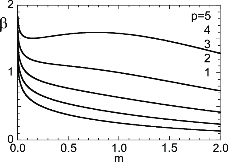
Figure 1: Saddle-point equation (10) in the canonical ensemble at $d=2$. The function diverges logarithmically at the origin.

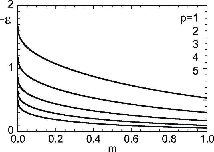
Figure 2: Saddle-point equation (12) in the microcanonical ensemble at $d=2$. The function is finite at the origin.

Let us first write the lattice Green function (6) as, using the variable $m^{2}=2(\tilde{z}-d)$,

$$G(k,\tilde{z})=\frac{2}{m^{2}+\sum_{\mu}\big{(}2\sin(k_{\mu}/2)\big{)}^{2}}.$$ (15)

This is a decreasing function of $m$ and the value at the origin $m=0$ determines the infrared behaviour. When $d=2$, $g(\tilde{z})$ defined in (9) diverges logarithmically at $m=0~{}(\tilde{z}=2)$.

We plot the right-hand sides of (10) and (12) in figures 2 and 2, respectively, for several values of $p$. In the canonical case, the right-hand side of (10) diverges at $\tilde{z}=d=2$ ($m=0$) and is monotonically decreasing when $p\leq 4$. Therefore, in this case, for a given $\beta$, $\tilde{z}$ is determined uniquely. When $p>4$, in a certain range of $\beta$, three solutions exist and $m$ is not determined uniquely. This is understood as the emergence of a first-order transition [25]. On the other hand, the function in (12) for the microcanonical ensemble is finite at the origin ($m=0$) and is a decreasing function for arbitrary $p$. Since the functional value at the origin corresponds to the ground-state energy, the solution is determined uniquely for a given $\epsilon$ larger than or equal to the ground-state energy. Nothing singular happens in this case.

Figure 3: Free energy density $f(T)$ in the canonical ensemble for $d=2$, $p=1$.

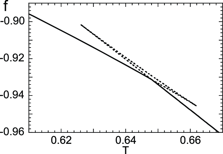
Figure 4: $f(T)$ in the canonical ensemble for $d=2$, $p=5$. The dotted line denotes the thermodynamically irrelevant (unstable or metastable) saddle-point solutions.

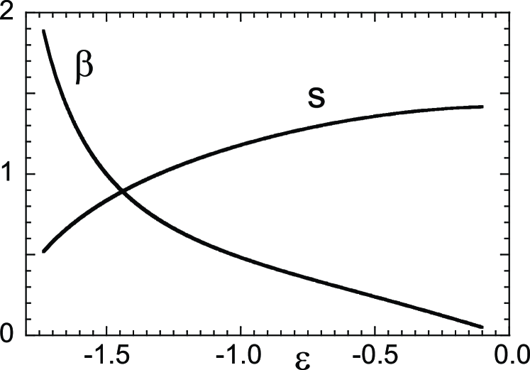
Figure 5: Entropy density $s(\epsilon)$ and inverse temperature $\beta(\epsilon)=ds(\epsilon)/d\epsilon$ in the microcanonical ensemble for $d=2$, $p=1$.

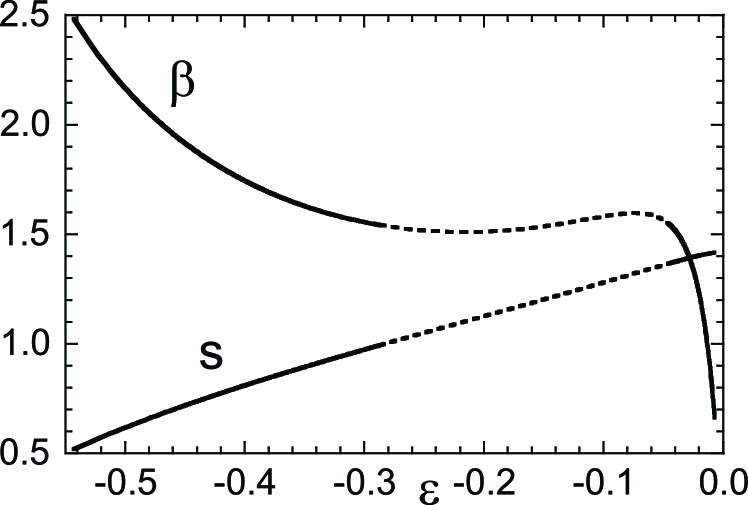
Figure 6: $s(\epsilon)$ and $\beta(\epsilon)$ in the microcanonical ensemble for $d=2$, $p=5$. $s(\epsilon)$ is non-concave and correspondingly $\beta(\epsilon)$ is non-monotonic. The dotted parts correspond to the metastable and unstable branches in the canonical ensemble in figure 4.

From the obtained saddle-point solution in the canonical ensemble, we plot the free-energy density $f$ for $p=1$ and 5 in figures 4 and 4, respectively. We see that a first-order transition occurs when $p=5$. We also plot the entropy density $s$ and the inverse temperature $\beta=ds/d\epsilon$ in the microcanonical ensemble for $p=1$ and 5 in figures 6 and 6, respectively. For $p=5$ in figure 6, we see that $\beta$ is non-monotonic (the entropy is non-concave) for $-0.21<\epsilon<-0.07$ and consequently the specific heat is negative. In this sense, ensembles may seem inequivalent. This behaviour is similar to the case of systems with long-range interactions, where the mean-field picture applies. A remarkable fact is that this mean-field-like behaviour has been found by exact calculations for the two-dimensional system with short-range interactions.

3.3 Phase separation

Ensemble equivalence is recovered in the present system if we choose a proper saddle-point solution which represents a phase-separated state. We have assumed in (13) that the auxiliary variables are independent of the subscripts $i$ and $j$. It implies that the phase is uniform in space. In order to describe the situation with phase separation, we divide the system into two parts with $N_{1}$ and $N_{2}$ spins, respectively. The particular shape of the two sub-regions is not important, as far as they are geometrically compact objects, with a surface-to-volume ratio that vanishes in the thermodynamic limit (for instance, a cubic lattice may be divided into two slabs). We set auxiliary variables in each subsystem as $z^{(1)},\rho^{(1)},\lambda^{(1)}$ and $z^{(2)},\rho^{(2)},\lambda^{(2)}$, respectively. In the thermodynamic limit, we expect that the interface terms between two subsystems are irrelevant due to the short-range nature of the system. We prove it rigorously in B. Then, the number of states $\Omega$ is written as the sum of contributions from two subsystems as

$$\Omega(\epsilon) = \int\frac{dt}{2\pi}\exp\Biggl{[}iNnJt\left\{\epsilon+\frac{N_{1}}{N}dV(\rho^{(1)})+\frac{N_{2}}{N}dV(\rho^{(2)})\right\}$$ (16)

$$+Nn\left(\frac{N_{1}}{N}z^{(1)}+\frac{N_{2}}{N}z^{(2)}\right)-Nn\left(\frac{N_{1}}{N}d\lambda^{(1)}\rho^{(1)}+\frac{N_{2}}{N}d\lambda^{(2)}\rho^{(2)}\right)$$

$$+n\ln\Tr\exp\Biggl{(}-\sum_{i=1}^{N_{1}}z^{(1)}(S_{i}^{(1)})^{2}+\sum_{\langle ij\rangle}\lambda^{(1)}S_{i}^{(1)}S_{j}^{(1)}\Biggr{)}$$

$$+n\ln\Tr\exp\Biggl{(}-\sum_{i=1}^{N_{2}}z^{(2)}(S_{i}^{(2)})^{2}+\sum_{\langle ij\rangle}\lambda^{(2)}S_{i}^{(2)}S_{j}^{(2)}\Biggr{)}\Biggr{]},$$

where $S_{i}^{(1)}$ ($S_{i}^{(2)}$) represents the spin variable in subsystem 1 (2). The saddle-point equations are written as

$$\epsilon=\frac{N_{1}}{N}\epsilon_{1}+\frac{N_{2}}{N}\epsilon_{2},$$ (17)

$$\epsilon_{i}=-dV\left(\frac{\tilde{z}^{(i)}}{d}-\frac{1}{dg(\tilde{z}^{(i)})}\right)\quad(i=1,2),$$ (18)

where $\tilde{z}_{1}=z^{(1)}/\lambda^{(1)}$ and $\tilde{z}_{2}=z^{(2)}/\lambda^{(2)}$. Then, the entropy density is expressed as

$$s=\frac{N_{1}}{N}s_{1}+\frac{N_{2}}{N}s_{2},$$ (19)

$$s_{i}=-\frac{1}{2}\ln g(\tilde{z}^{(i)})-\frac{1}{2}\int\frac{d^{d}k}{(2\pi)^{d}}\ln\left(\tilde{z}^{(i)}-\sum_{\mu=1}^{d}\cos k_{\mu}\right)+\frac{1}{2}+\frac{1}{2}\ln 2\pi.$$ (20)

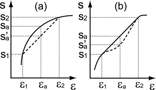
Figure 7: Comparison of the entropies obtained from the uniform and phase-separated solutions. The entropy from the phase-separated solution is represented by the straight lines. (a) When the entropy for the uniform solution is concave, the phase-separated solution is irrelevant because it has a smaller value of the entropy $s^{\prime}_{a}$ than the true $s_{a}$. (b) When the entropy is non-concave, a first-order transition occurs and a phase-separated state is realized between $\epsilon_{1}$ and $\epsilon_{2}$ because it has a larger entropy.

A notable fact is that these expressions hold for any ratio of the separated phases, $c=N_{1}/N,1-c=N_{2}/N$ as well as for any choice of $\epsilon_{1,2}$ and $s_{1,2}$. Thus, we should discuss what values of these parameters are actually chosen for a given fixed value of the energy $\epsilon=\epsilon_{a}$. First, if the total entropy is concave, the hypothetical phase separation means that the value of the entropy would be $s^{\prime}_{a}=cs_{1}+(1-c)s_{2}$, which is lower than the true entropy $s_{a}$ as can be understood from figure 7(a). Thus, there is no phase separation in the stable state. Technically, this means that the exponent of the integral for the number of states $\Omega=e^{S}$ becomes largest at the saddle point representing the uniform state, not at the point corresponding to the phase-separated state.

On the other hand, the situation is different when the total entropy is non-concave as we show in figure 7(b). At $\epsilon=\epsilon_{a}$, the state with the entropy $s=s_{a}=cs_{1}+(1-c)s_{2}$ is more stable than that with $s^{\prime}_{a}$ and is realized as the phase-separated state in the usual sense. Technically, the saddle point corresponding to this former state has the largest contribution to the integral. Thus, we can obtain the phase-separated state by relaxing the uniformity condition of the saddle-point solution. It should be noticed that only the microcanonical solution needs this non-uniform prescription of the saddle-point values. The uniform solution for the canonical case (8) shows no inconsistencies.

3.4 $d=3$

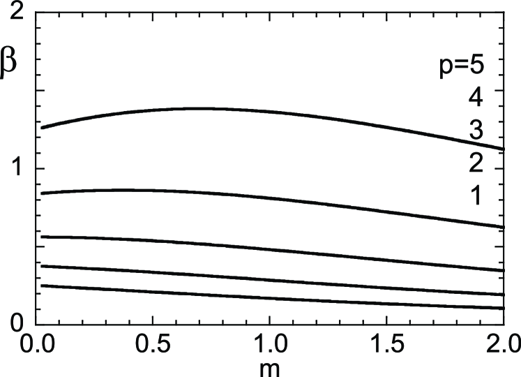
Figure 8: Saddle-point equation (10) in the canonical ensemble at $d=3$.

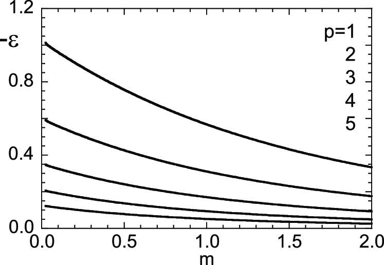
Figure 9: Saddle-point equation (12) in the microcanonical ensemble at $d=3$. The value at the origin is not equal to the ground state energy.

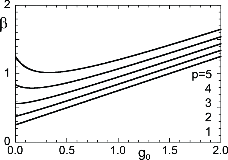
Figure 10: Zero-mode part of the saddle-point equation in the canonical ensemble at $d=3$.

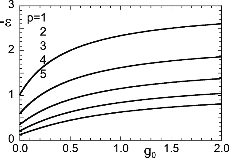
Figure 11: Zero-mode part of the saddle-point equation in the microcanonical ensemble at $d=3$.

Let us next consider the three-dimensional system, in which case $g(\tilde{z})$ is finite at $m=0$ ($g(\tilde{z}=3)\approx 0.505$) and is monotonically decreasing. As shown in figures 9 and 9, the saddle-point equation has no solution at low temperature or low energy. To avoid this difficulty, the zero mode $k=0$ in (9) should be separated from the integral, similarly to the Bose-Einstein condensation, as

$$g(\tilde{z})\to\tilde{g}(k=0,\tilde{z})+g(\tilde{z})=\frac{1}{N}\frac{1}{\tilde{z}-3}+\int\frac{d^{3}k}{(2\pi)^{3}}\frac{1}{\tilde{z}-\sum_{\mu=1}^{3}\cos k_{\mu}}.$$ (21)

The parameter $\tilde{z}$ approaches $3$ in the thermodynamic limit so that the first term gives a finite contribution $g_{0}$ in this limit. Then, we can find the solution of the saddle-point equation by the replacement

$$g(\tilde{z})\to g_{0}+g(3).$$ (22)

As depicted in figures 11 and 11, $g_{0}$ can be fixed from the saddle-point equation for a given $\beta$ (or $\epsilon$) below (or above) the values achievable in figure 9 (or figure 9). Hence, there exists a solution for any $\beta$ or $\epsilon$, the latter being larger than or equal to the ground-state energy.

Figure 12: $f(T)$ in the canonical ensemble for $d=3$, $p=1$. The dot denotes the transition point, where $g_{0}$ starts to be finite.

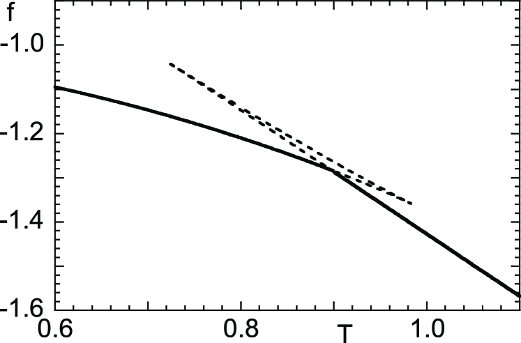
Figure 13: $f(T)$ in the canonical ensemble for $d=3$, $p=5$.

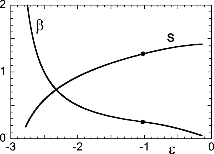
Figure 14: $s(\epsilon)$ and $\beta(\epsilon)$ in the microcanonical ensemble for $d=3$, $p=1$. The dot denotes the transition point.

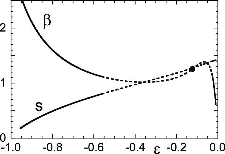
Figure 15: $s(\epsilon)$ and $\beta(\epsilon)$ in the microcanonical ensemble for $d=3$, $p=5$. The putative continuous transition point denoted by the dot is hidden by a first-order transition. The dotted parts correspond to those in figure 13.

We plot the free energy in the canonical ensemble in figures 13 and 13 for $p=1$ and $p=5$, respectively. A continuous transition to the zero-mode condensed phase is observed for $p=1$. It is replaced by a discontinuous transition for $p=5$. From the microcanonical analysis, we plot $s$ and $\beta$ in figures 15 and 15 for $p=1$ and $p=5$, respectively. As can be understood from these figures, transitions between the condensed and non-condensed phases exist in both ensembles in three dimensions. It is discontinuous for $p=5$. Similarly to the $d=2$ case, the apparent ensemble inequivalence (negative specific heat in the microcanonical ensemble) can be avoided by the proper choice of the saddle-point solution.

4 Monte Carlo analysis

In order to check if the results of the previous section is specific to the spherical model, we study the $n=2$ model, the $XY$ model, in two dimensions by Monte Carlo simulations. A canonical Monte Carlo analysis of the present model has already been carried out in [23], and the microcanonical case has been done in [33]. However, these previous studies are not sufficient to clarify the problem of ensemble equivalence, and we analyze the same model here from our own point of view. We refer the reader to [34] for a related study, where the ensemble equivalence was examined in a mean-field model on random graphs.

The original $XY$ model with linear interactions in two dimensions exhibits the Kosterlitz-Thouless transition [35]. In [36], a detailed study is reported on how the transition can be changed in nonlinearly-interacting systems. Since our aim is not to study this topological transition, only the caloric curve has been calculated in our Monte Carlo analysis.

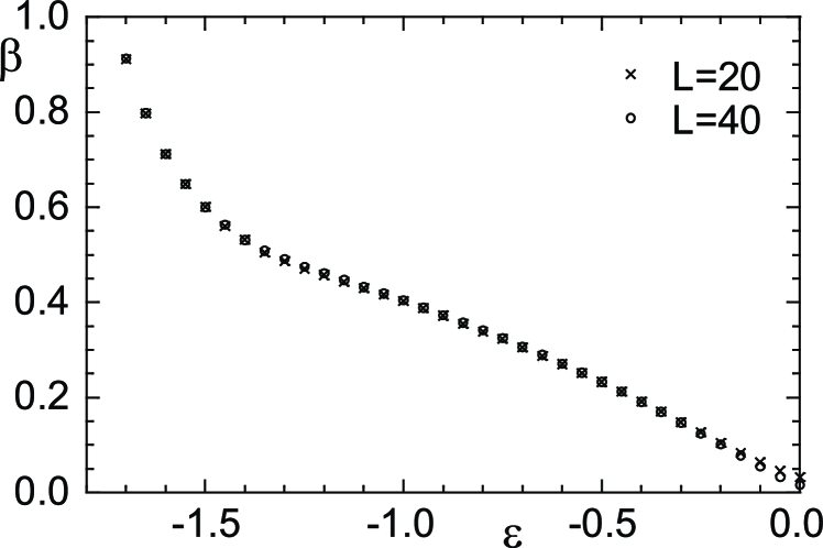
Figure 16: $\beta(\epsilon)$ from the microcanonical Monte Carlo calculation for $n=2$, $d=2$ and $p=1$. The error bars are smaller than the symbol size.

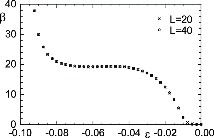
Figure 17: $\beta(\epsilon)$ for $n=2$, $d=2$ and $p=40$. The error bars are smaller than the symbol size.

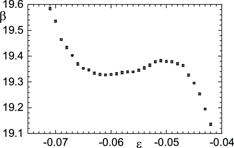
Figure 18: $\beta(\epsilon)$ for $n=2$, $d=2$, $p=40$, and $L=50$ near the non-monotonic region. We have taken the average over 20 independent runs.

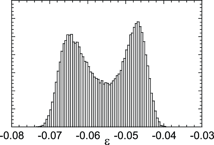
Figure 19: Energy histogram in the phase coexistence region from the canonical Monte Carlo calculation. We have chosen $n=2$, $d=2$, $p=40$, $L=50$, and $\beta=19.35$.

Several system sizes have been analyzed, $L=20$, 40, 50 and larger in some cases. To study the microcanonical ensemble, we exploit the demon algorithm by Creutz [32]. In this algorithm, for a given energy $\epsilon$, the demon energy $E_{\rm D}$ is calculated so that the sum of the system and demon energies is kept constant. Then, the inverse temperature is obtained from the probability distribution ${\rm Prob}(E_{\rm D})\sim\exp(-\beta E_{\rm D})$. We have performed $10^{6}$ Monte Carlo steps per spin for each run.

In figures 17 and 17, we plot the energy dependence of the inverse temperature for $p=1$ and $p=40$, respectively. For $p=1$, we see that $\beta$ is a monotonically decreasing function of $\epsilon$. It is different for $p=40$, where the function shows a non-monotonic behaviour. Figure 19 highlights this property for $L=50$. For a given $\beta$, $\epsilon$ is not determined uniquely in a narrow region, which suggests the existence of negative specific heat. We have performed canonical Monte Carlo calculations using the simple Metropolis algorithm to see the energy histogram, and the result is depicted in figure 19, which clearly shows that a first-order transition exists in the form of phase coexistence. We have confirmed that the non-monotonic region of the caloric curve remains up to the size $L=100$ in the microcanonical simulations. An extrapolation suggests that it would persist to the thermodynamic limit. Thus, the negative specific heat seems to exist in the microcanonical ensemble also in the two-component system as in the spherical model.

We speculate that a reason for the apparent ensemble inequivalence for $p=40$ in Monte Carlo simulations may be that a phase separation, as discussed above for the spherical model, has not been realized in our simulations because of a very long relaxation time: The system has to spontaneously break up into two spatially separated regions with different macroscopic states, which could take a very long time to be realized in the microcanonical simulations.

5 Summary and conclusion

We have studied the $n$-vector model ($O(n)$-symmetric model) with nonlinear short-range interactions in two and three dimensions. The exact solution of the spherical model shows ostensible inequivalence of canonical and microcanonical ensembles through negative specific heat in the latter ensemble. We have argued that this paradox can be resolved by explicitly taking into account a phase separation, which increases the entropy (thus increases the thermodynamic stability) in the microcanonical ensemble. It is noticed that the proper choice of the saddle-point solution is required in the microcanonical ensemble to represent the state with phase separation. Such a solution must be considered when the uniform ansatz of the saddle-point solution gives a non-concave entropy. We note that this procedure is needed only in the microcanonical ensemble. In the canonical ensemble, the uniform solution is sufficient to represent the stable state of the system. Another interesting aspect is that the exact solution of the spherical model is similar to the mean-field solutions applicable to long-range interacting models in the sense that the calculations of the (canonical) partition function and the (microcanonical) entropy reduced to steepest descent integrations. The difference between the short- and long-range systems is apparent when we consider the phase-separated state. The interface term cannot be neglected in the long-range system, which can be understood as an important source of ensemble inequivalence. Our analysis has succeeded to highlight this difference in an exactly solvable example.

The $XY$ model with nonlinear interactions has been shown to behave similarly by Monte Carlo simulations in two dimensions. Discrepancies between ensembles may in this case be due to the long relaxation time to the fully-stable phase-separated state in the microcanonical simulation. We expect that a more elaborate method such as the one developed in [37] may resolve this problem.

The $n$-vector models with nonlinear short-range interactions have been known to have the unusual property of the existence of first-order phase transitions even in two (and higher) dimensions [23]-[27]. We have identified an additional highly non-trivial property of apparent ensemble inequivalence, which we expect to stimulate further studies of this very unusual class of models.

Appendix A Derivation of the entropy in the microcanonical ensemble

We consider the number of states for a given energy $E$

$$\Omega=\Tr\delta(E-H)=\int\frac{dt}{2\pi}\Tr e^{i(E-H)t}.$$ (23)

This expression has a similar form to the partition function in the canonical ensemble except for the integral over $t$ and the factor $e^{iEt}$. We may thus replace $\beta$ in the partition function by $it$. Therefore, the calculation goes along the same line as in the canonical case and we can write

$$\Omega = \int\frac{dt}{2\pi}\int\prod_{i}dz_{i}\prod_{\langle ij\rangle}d\lambda_{ij}d\rho_{ij}\,\exp\left[it\Biggl{(}E+Jn\sum_{\langle ij\rangle}V\left(\rho_{ij}\right)\Biggr{)}+n\sum_{i=1}^{N}z_{i}\right.$$ (24)

$$\left.-n\sum_{\langle ij\rangle}\lambda_{ij}\rho_{ij}+n\ln\Tr\exp\left(-\sum_{i=1}^{N}z_{i}S_{i}^{2}+\sum_{\langle ij\rangle}\lambda_{ij}S_{i}S_{j}\right)\right].$$

Then, we impose the uniform ansatz for $z_{i}$, $\rho_{ij}$ and $\lambda_{ij}$ and obtain the number of states as

$$\Omega = \exp\Bigg{[}it\Bigl{(}E+NndJV(\rho)\Bigr{)}+Nnz-Nnd\lambda\rho$$ (25)

$$+n\ln\Tr\exp\Biggl{(}-\sum_{i=1}^{N}zS_{i}^{2}+\sum_{\langle ij\rangle}\lambda S_{i}S_{j}\Biggr{)}\Biggr{]},$$

and the saddle-point conditions

$$\epsilon+dV(\rho)=0,\quad\lambda=itJV^{\prime}(\rho),\quad 2\lambda=g(\tilde{z}),\quad d\rho=\tilde{z}-\frac{1}{2\lambda},$$ (26)

where $\epsilon=E/NnJ$. Combining these results, we finally obtain (12) and (14).

Appendix B Bounds on interface effects in the free energy of the Gaussian model

In order to rigorously justify the calculations using only the two phase-separated regions without interface terms, let us estimate the order of magnitude of the effects that the interface terms have on the free energy of the Gaussian model. We define the free energy of the Gaussian model as

$$h(x)=\ln\Tr\exp\left(-z\sum_{i}S_{i}^{2}+\lambda\sum_{\langle ij\rangle}^{(1)}S_{i}S_{j}+\lambda x\sum_{\langle ij\rangle}^{(2)}S_{i}S_{j}\right),$$ (27)

where the summation with superscript (1) runs over all interactions within the two independent (phase-separated) subsystems and the summation with superscript (2) is for interactions across the interface. The parameter $\lambda$ will be assumed to be positive without losing generality on a bipartite lattice. Notice that we have assumed that the interactions have common values in the two subsystems. We will show later that this restriction can be removed. The boundary conditions are assumed to be free in the $x$ direction and periodic otherwise. Here the term ‘interface’ stands for the region in the middle of the system that runs perpendicular to the $x$ axis and separates two subsystems, whereas the ‘boundary’ is for the outmost sites of the total system. Equation (27) indicates that the interface interactions have the strength $\lambda x$ and all other interactions have $\lambda$.

Our goal is to prove that

$$|h(1)-h(0)|\leq cN_{b},$$ (28)

where $N_{b}$ is the number of interactions across the interface and $c$ is a quantity asymptotically independent of $N_{b}$ and $N$ (total number of sites). This inequality (28) shows that the presence and absence of boundary interactions affect the free energy only by a term proportional to $N_{b}$ and thus can be neglected in the thermodynamic limit where the leading term is of order $N$.

Let us first notice that the derivative of $h(x)$ is non-negative, the first Griffiths inequality,

$$h^{\prime}(x)=\lambda\frac{\Tr\sum_{\langle ij\rangle}^{(2)}S_{i}S_{j}e^{-H(x)}}{\Tr e^{-H(x)}}\geq 0,$$ (29)

where $-H(x)$ is the effective Hamiltonian appearing in the exponent of (27). The denominator of (29) is positive. The numerator is also non-negative for $0\leq x\leq 1$: Each term of the expansion of the numerator

$$\Tr\sum_{\langle ij\rangle}^{(2)}S_{i}S_{j}\sum_{n=0}^{\infty}\frac{\lambda^{n}}{n!}\left(\sum_{\langle ij\rangle}^{(1)}S_{i}S_{j}+x\sum_{\langle ij\rangle}^{(2)}S_{i}S_{j}\right)^{n}e^{-z\sum_{i}S_{i}^{2}}$$ (30)

is composed of integrals of the form

$$\Tr S_{i}^{a}S_{j}^{b}S_{k}^{c}\,e^{-z\sum S_{i}^{2}},$$ (31)

which is zero (if any one of $a,b,c,\cdots$ is odd) or positive (otherwise). The second derivative is also non-negative:

$$h^{\prime\prime}(x)=\lambda^{2}\left[\left\langle\left(\sum_{\langle ij\rangle}^{(2)}S_{i}S_{j}\right)^{2}\right\rangle_{\rm G}-\left(\left\langle\sum_{\langle ij\rangle}^{(2)}S_{i}S_{j}\right\rangle_{\rm G}\right)^{2}\right]\geq 0,$$ (32)

where $\langle\cdots\rangle_{\rm G}$ stands for the average by the weight $e^{-H(x)}$. Thus $h^{\prime}(x)$ is non-decreasing and is bounded by $h^{\prime}(1)(\geq 0)$ for $0\leq x\leq 1$. Therefore

$$|h(1)-h(0)|=\left|\int_{0}^{1}dx\frac{dh}{dx}\right|\leq\int_{0}^{1}dx\left|\frac{dh}{dx}\right|\leq h^{\prime}(1).$$ (33)

Our task is to upper-bound $h^{\prime}(1)$. From the definition of $h(x)$, this derivative is expressed as

$$h^{\prime}(1)=\lambda N_{b}\langle S_{i}S_{j}\rangle_{\rm G}(x=1),$$ (34)

where $\langle ij\rangle$ is a bond across the interface. According to (33), if we are able to prove that $\langle S_{i}S_{j}\rangle_{\rm G}(x=1)$ is finite in the thermodynamic limit ($N\to\infty,N_{b}\to\infty$), we will have finished the proof that $h(1)$ and $h(0)$ are no more different than a quantity of order $N_{b}$. This implies that the contribution of the interface interactions can be neglected in the computation of the bulk free energy.

Finiteness of $r(y=0)\equiv\langle S_{i}S_{j}\rangle_{\rm G}(x=1)$ can be shown as follows. The argument $y$ of $r(y)$ stands for the strength of interactions connecting the left-most sites and right-most sites along the $x$ direction. In other words, $y=1$ corresponds to the periodic boundary and $y=0$ is for free boundary in the $x$ direction (Remember that $x=1$ ensures that the interactions across the interface exist). All other directions have periodic boundary conditions. The Hamiltonian is modified as

$$-H(x=1,y)=-z\sum_{i}S_{i}^{2}j+\lambda\sum_{\langle ij\rangle}^{(1)}S_{i}S_{j}+\lambda\sum_{\langle ij\rangle}^{(2)}S_{i}S_{j}+y\lambda\sum_{\langle ij\rangle}^{(3)}S_{i}S_{j},$$ (35)

where the final sum with superscript (3) runs over the boundary bonds. Let us assume for the moment that we have proved the following inequality,

$$0\leq r(y=0)\leq r(y=1).$$ (36)

Since $r(1)$ is the single-bond correlation for fully-periodic boundary conditions, we can calculate it explicitly by taking the derivative of the free energy with respect to $\lambda$ and diving the result by the total number of bonds. The explicit form is available for this quantity in (5) and it is easy to see that $r(1)$ is positive and finite provided that $z>d$. This ends the proof that $r(0)$ is finite.

To prove (36), we first notice $r(0)\geq 0$, the first Griffiths inequality, which can be proved as we did above. Next we take the derivative of $r(y)$,

$$r^{\prime}(y)=\lambda\sum_{\langle lm\rangle}^{(3)}\left(\langle S_{i}S_{j}S_{l}S_{m}\rangle_{\rm G}-\langle S_{i}S_{j}\rangle_{\rm G}\langle S_{l}S_{m}\rangle_{\rm G}\right).$$ (37)

The definition of $\langle\cdots\rangle_{\rm G}$ is slightly modified in that the Hamiltonian $-H(x=1,y)$ is now used. Since the integral defining $\langle\cdots\rangle_{\rm G}$ is Gaussian, Wick’s theorem applies,

$$\langle S_{i}S_{j}S_{l}S_{m}\rangle_{\rm G}-\langle S_{i}S_{j}\rangle_{\rm G}\langle S_{l}S_{m}\rangle_{\rm G}$$

$$=\langle S_{i}S_{l}\rangle_{\rm G}\langle S_{j}S_{m}\rangle_{\rm G}+\langle S_{i}S_{m}\rangle_{\rm G}\langle S_{j}S_{l}\rangle_{\rm G}\geq 0,$$ (38)

due to the first Griffiths inequality. The proof of (36) thus completes.

Finally, we show that the result applies also to the case where the two subsystems have different values of $\lambda$. Let us replace $\lambda$ by $u\lambda~{}(0<u\leq 1)$ for one of the two subsystems. The other subsystem keeps the original value of $\lambda$. Then, $r$ is a function of $y$ and $u$. The derivative of $r(y,u)$ with respect to $u$ has an expression very similar to (37), which can be shown to be positive as before. Thus, $r(y,u)\leq r(y,1)$ for $0<u\leq 1$. Since $u=1$ is for the system already treated above, we know that $r(1,1)$ is finite. It then follows that $r(0,u)(\leq r(0,1)\leq r(1,1))$ is finite. All other parts of the proof can trivially be generalized to accommodate $0<u\leq 1$. Q.E.D.

The condition of the outer boundary (free or periodic) along the $x$ axis can also be shown to be irrelevant in the thermodynamic limit. To outline the process, let us define

$$j(y)=\ln\Tr e^{-H(x=1,y)}.$$ (39)

The goal is to prove

$$|j(1)-j(0)|\leq cN_{b},$$ (40)

where $c$ is a quantity that converges to a finite value in the thermodynamic limit and $N_{b}$ is the number of bonds appearing in the summation with superscript (3). To show this, according to our experience above, we should prove the relations

$$j^{\prime}(1)=cN_{b},\quad j^{\prime}(y)\geq 0.$$ (41)

These can be proved in the same manner as before.

References

References

- [1] Ruelle D 1963 Helv. Phys. Acta 36 183
- [2] Lynden-Bell D and Wood R 1968 Mon. Not. R. Astro. Soc. 138 495
- [3] Hertel P and Thirring W 1971 Ann. Phys. 63 520
- [4] Lynden-Bell D and Lynden-Bell R M 1977 Mon. Not. R. Astro. Soc. 181 405
- [5] Posch A H and Thirring W 2005 Phys. Rev. Lett.95 251101
- [6] Posch A H and Thirring W 2006 Phys. Rev.E 74 051103
- [7] Lynden-Bell D and Lynden-Bell R M 2008 Eur. Phys. Lett. 82 43001
- [8] Barré J, Mukamel D and Ruffo S 2001 Phys. Rev. Lett.87 030601
- [9] Ispolatov I and Cohen E G D 2001 Physica A 295 475
- [10] Bouchet F and Barré J 2005 J. Stat. Phys. 118 1073
- [11] Costeniuc M and Ellis R S 2005 J. Math. Phys. 46 063301
- [12] Mukamel D, Ruffo S and Schreiber N 2005 Phys. Rev. Lett.95 240604
- [13] Campa A, Giansanti A, Mukamel D and Ruffo S 2006 Physica A 365 120
- [14] Remírez-Hernández A, Larralde H and Leyvraz F 2008 Phys. Rev. Lett.100 120601
- [15] Remírez-Hernández A, Larralde H and Leyvraz F 2008 Phys. Rev.E 78 061133
- [16] Bouchet F, Dauxois T, Mukamel D and Ruffo S 2008 Phys. Rev.E 77 011125
- [17] Lederhendler A and Mukamel D 2010 Phys. Rev. Lett.105 150602
- [18] Bouchet F, Gupta S and Mukamel D 2010 Physica A 389 4389
- [19] Bertalan Z, Kuma T, Matsuda Y and Nishimori H 2011 J. Stat. Mech. P01016
- [20] Bertalan Z and Nishimori H 2011 Phil. Mag. (published online)
- [21] Campa A, Dauxois T and Ruffo S 2009 Phys. Rep. 480 57
- [22] Schmidt M, Kusche R, Hippler T, Donges J, Kronmüller W, von Issendorff B and Haberland H 2001 Phys. Rev. Lett.86 1191
- [23] Domany E, Schick M and Swendsen R H 1984 Phys. Rev. Lett.52 1535
- [24] Blöte H W J, Guo W and Hilhorst H J 2002 Phys. Rev. Lett.88 047203
- [25] Caracciolo S and Pelissetto A 2002 Phys. Rev.E 66 016120
- [26] van Enter A C D and Shlosman S B 2002 Phys. Rev. Lett.89 285702
- [27] van Enter A C D and Shlosman S B 2005 Commun. Math. Phys. 255 21
- [28] Mussardo G 2010 Statistical Field Theory (Oxford: Oxford University Press)
- [29] Nishimori H and Ortiz G 2011 Elements of Phase Transitions and Critical Phenomena (Oxford: Oxford University Press)
- [30] Behringer H 2005 J. Stat. Mech. P06014
- [31] Kastner M 2009 J. Stat. Mech. P12007
- [32] Creutz M 1983 Phys. Rev. Lett.50 1411
- [33] Ota S and Ota S B 1994 Pramana 43 129
- [34] Barré J and Gonçalves B 2007 Physica A 386 212
- [35] Kosterlitz J M and Thouless D J 1973 J. Phys. C: Solid State Phys.6 1181
- [36] Sinha S and Roy S K 2010 Phys. Rev.E 81 041120
- [37] Martin-Mayor V 2007 Phys. Rev. Lett.98 137207