Dynamics and Bloch oscillations of mobile impurities in one-dimensional quantum liquids

Abstract

We study dynamics of a mobile impurity moving in a one-dimensional quantum liquid. Such an impurity induces a strong non-linear depletion of the liquid around it. The dispersion relation of the combined object, called depleton, is a periodic function of its momentum with the period $2\pi n$, where $n$ is the mean density of the liquid. In the adiabatic approximation a constant external force acting on the impurity leads to the Bloch oscillations of the impurity around a fixed position. Dynamically such oscillations are accompanied by the radiation of energy in the form of phonons. The ensuing energy loss results in the uniform drift of the oscillation center. We derive exact results for the radiation-induced mobility as well as the thermal friction force in terms of the equilibrium dispersion relation of the dressed impurity (depleton). These results show that there is a wide range of external forces where the (drifted) Bloch oscillations exist and may be observed experimentally.

I Introduction

Recent experiments Koehl_PhysRevLett.103.150601 ; Zipkes10 ; Schmid_etal_PhysRevLett.105.133202 ; Wicke_2010arXiv1010.4545W achieved a substantial progress in fabricating and studying dilute impurities immersed in one-dimensional (1d) quantum liquids. Such liquids are formed by ultracold bosonic or fermionic atomic gases placed in 1d optical lattices Moritz_PhysRevLett.91.250402 ; Stoeferle_etal_PhysRevLett.92.130403 ; Fertig_etal_PhysRevLett.94.120403 ; Kinoshita04 ; Kinoshita06 or using the magnetic confinement on atom chips Wicke_2010arXiv1010.4545W . A hyperfine state of a few atoms is then switched locally with the help of the RF magnetic field pulse Koehl_PhysRevLett.103.150601 ; Wicke_2010arXiv1010.4545W . As a result, the atoms become distinguishable from the rest of the quantum liquid and thus may be considered as mobile impurities. Another promising realization is achieved by placing ions of $\mathrm{Yb}^{+}$, $\mathrm{Ba}^{+}$ or $\mathrm{Rb}^{+}$ in the Bose-Einstein condensate of neutral ${}^{87}\mathrm{Rb}$ atoms Zipkes10 ; Schmid_etal_PhysRevLett.105.133202 .

Remarkably, the impurities may be selectively acted upon with the help of external forces. In the case of neutral atoms the external force is gravity, uncompensated by the force from the vertical magnetic trap as the impurity atoms are created in magnetically untrapped states. In the case of an ion, the selective force is due to the applied electric field. These setups thus allow to drive the non-equilibrium dynamics of mobile impurities immersed in a 1d quantum liquid. By releasing the trap after a certain delay time allows monitoring the resulting density and velocity distribution of impurities.

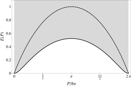
Figure 1: Schematic dispersion relation for a mobile impurity in a weakly interacting superfluid. The dispersion defines the lower bound of the many-particle excitation spectrum. In the region above the dispersion (shaded gray) there exists a continuum of many-body states. The energy is measured in units of the maximum energy of soliton excitations in the superfluid background, shown by the dashed line.

It is important to emphasize that in this publication we are dealing with the case of impurities with finite bare mass $M$, not very different from the mass $m$ of the particles in the background. The velocity of the impurity is therefore free to change as a result of absorbed momentum. This situation is qualitatively different from that of static, infinitely massive impurities Kane_Fisher_PhysRevB.46.15233 ; Hakim_PhysRevE.55.2835 ; Buechler_Geshkenbein_Blatter_2001 ; Astrakharchik2004Motion .

Dynamics of mobile impurities in quantum liquids is an old subject pioneered by Landau and Khalatnikov LandauKhalatnikov1949ViscosityI ; LandauKhalatnikov1949ViscosityII and Bardeen, Baym, Pines and Ebner Bardeen_etal_PhysRevLett.17.372 ; *Bardeen_etal_PhysRev.156.207; *Baym_PhysRevLett.17.952; *Baym_PhysRevLett.18.71; *Ebner_PhysRev.156.222; BaymEbner1967Phonon in their studies of ${}^{3}\mathrm{He}$ atoms in superfluid ${}^{4}\mathrm{He}$. These authors realized that at a finite temperature the impurities experience a viscous force from the normal component of the liquid, even if their speed is less than the critical superfluid velocity. The mechanism leading to such a viscous force was shown to be the Raman scattering of the thermal excitations of the superfluid i.e. thermal phonons scattering off the impurity ${}^{3}\mathrm{He}$ atoms. It was found LandauKhalatnikov1949ViscosityI ; *LandauKhalatnikov1949ViscosityII; BaymEbner1967Phonon that the corresponding friction coefficient scales with temperature as $T^{8}$ in the low temperature limit. It was later discussed by Castro-Neto and Fisher castro96 that in 1d the Raman mechanism leads to the friction force proportional to $T^{4}$ due to the phase-space considerations. The same mechanism governs the temperature-induced acceleration of grey solitons Muryshev2002Dynamics . Recently, two of the present authors Gangardt09 ; Gangardt2010Quantum showed that in addition to phase-space effects the friction is extremely sensitive to the details of the interactions between impurity and the background liquid and vanishes for exactly solvable 1d models. The friction therefore may be rather small in the spin-flip setup if the parameters are near the Yang-Gaudin CN_Yang_1967 ; *Gaudin_1967 integrable case.

Due to the one-dimensional kinematics the slowly moving impurity tends to deplete the host liquid creating density and current gradients in its vicinity. At small momenta the dispersion of the impurity can still be described by quadratic law $E=P^{2}/2M^{*}$ with effective mass $M^{*}$ of the impurity atom Fuchs_2005 ; Matveev08 . In the weakly interacting regime and sufficiently small momenta the depletion of the host liquid can be studied within the framework of Bogoliubov theory. The resulting excitations, polarons, consist of impurities surrounded by a cloud of linear excitations of the condensate and were studied in Ref. Lee_Gunn_PhysRevB.46.301 and later in Refs. Cucchietti_Timmermans_PhysRevLett.96.210401 ; Bruderer_etal_PhysRevA.76.011605 . However, even for a weakly interacting liquid, the induced depletion becomes essentially non-linear at larger momenta and/or strong impurity-liquid coupling. This brings a qualitative change of the dispersion relation and we introduce a quasiparticle which we call depleton describing the impurity dressed by the non-linear depletion cloud.

The remarkable property of depleton dispersion is that it is a periodic function of the momentum $P$ with the period $2\pi\hbar n$, where $n$ is the density of 1d host liquid. To explain this feature it is worth noticing that, being quadratic at small momenta, the depleton energy is less than any of the excitations of the host liquid (see Fig. 1). Indeed, the low-energy excitations of the host liquid have a sound-like nature with the energy $cP>P^{2}/2M^{*}$, where $c$ is the speed of sound. Therefore the dressed impurity excitation provides the cheapest way for the system to accommodate a small momentum. This means that the depleton dispersion relation is defined as the lowest possible many-body excitation energy of the system with a given momentum. An example of such dispersion is shown in Fig. 1. Above the depleton energy there is a continuum of many-body excitations comprised of the moving impurity and a certain number of phonons. This spectral edge is characterized by the power-low singularities of zero-temperature correlation functions and was discussed in Refs. zvonarev_2007 ; Kamenev08 ; Matveev08 ; Zvonarev_etal_PhysRevB.80.201102 .

One may argue now that in the infinite system the ground-state energy with a given momentum is a periodic function of the latter with the period $2\pi\hbar n$. Indeed, it is easy to see that the ground-state energy with momentum $2\pi\hbar n$ vanishes in the thermodynamic limit. To this end consider a ring of length $L$ where the spectrum of the momentum operator is quantized in units of $2\pi\hbar/L$. If the momentum of each particle is boosted by one quantized unit, the total momentum of the system is $2\pi\hbar n$, while the total energy vanishes thanks to the total mass diverging in the thermodynamic limit. We thus conclude that the ground-state for a given momentum $P$ which is the dispersion relation $E(P)$ of the dressed impurity is a periodic function of momentum. Explicit examples are provided by exactly solvable models zvonarev_2007 and weakly interacting Bose-liquid corresponding to Fig. 1 and considered in details in Appendix C.

The physics behind the periodic dispersion relation is in the transfer of momentum from the accelerated impurity to the supercurrent in the background liquid: similarly to the density depletion, the moving impurity creates the sharp phase drop $\Phi$ across it. To satisfy the periodic boundary conditions the rest of the liquid must sustain the phase gradient $\Phi/L$, resulting in the supercurrent which carries momentum $\hbar n\Phi$. While the supercurrent is absorbing momentum, it does not contribute to energy. Indeed, as it was already mentioned, in the thermodynamic limit the bulk of the liquid is infinitely heavy and thus can accommodate any momentum at no energy cost. As a result, the energy and momentum of the depleton core, being periodic functions of the phase drop $\Phi$ with the period $2\pi$, oscillate as functions of the total momentum with the period $2\pi\hbar n$, while the rest of the momentum goes into the supercurrent. A similar periodic dispersion relation would arise if the host liquid were considered as a rigid crystal with the lattice constant $a=1/n$. Then the momentum interval between $P=-\hbar\pi n$ and $P=\hbar\pi n$ is nothing but the Brillouin zone of such a crystal, while the impurity dispersion, discussed above, is its lowest Bloch band.

Although the above considerations completely disregard the absence of the true long-range order in the 1d liquid (either superfluid or crystalline) and thus should be taken with care, the periodicity of the dispersion suggests the possibility of Bloch oscillations of the impurity atom subject to an external force Gangardt09 . Indeed, if an external force $F$ is applied to the impurity atom (e.g. electric field is acting on an ion) the total momentum of the system changes linearly with time, $P=Ft$. For infinitesimal force this leads to adiabatic change of the energy $E(P)$ and the velocity $V=\partial E/\partial P$ of the depleton which become periodic functions of time with the period $2\pi\hbar n/F$. It is quite remarkable that in such a process, on average, the impurity does not accelerate; moreover, it does not even move. Instead, it channels the momentum into the collective motion, i.e., the supercurrent, of the liquid and in the process oscillates around a fixed location. As a result, no energy is transferred, on average, to the system from the external potential.

This spectacular phenomenon is present at zero temperature and under an infinitesimal external force. Both finite temperature and a finite force complicate the picture in a substantial way. The aim of this paper is to clarify the influence of these two factors on the observability of the Bloch oscillations. In brief, our conclusions are as follows: at a sufficiently low temperature there is a parametrically wide range of external forces $F_{\mathrm{min}}(T)<F<F_{\mathrm{max}}$, where the Bloch oscillations are observable. Contrary to the adiabatic picture, they are accompanied by a drift and exhibit certain amplitude and period renormalization.

The drift manifests itself in the appearance of an average velocity $V_{D}$, superimposed on top of the periodic Bloch oscillations. It is a linear function of force at small forces, allowing to define the impurity mobility $\sigma$, as $V_{D}=\sigma F$. As a result, the total energy of the system increases (i.e. the system is heated) with the rate $FV_{D}=\sigma F^{2}$. This energy goes to the emitted long wavelength phonons, which run away from the impurity with the sound velocity $c$. The maximal force can then be estimated as $F_{\mathrm{\max}}\approx c/\sigma$. At a larger force the drift velocity exceeds $c$, leading to Cherenkov radiation of phonons. The phonons take a substantial part of the momentum and thus ruin the Bloch oscillation mechanism, discussed above. The impurity motion is then either incoherent drift, or an unlimited acceleration, depending on the parameters.

We derive the exact analytic expression for the drift mobility $\sigma$ expressed in terms of the equilibrium dispersion relation of the impurity. It is worth noticing that the mobility $\sigma$ is not the linear response property, despite the linear relation between the drift velocity and the external force. Indeed, the dynamics of depleton in this regime is the drift superimposed with the essentially non-linear pattern of Bloch oscillations in which the particle explores the entire range of impurity momenta and energy. It is therefore not immediately obvious that the mobility $\sigma$ may be expressed in terms of the equilibrium properties. Nevertheless we prove that such a relation does exist.

The true linear response is associated with the thermally induced Landau-Khalatnikov friction force $F_{\mathrm{fr}}(V)\propto-T^{4}V$, which arises due to the Raman scattering of phonons discussed above. It provides the lower limitation on the externally applied force $F_{\mathrm{min}}(T)=F_{\mathrm{fr}}(V_{c})$, where $V_{c}$ is the maximal equilibrium velocity given by the maximum slope of the depleton dispersion, Fig. 1. Indeed, at smaller external forces the velocity saturates and therefore the depleton dynamics is confined to the small momenta and Bloch oscillations do not occur.

The friction coefficient in the small momentum regime was discussed in Ref. Gangardt09 and found to be vanishing in exactly solvable cases. The reason behind it is the presence of infinite number of the conservation laws, which prevent a non-equilibrium state from thermalization. Here we extend those calculations to the case where the impurity explores the entire range of momenta and derive an exact result for the full momentum dependence of the friction force. Quite naturally, it vanishes in exactly solvable cases too.

The outline of the paper is as follows: in Section II we give a qualitative description of the depleton quasiparticles and the mechanism of coupling to linear sound excitations, or phonons, of the background liquid. Section III is devoted to the formal derivation of the depleton Lagrangian based on superfluid thermodynamics. We discuss coupling of the depleton with the phonon subsystem and derive a set of stochastic equations of motion for the impurity dynamics in Section IV. These equation are then used to study radiation losses and derive expression of depleton mobility in Section V and thermal friction in Section VI. The main results are summarized in Section VII. Technical details are delegated to Appendices.

II Qualitative analysis

The key to understanding the impurity dynamics is in its interactions with the phonons of the host liquid. This problem is rather non-trivial even if the impurity is weakly coupled to the liquid. Indeed, no matter how weak the interactions are, the impurity develops local depletion, which become appreciable when the impurity momentum approaches $\pi n$ (we set $\hbar=1$ throughout the rest of the paper). To visualize this process it is useful to assume a semiclassical picture of the background, valid for weakly interacting Bose liquid. In this regime, to accommodate the total momentum $\pi n$ the depletion cloud takes the form of the dark soliton Tsuzuki_1971 . The dark soliton is an essentially non-linear mesoscopic object, which includes a large number of particles and a complete depletion of the liquid density. It is exactly the soliton formation which is responsible for channeling momentum into the supercurrent and thus for the Bloch oscillations. It is also the soliton which determines the interactions of the impurity with the dynamically induced phonons. Therefore the non-equilibrium dynamics of the quantum impurity cannot be separated from the dynamics of the essentially non-linear soliton-like depletion cloud.

What makes the problem analytically tractable is the scale separation between the spatial extent of the local soliton-like cloud and the characteristic phonon wavelength. The former is given by the healing length $\xi=1/mc$. The latter appears to be much longer than $\xi$, if the temperature is sufficiently low and the external force is not too strong. One can thus separate the near-field mesoscopic region, which contains the quantum impurity and its depletion cloud, from the far-field region, supporting the radiation emitted by the impurity. Since the depletion is restored exponentially at the healing length away from the impurity, the precise position of the boundary between the near-field and the far-field regions is of no importance.

Because of the wide difference in their spatial scales, the impurity together with its entire non-linear depletion cloud represents a dynamic point-like scatterer for the long wavelength phonons. From the viewpoint of such phonons any point scatterer may be entirely described by two phase shifts. These two phase shifts are the discontinuities of the phonon displacement and momentum fields across the scatterer. They may be expressed through the number of depleted particles $N$ and the phase drop $\Phi$ across the depleton quasiparticle. Therefore out of many degrees of freedom of the near-field region only $N$ and $\Phi$ interact with the phononic sub-system.

What remains is to describe the dynamics of the local depletion cloud with certain fixed values of $N$ and $\Phi$. Solution of this latter problem is facilitated by the fact that the characteristic equilibration rate of the cloud, estimated as $1/\tau=c/\xi$, is much faster than the relevant phononic frequencies. As a result, the cloud may be treated as being in the state of local equilibrium, conditioned to certain values of the slow collective coordinates $N$ and $\Phi$. The fact that there are two such slow variables is due to the presence of the two conservation laws: number of particles and momentum. The fast internal equilibration of the near-field region is therefore conditioned by the instantaneous values of the two conserved quantities.

The slow change (compared to the fast time scale of $\tau$) in the number of depleted particles $N$ and the phase drop $\Phi$ are due to the fact that the local chemical potential $\mu$ and the local current $j$ at the position of the impurity are both affected by the state of the global phononic sub-system. As a result, one may express the Lagrangian of the near-field region as a function of $N$ and $\Phi$ through the equilibrium thermodynamic potential which is a function of $\mu$ and $j$. This latter function may be independently measured or analytically evaluated in certain limiting cases and for exactly solvable models.

These considerations allow one to separate the local, non-linear but equilibrium problem, from the global, non-equilibrium but linear one. The latter statement implies that the host liquid sufficiently far away from the impurity may be treated as the linear i.e. Luttinger liquid PopovBookFunctional ; HaldanePRL81 . This is certainly an approximation which disregards the possibility of the moving impurity to emit non-linear excitations, such as grey solitons or shock waves. The train of solitons emitted by the impurity moving with a constant supercritical velocity was indeed observed in simulations of Ref. Hakim_PhysRevE.55.2835 . The kinematics of this process suggests that it is only possible if the drift velocity is close to the speed of sound $c$. We therefore assume that as long as $F<F_{\mathrm{max}}$, one may disregard solitons emission and treat the liquid away from the impurity as the linear one. This is essentially the same criterion, which allows us to separate the depletion cloud from the long wavelength phonons.

Adopting these approximations, one is able to integrate out the phononic degrees of freedom, characterizing the liquid away from the impurity. It reduces the problem to the dynamics of the impurity described by its coordinate $X(t)$ and momentum $P(t)$ along with the dynamics of its near-field depletion cloud fully described by the two collective coordinates i.e. number of depleted particles $N(t)$ and the phase drop $\Phi(t)$. We derive an effective action written in terms of such an extended set of degrees of freedom. Such an action leads to the coupled system of quantum Langevin equations governing the dynamics of the depleton.

Away from equilibrium, for $F>F_{\mathrm{min}}$, the equations of motion yield the pattern of Bloch oscillations. The deterministic part of these equations provides with the information about drift velocity, amplitude and shape of the velocity oscillations, as well as their period. The stochastic part results in a certain dephasing of the oscillations. It is interesting to notice that the stochastic part is manifestly different from the equilibrium noise, prescribed by the fluctuation-dissipation theorem. As a consequence, the exactly integrable models loose their special status and their non-equilibrium dynamics appears to be not qualitatively different from the dynamics of generic non-integrable models.

III Lagrangian of the mobile impurity

Let us first consider the background liquid in the absence of impurity employing hydrodynamical description proposed by Popov PopovBookFunctional . Its Lagrangian is expressed in terms of the slowly varying chemical potential $\mu$ and density $n$ as an integral of the local thermodynamic pressure

$$L_{0}(\mu,n)=\int\!dx\,p_{0}(\mu,n)=\int\!dx\,\Big{[}\mu n-e_{0}(n)\Big{]}.$$ (1)

Here $e_{0}(n)$ is the energy density of the liquid. In the thermodynamic equilibrium the density is a function of the chemical potential, given by a solution of the following equation: $\mu=\mu(n)=\partial e_{0}/\partial n$, which is a result of the minimization of this functional with respect to $n$. This way one defines the grandcanonical thermodynamic potential of the host liquid as

$$\Omega_{0}(\mu)=-L_{0}(\mu,n(\mu))\,.$$ (2)

For a uniform system the Lagrangian and the corresponding thermodynamic potential are both proportional to the length of the system.

Consider now an impurity of mass $M$, having a coordinate $X$ and moving through the liquid with velocity $V=\dot{X}$, as measured in the laboratory reference frame. It is convenient to choose the reference frame where the impurity is at rest and the liquid flows with the velocity $-V$, as shown in Fig. 2. In this co-moving frame the impurity experiences the supercurrent $j^{\prime}$ and the chemical potential $\mu^{\prime}$. Hereafter primes denote physical quantities defined in the co-moving frame to distinguish them from the corresponding quantities in the laboratory frame. We employ Galilean transformation into the moving frame which gives

$$j^{\prime}=-nV,\qquad\mu^{\prime}=\mu+mV^{2}/2.$$ (3)

Together with the Galilean transformation of the energy density $e^{\prime}_{0}=e_{0}+mV^{2}/2$, the transformation (3) combined with Eqs. (1) and (2) show the invariance of the background grandcanonical potential $\Omega^{\prime}_{0}(\mu^{\prime})=\Omega_{0}(\mu)$. As expected from the Galilean invariance, the latter is independent of the velocity $V$ or the supercurrent $j^{\prime}$.

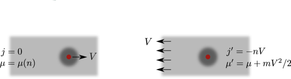
Figure 2: Transformation to moving frame.

We introduce now the impurity into the flowing liquid maintaining both $j^{\prime}$ and $\mu^{\prime}$ fixed and let it equilibrate. Its motion distorts the host liquid density and velocity fields, forming the depletion cloud moving along with the impurity. The grandcanonical potential increases by an amount $\Omega^{\prime}_{\mathrm{d}}(j^{\prime},\mu^{\prime})=E^{\prime}_{\mathrm{d}}-\mu^{\prime}N_{\mathrm{d}}$, where $E^{\prime}_{\mathrm{d}}$ and $N_{\mathrm{d}}$ are the corresponding changes in energy and number of particles. Using the Galilean invariance one can relate the energy $E^{\prime}_{\mathrm{d}}=E_{\mathrm{d}}-P_{\mathrm{d}}V+mN_{\mathrm{d}}V^{2}/2$ to the energy $E_{\mathrm{d}}$ and momentum $P_{\mathrm{d}}$ induced by the moving impurity in the laboratory frame. This fact and relations (3) allows one to identify, in the spirit of Popov’s approach, the Lagrangian of the depletion cloud with the negative change of the grandcanonical potential

$$L_{\mathrm{d}}(V,n) = P_{\mathrm{d}}V-E_{\mathrm{d}}+\mu N_{\mathrm{d}}=-E^{\prime}_{\mathrm{d}}+\mu^{\prime}N_{\mathrm{d}}=-\Omega^{\prime}_{\mathrm{d}}(j^{\prime},\mu^{\prime})\,.$$ (4)

This relation is quite remarkable as the left hand side describes dynamics of the polarization cloud moving with the velocity $V$, while its right hand side is the thermodynamic quantity. The link between them comes from the Galilean transformation, Eqs. (3). The relation between the Lagrangian and the grandcanonical potential, Eq. (4), can be viewed as a generalization of the Popov relation, Eq. (2), to the case of mobile impurities.

Two remarks are in order. First, in assuming the thermodynamic equilibrium at nonzero supercurrent $j^{\prime}$ flowing through the impurity we rely on the superfluidity. Second, we note that the increase in energy $E^{\prime}_{\mathrm{d}}$, momentum $P_{\mathrm{d}}$, number of particles $N_{\mathrm{d}}$ and the grandcanonical potential $\Omega^{\prime}_{\mathrm{d}}$ due to the presence of one single impurity are finite size corrections to the corresponding extensive quantities.

III.1 Collective degrees of freedom of the depleton

Variations of the so far fixed parameters $j^{\prime}$ and $\mu^{\prime}$ of the background liquid induce changes in the thermodynamic potential of the depletion cloud. It can be written with the help of the corresponding response functions as

$$\mathrm{d}\Omega^{\prime}_{\mathrm{d}}=\Phi\,\mathrm{d}j^{\prime}+N\mathrm{d}\mu^{\prime}\,,\qquad\qquad\Phi=\partial_{j^{\prime}}\Omega^{\prime}\,,\;\;\;\;N=\partial_{\mu^{\prime}}\Omega^{\prime}.$$ (5)

The response to the variation of the chemical potential $N=-N_{\mathrm{d}}$ is identified with the number of particles expelled from the liquid by the impurity (hence the minus sign). The response $\Phi$ to the change of the supercurrent $j^{\prime}$ is the superfluid phase and has no analogy in classical thermodynamics. In the state of the global thermodynamic equilibrium both $\Phi$ and $N$ are rigidly locked to $j^{\prime}$ and $\mu^{\prime}$ and, consequently, to $V$ and $n$. This is denoted by writing $\Phi=\Phi_{0}(V,n)$ and $N=N_{0}(V,n)$. These functions can be obtained from the derivatives of the Lagrangian defined in Eq. (4) as described in the next subsection.

In the nonequilibrium situations, where the supercurrent and chemical potential fluctuate it is convenient to treat $\Phi$ and $N$ as independent variables. We perform the standard Legendre transformation to a new thermodynamic potential,

$$H_{\mathrm{d}}(\Phi,N)=\Omega^{\prime}_{\mathrm{d}}-j^{\prime}\Phi-\mu^{\prime}N,\qquad\mathrm{d}H_{\mathrm{d}}=-j^{\prime}\mathrm{d}\Phi-\mu^{\prime}\mathrm{d}N.$$ (6)

The independent variables $\Phi$ and $N$ describe the state of the depleted liquid in the immediate vicinity of the impurity which may or may not be in equilibrium with globally imposed $j^{\prime}$ and $\mu^{\prime}$. In equilibrium situation $H_{\mathrm{d}}(\Phi,N)$ does not contain any additional information with respect to the thermodynamic potential $\Omega^{\prime}_{\mathrm{d}}(j^{\prime},\mu^{\prime})$, which is in turn related to the depletion cloud Lagrangian $L_{\mathrm{d}}(V,n)$ by Eq. (4). The aim of introducing $H_{\mathrm{d}}(\Phi,N)$ is to allow for interactions of the depletion cloud with the long wavelength phonons. As we shall see in Section IV the latter may change the number of particles and the momentum of the depletion cloud, forcing it to equilibrate to some new values of $\Phi$ and $N$. Before turning to phonons, it is instructive to rewrite down the impurity Lagrangian (4) by substituting into it Eq. (6) and considering $\Phi$ and $N$ as independent vaiables,

$$L_{\mathrm{d}}=\frac{1}{2}\,MV^{2}-j^{\prime}\Phi-\mu^{\prime}N-H_{\mathrm{d}}(\Phi,N)\,.$$ (7)

Expressing $j^{\prime}$, $\mu^{\prime}$ through $V$, $n$ using Eq. (3), we finally obtain the Lagrangian of the depleton

$$L(V,\Phi,N)=\frac{1}{2}\,(M-mN)V^{2}+nV\Phi-\mu N-H_{\mathrm{d}}(\Phi,N)\,,$$ (8)

where $\mu=\mu(n)$ is the equilibrium chemical potential of the host liquid in the laboratory frame and we have added the bare kinetic energy proportional to the impurity mass $M$. The momentum of the depleton is obtained by the standard procedure

$$P=\frac{\partial L}{\partial V}=(M-mN)V+n\Phi\,,$$ (9)

The last term describes the supercurrent momentum $n\Phi$ stored in the background. The first term is proportional to the reduced mass $M-mN$, expressing the fact that the mass $mN$ is removed from the local vicinity of the moving impurity. This quantity should not be confused with the effective mass $M^{*}$ given by the curvature the equilibrium dispersion Eq. (15) or obtained from the equilibrium dynamics in Eq. (19).

We can use Eq. (9) to express velocity of the depleton as a function of its momentum,

$$\dot{X}=V=V(P,\Phi,N)=\frac{P-n\Phi}{M-mN}.$$ (10)

Combining Eq. (10) and the Lagrangian (8) leads to the Hamiltonian

$$H(P,\Phi,N) = PV-L=\frac{1}{2}\frac{(P-n\Phi)^{2}}{M-mN}+\mu N+H_{\mathrm{d}}(\Phi,N)\,.$$ (11)

This Hamiltonian generates the following equations of motion

$$\dot{P} = 0$$ (12)

$$0 = -\partial_{\Phi}H=nV-\partial_{\Phi}H_{\mathrm{d}}$$ (13)

$$0 = -\partial_{N}H=-\mu-mV^{2}/2-\partial_{N}H_{\mathrm{d}}$$ (14)

in addition to Eq. (10). The first equation is the momentum conservation expected in the absence of external forces and for homogeneous background. Two other equations are in fact static constraints. This is a manifestation of the already mentioned fact that without phonons $\Phi$ and $N$ are rigidly locked constants and do not have an independent dynamics.

III.2 Dynamics of depleton in the absence of phonons and equilibrium values of collective variables

As we shall see in Section IV, the coordinates canonically conjugated to $\Phi$, $N$ are phononic displacement and phase at the location of the impurity. In the absence of these degrees of freedom the only consistent solution of Eqs. (13), (14) is static relations $\Phi=\Phi_{0}(P,n)$, $N=N_{0}(P,n)$. Substituting them back into the Hamiltonian (11) leads to the equilibrium dispersion relation of the dressed impurity (depleton),

$$H(P,\Phi_{0}(P,n),N_{0}(P,n))=E(P,n)\,.$$ (15)

The corresponding “equilibrium Lagrangian” can be obtained as $L(V,n)=PV-E$ by expressing the momentum with the help of $V=\partial E/\partial P$. In most situations it is rather these quantities and not the “internal energy” $H_{\mathrm{d}}(\Phi,N)$ represent the physical input about the dynamics of the dressed impurity. They can be obtained from solving the equilibrium problem for the impurity moving with the constant momentum $P$ or velocity $V$, through the liquid with the asymptotic density $n$. Below we show explicitly how collective variables $\Phi$ and $N$ and the corresponding energy $H_{\mathrm{d}}$ can be obtained from the knowledge of $E(P,n)$ or $L(V,n)$.

We start with the situation when velocity $V$ is a control parameter. In this case finding $H_{\mathrm{d}}(\Phi,N)$ amounts to perform the Legendre transformation Eq. (6) by exploiting the definition (4) of the Lagrangian $L_{\mathrm{d}}=L-MV^{2}/2$ of the depletion cloud in terms of the thermodynamic potential $\Omega^{\prime}_{\mathrm{d}}$ and using the pair $(V,n)$ instead of the thermodynamical variables $(j^{\prime},\mu^{\prime})$. To achieve this goal we use Eqs. (3) to relate the corresponding partial derivatives by the linear transform

$$\begin{pmatrix}\partial_{V}\\ \partial_{n}\end{pmatrix} = \begin{pmatrix}-n&mV\\ -V&mc^{2}/n\end{pmatrix}\begin{pmatrix}\partial_{j^{\prime}}\\ \partial_{\mu^{\prime}}\end{pmatrix}.$$ (16)

Here we have used the relation $\partial\mu/\partial n=mc^{2}/n$ between the compressibility and the sound velocity $c$. Using the definitions Eqs. (5) and Eqs. (16) we can express the derivatives of $L(V,n)$ in terms of collective variables $\Phi,N$

$$\frac{\partial L}{\partial V}-MV = P-MV=n\Phi-mVN$$ (17)

$$\frac{\partial L}{\partial n} = V\Phi-\frac{mc^{2}}{n}{N}.$$ (18)

Solving these equations yield equilibrium values, $\Phi_{0}(V,n)$ and $N_{0}(V,n)$. Eq. (17) can be otherwise obtained by simply substituting $\Phi_{0}(V,n)$ and $N_{0}(V,n)$ into the definition of the momentum, Eq. (9). This is a consequence of the equations of motion (13), (14). The quantities involving second derivatives of the Lagrangian do not enjoy this property. The most obvious case is the effective mass

$$M^{*}=\frac{\partial P}{\partial V}=M-mN-mV\frac{\partial N_{0}}{\partial V}+n\frac{\partial\Phi_{0}}{\partial V}\,,$$ (19)

which differs from the expression $M-mN$ obtained by taking partial derivative of Eq. (9) with respect to velocity.

The equilibrium relations $\Phi_{0}(V,n)$ and $N_{0}(V,n)$ can be inverted to find velocity $V_{0}(\Phi,N)$, and density $n_{0}(\Phi,N)$ for given values of $\Phi$ and $N$. Substituting them into Eq. (8) gives

$$H_{\mathrm{d}}(\Phi,N)=-L(V_{0},n_{0})+\frac{MV_{0}^{2}}{2}+n_{0}V_{0}\Phi-\left(\mu(n_{0})+\frac{mV_{0}^{2}}{2}\right)N\,.$$ (20)

Conversely, we can use the momentum $P$ as a control parameter. Again, using equations of motion Eqs (13), (14) one is able to show the equivalence of the derivatives $\partial H(P,\Phi,N)/\partial n=\partial E(P,n)/\partial n$ and $\partial H(P,\Phi,N)/\partial P=\partial E(P,n)/\partial P$. The latter defines the velocity $V_{0}(P,n)$. Using these facts and differentiating explicitly Eq. (11) we have the following system of equations

$$V_{0}(P,n)=\frac{P-n\Phi}{M-mN};\,\,\,\,\,\quad\quad\frac{\partial E(P,n)}{\partial n}=\frac{mc^{2}}{n}N-V_{0}(P,n)\Phi,$$ (21)

which are equivalent to Eqs. (17), (18) by virtue of the fact that $(\partial L/\partial n)_{V}=-(\partial E/\partial n)_{P}$. Solving Eqs. (21) yield equilibrium values $\Phi_{0}(P,n)$, $N_{0}(P,n)$ as functions of $P$ and $n$. Next, we invert these relations to obtain $P_{0}(\Phi,N),n_{0}(\Phi,N)$ as functions of $\Phi,N$. Using Eq. (15) and Eq. (11) we obtain the expression for the core energy

$$H_{\mathrm{d}}(\Phi,N)=E(P_{0},n_{0})-\mu(n_{0})N-\frac{1}{2}\frac{(P_{0}-n_{0}\Phi)^{2}}{M-mN}.$$ (22)

in terms of the dispersion $E(P,n)$ and its derivatives.

To illustrate this procedure we use two cases, where the energy $H_{\mathrm{d}}(\Phi,N)$ possesses a simple analytic form. One is the grey soliton in weakly interacting Bose-Einstein condensate describing a massless, $M=0$, impurity propagating in a weakly interacting Bose liquid with the coupling constant $g$. The standard results PitaevskiiStringariBook ; Tsuzuki_1971 for the soliton dynamics are provided in Appendix B and lead to

$$H_{\mathrm{d}}(\Phi,N)=\frac{1}{8}\,mg^{2}N^{3}\left[\frac{1}{3}-\left(\sin\frac{\Phi}{2}\right)^{-2}\right].$$ (23)

Another example is provided by a strongly interacting impurity Castella_Zotos_1993 ; Matveev08 . In this case the number of expelled particles $N$ is almost independent on the state of the impurity and may be considered as a non-dynamic constant. The remaining dependence of energy on the superfluid phase $\Phi$ has a standard Josephson form

$$H_{\mathrm{d}}(\Phi)=-E_{\mathrm{J}}\cos\Phi.$$ (24)

The Josephson energy $E_{\mathrm{J}}=\hbar nV_{\mathrm{c}}$ is expressed through the corresponding critical velocity $V_{\mathrm{c}}$, which in this case is much smaller than the sound velocity $c$.

Expressions (20) or (22) provide the core energy of the locally equilibrium depletion cloud as a function of its slow variables $\Phi$ and $N$. This procedure emphasizes the fact that introduction of $\Phi$ and $N$ does not rely on the semiclassical interpretation of the condensate wavefunction. In fact, they may be defined even away from the semiclassical weakly interacting regime, where the phase of the condensate as well as its depletion are not well defined.

IV Coupling to phonons

An external force $F$ acting on the impurity drives the system away from equilibrium, making the impurity radiate energy and momentum. For a sufficiently weak force such a radiation takes the form of long wavelength phonons, i.e. small deviations of density $\rho(x,t)$ and velocity $u(x,t)$ fields from their equilibrium values, see Fig. 3.

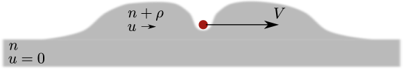
Figure 3: Impurity propagating in local environment.

Below we show how coupling to phonons can be formulated in terms of the collective variables $\Phi,N$. It turns out that this procedure is based solely on the principles of gauge and Galilean invariance, i.e. conservation of number of particles and momentum, and leads to universal results.

IV.1 Hydrodynamic description of phononic bath

We start by considering the Lagrangian, governing dynamics of the phonon fields in the bulk of the liquid. To this end it is convenient to parameterize them by introducing the superfluid phase $\varphi(x,t)$ and the displacement field $\vartheta(x,t)$ such that $u=\partial_{x}\varphi/m$ and $\rho=\partial_{x}\vartheta/\pi$. The dynamics of these variables can be described following the method of Popov PopovBookFunctional by considering slow change of the density $n\to n+\rho(x,t)$ and, independently, the change of the chemical potential,

$$\mu\to\mu-\dot{\varphi}(x,t)-\frac{mu^{2}(x,t)}{2}.$$ (25)

Substituting them into Eq. (1) yields the Lagrangian of phonons,

$$L_{\mathrm{ph}}=\int\!dx\Big{[}p_{0}(\mu(x,t),n(x,t))-p_{0}(\mu,n)\Big{]}=\int\!dx\left[-\rho\dot{\varphi}-\frac{m(n+\rho)u^{2}}{2}-\Big{(}e_{0}(n+\rho)-e_{0}(n)-\mu\rho\Big{)}\right].$$ (26)

For nonzero phononic fields, the impurity is subject to the modified local supercurrent and chemical potential in the co-moving reference frame

$$\mu^{\prime} = \mu-\dot{\varphi}-\frac{mu^{2}}{2}+\frac{m(V-u)^{2}}{2}=\mu(n)+\frac{mV^{2}}{2}-(\dot{\varphi}+V\partial_{x}\varphi)\,;$$ (27)

$$j^{\prime} = -(n+\rho)(V-u)=-nV-\frac{1}{\pi}(\dot{\vartheta}+V\partial_{x}\vartheta)\,,$$ (28)

where the phonon variables are taken at the instantaneous spatial position, $X(t)$ of the impurity. Equation (27) follows from Eq. (25) and the fact that in the presence of the background flow $u=\partial_{x}\varphi/m$ the velocity of impurity with respect to the liquid is changed to $V-u$. To derive expression (28) for the modified supercurrent we have used the continuity equation in the form $\dot{\vartheta}/\pi=-(n+\rho)u$. This relation is an exact statement, which follows from the gauge invariance and is valid for any configuration of the fields.

Substituting the modified supercurrent and chemical potential, Eqs. (27), (28), into Eq. (7) and subtracting the corresponding equilibrium values, results in the following universal form of the interaction Lagrangian,

$$L_{\mathrm{int}}=\frac{1}{\pi}\,\Phi\,\frac{\mathrm{d}}{\mathrm{d}t}\vartheta(X,t)+N\frac{\mathrm{d}}{\mathrm{d}t}\varphi(X,t).$$ (29)

It is full time derivative ${\mathrm{d}}/{\mathrm{d}t}=\partial_{t}+\dot{X}\partial_{x}=\partial_{t}+V\partial_{x}$ which enters the interaction term, as follows from Eqs. (27), (28).

The interaction Lagrangian, Eq. (29) provides dynamics of the collective coordinates $N$ and $\Phi$. It shows that the corresponding canonical momenta are the phonon degrees of freedom at the location of the impurity, i.e $\varphi(X,t)$ and $\vartheta(X,t)$ correspondingly. Through the gradient terms in Eq. (26) these two local variables are connected to the phonon fields elsewhere and it is the dynamical properties of these phonons which determine the behavior of the impurity. For example if the spectrum of phonons is discrete, one expects coherent oscillations of few modes. In the infinite system the continuous spectrum of the background modes leads to dissipation similar to that of Caldeira-Leggett model Caldeira1983Quantum .

IV.2 Linear phonons and transformation to chiral fields

Away from this interaction region the excitations of the liquid may be considered as linear ones. Therefore one may keep only the quadratic terms in the phononic Lagrangian Eq. (26). For the kinetic energy in Eq. (26) one thus retains the leading term $mnu^{2}/2$, while the potential energy is expanded as $e_{0}(n+\rho)-e_{0}(n)-\mu\rho\simeq(\partial\mu/\partial n)\rho^{2}/2=(mc^{2}/2n)\rho^{2}$, using thermodynamic relation between the compressibility and the sound velocity $c$. As a result, one obtains the quadratic Luttinger liquid Lagrangian

$$L_{\mathrm{ph}}=\frac{1}{\pi}\int\!dx\left[-\partial_{x}\vartheta\partial_{t}\varphi-\frac{c}{2K}(\partial_{x}\vartheta)^{2}-\frac{cK}{2}\left(\partial_{x}\varphi\right)^{2}\right]\,.$$ (30)

Besides the sound velocity $c$ the Lagrangian in Eq. (30) is characterized by the dimensionless Luttinger parameter $K=\pi n/mc$, which depends on the degree of correlations in the host liquid HaldanePRL81 . For a liquid of weakly repulsive bosons the Luttinger parameter $K$ is large, $K\gg 1$ but can be reduced down to the limiting value $K=1$ by increasing the repulsive interactions or decreasing the density of the particles Gangardt2003Stability . The combination $\pi c/K=mc^{2}/n$ entering Eq. (30) contains information about interactions between the particles in the liquid, while the combination $cK/\pi=c\kappa=n/m$ is independent of the interactions as a consequence of the Galilean invariance.

To gain an additional insight into the physics of the depleton–phonon interaction, the phononic fields can be decomposed into a doublet of right- and left-moving chiral components with the help of the linear transformation

$$\begin{pmatrix}\vartheta/\pi\\ \varphi\end{pmatrix}=\mathsf{T}\chi=\mathsf{T}\begin{pmatrix}\chi_{+}\\ \chi_{-}\end{pmatrix}\,,\qquad\mathsf{T}=\frac{1}{\sqrt{2}}\begin{pmatrix}\scriptstyle\sqrt{\kappa}&\scriptstyle\sqrt{\kappa}\\ \frac{1}{\sqrt{\kappa}}&-\frac{1}{\sqrt{\kappa}}\end{pmatrix}\,,$$ (31)

where $\kappa=K/\pi=n/mc$. In terms of the chiral fields the Lagrangian, Eq. (30) splits into a sum of two independent contributions,

$$L_{\mathrm{ph}}[\chi]=\frac{1}{2}\int\!dx\left[\chi_{+}(\partial_{x}\partial_{t}+c\partial_{x}^{2})\chi_{+}+\chi_{-}(-\partial_{x}\partial_{t}+c\partial_{x}^{2})\chi_{-}\right]\,=\frac{1}{2}\!\int\!dx\,\chi^{\dagger}\mathsf{D}^{-1}\chi\,.$$ (32)

The matrix of inverse phonon propagator is defined by its Fourier representation,

$$\delta(x)\delta(t)\mathsf{D}^{-1}=\int\frac{\mathrm{d}q}{2\pi}\frac{\mathrm{d}\omega}{2\pi}\,e^{iqx-i\omega t}\mathsf{D}^{-1}(q,\omega),\qquad\mathsf{D}^{-1}(q,\omega)=\begin{pmatrix}q(\omega-cq)&0\\ 0&-q(\omega+cq)\end{pmatrix}\,.$$ (33)

The equation of motion following from the Lagrangian (32) dictate a simple coordinate and time dependence, $\chi_{\pm}(x,t)=\chi_{\pm}(x\mp ct)$. Using this fact one can show that for uniformly moving reference point $X=Vt$ one has

$$\frac{\mathrm{d}}{\mathrm{d}t}\chi_{\pm}(X,t)=(V\mp c)\partial_{x}\chi_{\pm}(X,t)\,.$$ (34)

This property is in fact a statement about correlation functions of the fields $\chi_{\pm}$ calculated with the Gaussian action, Eq. (32) which enforces classical equations of motion; the path integration is performed over arbitrary configurations of the fields. The interaction term, Eq. (29) may be conveniently rewritten by introducing chiral collective variables

$$\Lambda=\begin{pmatrix}\Lambda_{+}\\ \Lambda_{-}\end{pmatrix}=\mathsf{T^{\dagger}}\begin{pmatrix}\Phi\\ N\end{pmatrix}\,.$$ (35)

In the static limit the quantities $\Lambda_{\pm}$ are proportional, up to factor of $\sqrt{2\pi}$, to the chiral phase shifts $\delta_{\pm}$ introduced in Refs.Imambekov08 ; Kamenev08 . In presence of external force $F$ they acquire the dynamics, which is governed by the total Lagrangian of the depleton interacting with the phonons

$$L_{\mathrm{tot}}=P\dot{X}-H(P,\Lambda)+U(X)-\dot{\Lambda}^{\dagger}(t)\,\chi(X,t)+L_{\mathrm{ph}}[\chi]$$ (36)

where the impurity Hamiltonian $H(P,\Lambda)$ is obtained from Eq. (11) by using the linear relation, Eq. (35) between the chiral phase shifts $\Lambda$ and collective variables $\Phi$ and $N$, and $L_{\mathrm{ph}}$ is given by Eq. (32). Here $U(X)$ is an external potential acting on the impurity atom only and $F=-\partial U/\partial X$ is the external force.

IV.3 Integrating out the phonons

We have now all necessary ingredients for describing dynamics of impurity coupled through the interaction term, Eq. (29) to the phononic bath. The presence of the impurity is felt by phonons through time-dependent boundary conditions at $x=X(t)$ parameterized by the collective variables $N(t)$ and $\Phi(t)$, or equivalently by chiral phases $\Lambda_{\pm}(t)$. Here we simplify even further our description by solving phononic linear equations of motion for any variation of these collective variables and substituting the obtained solution back into the action. This procedure leads to dynamics of the impurity expressed in terms of collective variables only and is equivalent to exact integration of Gaussian phononic action.

To this end we employ the Keldysh formalism Keldysh65 ; Kamenev_Levchenko_2009 and extend the dynamical variables $X(t)$, $P(t)$, $\Lambda_{\pm}(t)$ as well as phononic fields $\chi_{\pm}(x,t)$ to forward and backward parts of the closed time contour $t\to t_{\pm}$. Performing Keldysh rotation, we write them as $X(t_{\pm})=X_{\mathrm{cl}}\pm X_{\mathrm{q}}/2$, $\Lambda(t_{\pm})=\Lambda_{\mathrm{cl}}\pm\Lambda_{\mathrm{q}}/2$, and $\chi(t_{\pm})=\chi_{\mathrm{cl}}\pm\chi_{\mathrm{q}}/2$ with the help of symmetric (“classical”, cl) and antisymmetric (“quantum”, q) combinations. The coupling term Eq. (29) then becomes

$$L_{\mathrm{int}}=-\dot{\Lambda}^{\dagger}_{\mathrm{cl}}(t)\chi_{\mathrm{q}}(X_{\mathrm{cl}},t)-\dot{\Lambda}^{\dagger}_{\mathrm{q}}(t)\chi_{\mathrm{cl}}(X_{\mathrm{cl}},t)-\dot{\Lambda}^{\dagger}_{\mathrm{cl}}(t)X_{q}(t)\,\partial_{x}\chi_{\mathrm{cl}}(X_{\mathrm{cl}},t)$$ (37)

up to terms linear in $X_{\mathrm{q}}$. The advantage of chiral fields introduced in Eq. (31) is that one can use the property (34) together with classical trajectory $X_{\mathrm{cl}}=Vt$ to simplify the interactions, Eq. (37) as

$$L_{\mathrm{int}}=-\dot{\Lambda}^{\dagger}_{\mathrm{cl}}\chi_{\mathrm{q}}+\left(\Lambda^{\dagger}_{\mathrm{q}}+X_{\mathrm{q}}\dot{\Lambda}^{\dagger}_{\mathrm{cl}}\mathsf{V^{-1}}\right)\mathrm{d}_{t}\chi_{\mathrm{cl}}$$ (38)

where we have introduced the matrix

$$\mathsf{V}^{-1}=\begin{pmatrix}\frac{1}{c-V}&0\\ 0&-\frac{1}{c+V}\end{pmatrix}\,.$$ (39)

The interaction term, Eq. (38) is linear in phononic fields so that a Gaussian integration with quadratic action, Eq. (36) can be performed by standard methods as explained in Appendix A. It leads to quadratic, though a nonlocal in time effective action for the collective variables,

$$S_{\mathrm{eff}} = -\frac{1}{2}\int\!\mathrm{d}t\;\dot{\Lambda}^{\dagger}_{\mathrm{cl}}(t)\;\left[\Lambda_{\mathrm{q}}(t)+\mathsf{V}^{-1}\dot{\Lambda}_{\mathrm{cl}}(t)X_{\mathrm{q}}(t)\right]$$ (40)

$$- \frac{1}{2}\int\!\mathrm{d}t\mathrm{d}t^{\prime}\,\left[\Lambda^{\dagger}_{\mathrm{q}}(t)+X_{\mathrm{q}}(t)\dot{\Lambda}^{\dagger}_{\mathrm{cl}}(t)\mathsf{V}^{-1}\right]\partial_{t}\mathsf{F}(t-t^{\prime})\left[\Lambda_{\mathrm{q}}(t^{\prime})+\mathsf{V}^{-1}\dot{\Lambda}_{\mathrm{cl}}(t^{\prime})X_{\mathrm{q}}(t^{\prime})\right]\,,$$

where, assuming thermal equilibrium of the phononic subsystem, the matrix $\mathsf{F}(t)$ is related by inverse Fourier transform to the matrix

$$\mathsf{F}(\omega)=\begin{pmatrix}\coth\frac{\omega}{2T_{+}}&0\\ 0&\coth\frac{\omega}{2T_{-}}\end{pmatrix}\,,$$ (41)

of thermal distribution of the chiral bosons with the temperatures $T_{\pm}=T(1\mp V/c)$ modified by the corresponding Doppler shifts.

One should supplement the action Eq. (40) with the Keldysh analogue of the action corresponding to the depleton Hamiltonian, Eq. (11),

$$S=\int dt\left[\left(\dot{X}_{\mathrm{cl}}-\partial_{P}H\right)P_{\mathrm{q}}-\left(\dot{P}_{\mathrm{cl}}-\partial_{X}U\right)X_{\mathrm{q}}-\nabla_{\Lambda}H\,\cdot\Lambda_{\mathrm{q}}\right]\,,$$ (42)

where we kept only terms linear in the quantum components and $H=H(P_{\mathrm{cl}},\Lambda_{\mathrm{cl}})$. Notice that quadratic terms in quantum fields are absent in Eq. (42) while cubic and higher orders are omitted in the spirit of the semiclassical approximation.

The second line in the effective action Eq. (40) may be split with the help of the Hubbard-Stratonovich transformation, which introduces two real uncorrelated Gaussian noises $\xi_{+}(t),\xi_{-}(t)$. Their correlation matrix in the frequency representation takes the standard Ohmic form (see, e.g. Caldeira1983Quantum ),

$$\Big{\langle}\xi(\omega)\xi^{\dagger}(\omega)\Big{\rangle}=\omega\mathsf{F}(\omega)\,,\qquad\xi=\begin{pmatrix}\xi_{+}\\ \xi_{-}\end{pmatrix}$$ (43)

The action, Eq. (40) becomes local in time,

$$S_{\mathrm{eff}}=-\frac{1}{2}\int\!\mathrm{d}t\,\left(\dot{\Lambda}^{\dagger}_{\mathrm{cl}}-2\xi^{\dagger}\right)\left(\Lambda_{\mathrm{q}}+\mathsf{V}^{-1}\dot{\Lambda}_{\mathrm{cl}}X_{\mathrm{q}}\right).$$ (44)

Now the entire semiclassical action is linear in quantum components and integration over them enforces the delta-functions of the equation of motions. While Eq. (10) remains intact, due to the absence of $P_{\mathrm{q}}$ in the effective action (44), Eqs. (12), (13) and (14) are modified by the phonons:

$$\dot{P} = F-\frac{1}{2}\dot{\Lambda}^{\dagger}\mathsf{V}^{-1}\dot{\Lambda}+\xi^{\dagger}\mathsf{V}^{-1}\dot{\Lambda}\,,$$ (45)

$$\frac{1}{2}\dot{\Lambda} = -\nabla_{\Lambda}H+\xi\,,$$ (46)

where we have dropped subscripts for clarity. The obtained equations include additional dissipative terms involving time derivatives of the collective variables $\Lambda$. They also include fluctuations coming from the pair of Gaussian noises $\xi_{\pm}(t)$ correlated accordingly to Eq. (43).

V Depleton dynamics at zero temperature. Radiative corrections

Our goal is to discuss non-equilibrium solutions of the equations of motion in the presence of a constant external force $F$. Neglecting for a moment fluctuation terms and using transformation Eq. (35) the equations of motion, Eqs. (45), (46) can be rewritten in terms of the collective variables $\Phi$ and $N$ as follows,

$$\dot{P} = F-\frac{1}{2}\left(\dot{\Phi},\dot{N}\right)\mathsf{T}\mathsf{V}^{-1}\mathsf{T}^{\dagger}\begin{pmatrix}\dot{\Phi}\\ \dot{N}\end{pmatrix}=F-\frac{c}{c^{2}-V^{2}}\left(\frac{\kappa V}{2c}\dot{\Phi}^{2}+\dot{\Phi}\dot{N}+\frac{V}{2\kappa c}\dot{N}^{2}\right)$$ (47)

$$\frac{\kappa\dot{\Phi}}{2} = -\partial_{\Phi}H=nV-\partial_{\Phi}H_{\mathrm{d}}$$ (48)

$$\frac{\dot{N}}{2\kappa} = -\partial_{N}H=-mV^{2}/2-\mu(n)-\partial_{N}H_{\mathrm{d}}\,.$$ (49)

The rate of energy radiated by phonons is obtained by taking derivative with respect to time of the total impurity energy,

$$W=\dot{H}-F\dot{X}=V(\dot{P}-F)-\dot{\Lambda}^{\dagger}\cdot\nabla_{\Lambda}H=V(\dot{P}-F)+\dot{\Phi}\partial_{\Phi}H+\dot{N}\partial_{N}H.$$ (50)

Using Eq. (10) and equations of motion either in the form (45–46) or (47–49) we obtain

$$W=-\frac{1}{2}\dot{\Lambda}^{\dagger}\left[\mathsf{1}+V\,\mathsf{V}^{-1}\right]\dot{\Lambda}=-\frac{c^{2}}{c^{2}-V^{2}}\left(\frac{\kappa}{2}\dot{\Phi}^{2}+\frac{V}{c}\dot{\Phi}\dot{N}+\frac{1}{2\kappa}\dot{N}^{2}\right)\,,$$ (51)

The dissipation of momentum, Eq. (47) and energy, Eq. (51) is a generalization of Eqs. (22),(23) in Ref.Pelinovsky1996Instabilityinduced (up to a factor of two), where they were derived in the context of dynamics of grey solitons.

According to Eqs. (12)–(14), in the absence of the external force $F=0$ there is a family of stationary solutions of the equations of motion, which are characterized by a constant velocity $V$ below some critical velocity $V_{\mathrm{c}}$. This solutions describe the dissipationless motion of the impurity consistent with the superfluidity. Indeed, by neglecting the fluctuation terms we effectively put the temperature to be zero, thus making the one-dimensional liquid superfluid.

On the first glance one can just solve the set of the evolutionary equations (10), (47)–(49) to fully describe the impurities dynamics. One needs to be careful, though, because Eqs. (48), (49) correspond to the motion in the vicinity of the maximum of the Hamiltonian $H$ and therefore exhibit runaway instability. The further look at this instability shows that its characteristic rate is of the order $mc^{2}\sim\mu$, which is well outside the frequency range of applicability of the theory developed above. In fact this high-frequency instability of $\Phi$ and $N$ evolution is a direct analog of the well-known spurious self-acceleration of charges due to the back reaction of the electromagnetic field *[][;Chapter~75]Landau_Lifshitz_2_Classical_Theory_of_Fields. The recipe to overcome it is, of course, also well-known: instead of trying to solve equations of motion directly, one should perturbatively find how radiation corrections influence the dynamics *[][;Chapter~2]Ginzburg_Applications_of_Electrodynamics. This strategy offers a convenient analytical approach to treat the dynamics described by Eqs. (10) and (47)–(49). Below we apply it to study modifications to Bloch oscillations which arise due to the phonon radiation.

V.1 Radiative corrections to Bloch oscillations

At zero temperature with a sufficiently small applied force one expects the system to adiabatically stay in the ground state with total momentum $P$, while the latter is changed by the external force $P=Ft$. In this zeroth approximation, the motion is nothing but a tracing of the dispersion relation $E(P,n)$ and the phononic subsystem gains no share of the work done on the system by $F$. The velocity is simply

$$V^{(0)}(t)=V_{0}(Ft,n)=\partial E(P,n)/\partial P\Big{|}_{P=Ft}\,.$$ (52)

Since the dispersion relation displays a periodic behavior, one immediately obtains velocity Bloch oscillations with period $\tau_{\mathrm{B}}^{(0)}=2\pi n/F$, amplitude $V_{\mathrm{c}}$ and zero drift. In reality, the slow acceleration of the impurity over the course of a Bloch cycle gives rise to a soft radiation of low energy phonons, which serve to renormalize the period, amplitude and drift from the zeroth order approximations.

To study the corrections to the depleton trajectory, let us assume it exhibits a steady-state motion such that $V(t+\tau_{\mathrm{B}})=V(t)$, $N(t+\tau_{\mathrm{B}})=N(t)$ and $\Phi(t+\tau_{\mathrm{B}})=\Phi(t)+2\pi$. Then it follows from Eq. (9) that $P(t+\tau_{\mathrm{B}})=P(t)+2\pi n$. Here $\tau_{\mathrm{B}}$ is the, a priori unknown, true period of the motion, not to be confused with the zeroth approximation $\tau_{\mathrm{B}}^{(0)}$. To find it we integrate Eq. (47) over a single Bloch cycle

$$2\pi n=\int_{0}^{\tau_{\mathrm{B}}}dt\dot{P}=F\tau_{\mathrm{B}}-\frac{1}{2}\int_{0}^{\tau_{\mathrm{B}}}dt\frac{1}{c^{2}-V^{2}}\left(\kappa V\dot{\Phi}^{2}+2c\dot{\Phi}\dot{N}+\kappa^{-1}V\dot{N}^{2}\right)=\tau_{\mathrm{B}}(F-F_{\mathrm{rad}})$$ (53)

where $F_{\textrm{rad}}$ is the average radiative friction force exerted on the impurity over a single Bloch cycle. Since the radiative frictional force tends to reduce the applied force, Eq. (53) indicates that the true period of oscillation is larger than the zeroth approximation $\tau_{\mathrm{B}}^{(0)}$.

The work of the external force per unit time is given by

$$FV=\dot{E}(P,n)-W.$$ (54)

The first term in the r.h.s. of this equation is the reversible change in energy of the impurity, while the second term, owing to Eq. (51), is the rate of energy channeled into the phonon system. We average Eq. (54) over a single Bloch cycle, noticing that $\langle\dot{E}\rangle=0$ due to the periodicity of the dispersion relation. The remaining term corresponds to the power radiated into phononic bath and leads to the drift velocity:

$$V_{\mathrm{D}}=-\langle W\rangle/{F}.$$ (55)

Assuming the energy pumped into the phonon system per Bloch cycle to be small we use the bare trajectories. $V_{0}(P,n)$, $\Phi_{0}(P,n)$, $N_{0}(P,n)$. Using the fact that $dt=dP/F$ one can show that

$$V_{\mathrm{D}}=\sigma F.$$ (56)

Here $\sigma$ is the $T=0$ mobility of the impurity, given by the average over the Brillouin zone

$$\sigma=\frac{1}{2\pi n}\int\limits_{-\pi n}^{\pi n}dP\left(\frac{c^{2}}{c^{2}-V_{0}^{2}}\right)\left[\frac{\kappa}{2}\left(\frac{\partial\Phi_{0}}{\partial P}\right)^{2}+\frac{V_{0}}{c}\left(\frac{\partial N_{0}}{\partial P}\right)\left(\frac{\partial\Phi_{0}}{\partial P}\right)+\frac{1}{2\kappa}\left(\frac{\partial N_{0}}{\partial P}\right)^{2}\right].$$ (57)

It was mentioned in Sec. III.2 that the equilibrium functions $\Phi_{0}(P,n)$ and $N_{0}(P,n)$ can be obtained directly from partial derivatives of the equilibrium dispersion relation $E(P,n)$. Since $V_{0}=\partial E/\partial P$, the mobility may be expressed entirely in terms of $E(P,n)$ and the Luttinger parameter $K=\pi\kappa$.

The fact that the mobility can be expressed through equilibrium properties is reminiscent to the Kubo linear response formulation. It is crucial to mention that they are not a linear response property in the Kubo sense. The Kubo linear response takes place at finite temperature, see Section VI. At $T=0$ the liquid is superfluid and the impurity undergoes Bloch oscillations with the amplitude $V_{c}$ at arbitrarily small external force $F$. It means that the response is essentially non-linear. The mobility $\sigma$ describes the average (over one period) shift of the oscillation center due to the energy radiated in the course of such non-linear oscillations. The fact that it may be fully expressed through the equilibrium properties is rather remarkable on its own right.

The result in Eq. (56) holds for sufficiently weak external perturbation $F<F_{\mathrm{max}}$. One can estimate $F_{\max}$ by comparing the corresponding drift velocity with the velocity of sound. From Eq. (56) we have

$$F_{\textrm{max}}=c/\sigma.$$ (58)

As the force increases the separation of length and energy scales used to define the depleton dynamics cannot be justified. In other words for a strongly perturbed system the equilibrium dispersion relation $E(P,n)$ ceases to be a meaningful concept.

Below we use a model of an impurity coupled via delta-function interaction with strength $G$ to the background particles to illustrate the dynamical properties of a depleton discussed above. We discuss two regimes: the strong coupling regime, where the interactions in the liquid can be of arbitrary strength and the weak coupling regime where the dynamics of the depletion cloud is governed by Gross-Pitaevskii equation. In the latter case one is restricted to a weakly interacting bosonic background.

V.1.1 Strong coupling regime $G/c\gg 1$

The impurity expels a large number $N\gg 1$ of particles from its vicinity thus one can neglect the dynamics of $N$ and use the Josephson form, Eq. (24) for the remaining dependence of energy on superfluid phase. Due to the fact that velocity is bound by the critical value $V_{\mathrm{c}}$ the impurity is slow $V\leq V_{\mathrm{c}}\ll c$. Indeed, the calculation for weakly interacting bosonic background, Eq. (116) (see also Ref.Gunn_Taras_PhysRevB.60.13139 ) gives $V_{c}=c^{2}/2G\ll c$. Therefore, if the impurity is not too heavy, $M\sim m$, we can neglect the second term in the momentum, Eq. (9) and we are left with the superfluid contribution $P=n\Phi$ only. Using this fact in Eq. (57) gives the universal result for the mobility

$$\sigma=\frac{\kappa}{2\hbar n^{2}}=\frac{K}{hn^{2}}=\frac{1}{2nmc}\,,$$ (59)

where we restored $\hbar=h/2\pi$. Note that in the strong coupling limit, the mobility is independent of the impurity parameters and only depends on the parameters of the host liquid, namely the Luttinger parameter $K$ and the asymptotic density $n$. This result has been obtained by Castro-Neto and Fisher, castro96 by using the linear response approach.

For the case of impenetrable bosons or free fermions corresponding to $K=1$ one can use the analogy from the electronic transport. Suppose the background is made of non-interacting fermions each carrying electric charge $e$. In the frame co-moving with the impurity a current $I=enV_{\mathrm{D}}$ flows through the wire, whose quantum resistance is $R$. The latter is given by the Landauer formula, which for spinless case reads as $R=h/e^{2}$. The ohmic power transferred to the system, $I^{2}R$, must be supplied by the external force, $FV_{\mathrm{D}}=hn^{2}V_{\mathrm{D}}^{2}$ giving the result in Eq. (59) for $K=1$. For $K>1$ one recalls that $R=h/Ke^{2}$ Kane_Fisher_PhysRevB.46.15233 leading again to Eq. (59). Notice that discussion of Ref. Maslov_Stone_PhysRevB.52.R5539 claiming interaction-independent mobility is not applicable here, since we always assume that the system length is much larger than the characteristic wavelength of phonons.

Scaling with $K$ implies that the mobility is higher for weaker interactions and diverges in the free-boson limit. To understand this result, notice that the moving impenetrable impurity experiences $nV_{\mathrm{D}}$ collisions per unit time. A given collision results in the momentum transfer $mV_{\mathrm{D}}$ to the boson of the gas. The balance of forces $F=nmV_{\mathrm{D}}^{2}$ then implies $V_{\mathrm{D}}=F/\sqrt{nmF}$ leading to $\sigma=1/\sqrt{nmF}\to\infty$ as $F\to 0$, in agreement with non-interacting limit of Eq. (59).

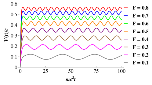
Figure 4: Velocity as a function of time for various forces listed in the legend ($F$ in units of $F_{\mathrm{max}}=2nmc^{2}$). Here $\kappa=20$, $G/c=20$ and $M=40m$. The dashed lines correspond to the drift velocity plotted in Fig. 5. One notices that as $F$ increases, the drift velocity and frequency of oscillations increases, while the velocity amplitude (as measured from $V_{\mathrm{D}}$) decreases.

Turning to the period of oscillations, Eq. (53) we use the relations $V\approx V_{\mathrm{D}}=\kappa F/2n^{2}$, $\dot{\Phi}\approx F/n$ to obtain the renormalized period of Bloch oscillations,

$$\tau_{\mathrm{B}}\approx\frac{2\pi n}{F}\left[1+\left(\frac{F}{2nmc^{2}}\right)^{2}\right].$$ (60)

The characteristic force entering Eq. (60) coincides with the upper bound $F_{\mathrm{max}}=2nmc^{2}$ obtained from Eq. (58) using the result (59) for the mobility. Indeed, the frequency of the motion $\omega\approx F/n$ should be small compared to the typical phonon frequency $mc^{2}$ in order to justify the large scale separation employed in Sec. II.

To go beyond lowest order in $F$ we devise a numerical approach to the strongly coupled impurity based on the Josephson form, Eq. (24) for the energy. Using it in Eq. (48) and recalling Eq. (47) gives,

$$\dot{P}=F-\frac{1}{2}\frac{\kappa V}{c^{2}-V^{2}}\dot{\Phi}^{2};\,\,\,\,\,\,\quad\quad\frac{\kappa\dot{\Phi}}{2n}=V-V_{c}\,\textrm{sin}\Phi,$$ (61)

where $P$ is given by Eq. (9). The second of Eqs. (61) relates the change in $\Phi$ with the deviation of the impurity velocity $V$ from its equilibrium value $V_{c}\sin\Phi$. The velocity $V(t)$ is obtained by solving Eqs. (61) numerically and the results depicted in Figs. 4 agree well with the ansatz (62). As one can see the precise choice of initial conditions is essentially irrelevant to the ensuing discussion, where we focus only on the asymptotic, steady state behavior of the functions $\Phi(t)$ and $V(t)$.

After a sufficiently long time the system reaches the regime of steady Bloch oscillations, where its velocity is given by

$$V(t)=V_{\mathrm{D}}+V_{\mathrm{B}}\cos(\omega_{\mathrm{B}}t+\delta)\,.$$ (62)

Here the parameters $V_{\mathrm{D}}$, $V_{\mathrm{B}}$, $\omega_{\mathrm{B}}=2\pi/\tau_{\mathrm{B}}$ and $\delta$ depend on the ratio of the external force $F$ to the critical force $F_{\mathrm{max}}$.

To find the drift velocity and period of Bloch oscillations we substitute the ansatz $V=V_{\mathrm{D}}$ and $\dot{P}=n\dot{\Phi}=\omega_{\mathrm{B}}$ into Eqs. (61) to obtain a closed set of equation,

$$n\omega_{\mathrm{B}}=F-\frac{1}{2}\frac{\kappa V_{\mathrm{D}}\omega_{\mathrm{B}}^{2}}{c^{2}-V_{\mathrm{D}}^{2}};\qquad\frac{\omega_{\mathrm{B}}}{2mc^{2}}=V_{\mathrm{D}}/c$$ (63)

which are solved to give

$$\frac{V_{\mathrm{D}}}{c}=\frac{\omega_{\mathrm{B}}}{2mc^{2}}=\frac{F_{\mathrm{max}}}{2F}\left(\sqrt{1+\left(\frac{2F}{F_{\mathrm{max}}}\right)^{2}}-1\right)\,.$$ (64)

Expanding the expression for $\omega_{\mathrm{B}}=2\pi/\tau_{\mathrm{B}}$ for small $F/F_{\mathrm{max}}$ one recovers the result (60) obtained by a different method. The results for the drift velocity are plotted in Fig. 5a and are in excellent agreement with numerical solution of Eqs. (61).

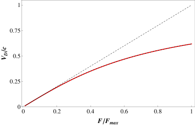
Figure 5: Drift velocity $V_{\mathrm{D}}$ (left panel) and amplitude $V_{\mathrm{B}}$ (right panel) as functions of the applied force $F$ corresponding to the same set of parameters are as in Fig. 4. The solid curve on left panel is indistinguishable from the analytic prediction, the first of Eqs. (64), while the dashed curve is the small force result Eq. (56) with mobility $\sigma=\kappa/2\hbar n^{2}$. On right panel the solid curve is numerics, the dashed curve is Eq. (126), and the dotted curve corresponds to the small F limit of Eq. (65).

The Bloch amplitude $V_{\mathrm{B}}$ can also be estimated from Eqs. (61). In Appendix D it is shown that

$$\qquad V_{\mathrm{B}}=V_{\mathrm{c}}\left\{1-\left[1+\frac{1}{2}\left(\frac{M-mN}{m\kappa}\right)^{2}\right]\left(\frac{F}{F_{\mathrm{max}}}\right)^{2}\right\}\,.$$ (65)

Thus, Eq. (65) predicts a decrease of the Bloch amplitude $V_{\mathrm{B}}$ with increasing $F$ (see Fig. 5b). Physically sensible, this result implies that as the force increases, the ideal equilibrium tracing of the dispersion relation is, to a degree, lost. This is due to the phononic subsystem gaining a proportionately larger share of the work done by the external force. Expression (65) is compared with results of the numerical solution of Eqs. (61) and the results presented in the right panel of Fig. 5b show a good agreement.

V.1.2 Weakly interacting background bosons and weak coupling regime $G/c\ll 1$

We deal with the case of the background made of weakly interacting bosons by using the Gross-Pitaevskii equation for the background Bose liquid as explained in Appendix C. By calculating numerically the dispersion relation of the impurity, see e.g. Fig. 1, we obtain the functions $N_{0}$ and $\Phi_{0}$ for all values of the impurity-background coupling $G$. The results of numerical evaluation of Eq. (57) are shown in Fig. 6.

Let us turn now to the case of weak coupling $G\ll c$, where particles can tunnel through the semi-transparent impurity. In such a case one expects the mobility to increase as the impurity becomes more transparent. For weak coupling, the main contribution to the integral in Eq. (57) comes from the region where the velocity of the impurity is maximal, i.e. $V\sim V_{\mathrm{c}}$. It corresponds to the inflection points of the dispersion, Fig. 1. Beyond this point the dispersion follows closely the dispersion of grey solitons, Eq. (97) and one can use the expressions (98) to estimate the mobility. As the momentum $P_{\mathrm{c}}$ corresponding to maximum velocity $V(P_{\mathrm{c}})=V_{\mathrm{c}}$ is small we simplify Eqs. (97), (98) and write

$$\frac{V(\Phi)}{c}\simeq 1-\frac{1}{2}\left(\frac{\Phi}{2}\right)^{2};\qquad\frac{P(\Phi)}{n}=\Phi-\sin\Phi\simeq\frac{\Phi^{3}}{6}\,$$ (66)

or, equivalently,

$$\Phi(P)=(6P/n)^{1/3};\qquad\frac{V(P)}{c}=1-\frac{(6P/n)^{2/3}}{8}\,.$$ (67)

Substituting these expressions into Eq. (57) we can estimate the mobility as

$$\sigma\sim\frac{\kappa}{n}\int_{P_{\mathrm{c}}}\frac{dP}{1-V^{2}/c^{2}}\left(\frac{\partial\Phi}{\partial P}\right)^{2}\sim\frac{\kappa}{n^{2}}\int_{\Lambda}\frac{dP/n}{(P/n)^{2}}\sim\frac{\kappa}{n^{2}}\frac{c}{G}=1/nmG\,.$$ (68)

Here we have estimated the momentum cutoff $\Lambda=P_{\mathrm{c}}/n\sim G/c$ using Eq. (114) for the critical velocity and the second equation in (67). The coefficient in Eq. (68) is fixed from the numerics and was found to be very close to one for $M=m$. Interestingly, in the weak coupling limit $\sigma$ is independent of the correlations within the liquid (provided the liquid is weakly interacting, $G\ll c$), diverging in the limit of a completely transparent impurity. Thus, in the weak coupling limit, the upper critical force $F_{\mathrm{max}}=nGmc$ corresponds to energy difference $Gn$ per healing length $\xi=1/mc$.

Figure 6: Log-log plot of the zero temperature mobility $\sigma$ as a function of the impurity coupling $G$ in a weakly interacting superfluid (solid line). The dashed lines correspond to the asymptotic values of $\sigma$ in the strong and weak coupling limits given by Eqs. (59) and (68), respectively (with $\hbar=1$). The Luttinger parameter for the liquid is taken to be $\kappa=n/mc=20$, while $M=m$.

VI Finite temperature dynamics of depleton. Backscattering of thermal phonons and viscous friction

At a finite temperature, even in the absence of the external force, the collective coordinates fluctuate around their equilibrium position $\Lambda_{\pm}^{(0)}$, found from the condition $\partial_{\Lambda}H=0$. Assuming these fluctuations are small, one may linearize Eq. (46) near its equilibrium point. Being transformed to the frequency representation, such linearized matrix equation of motion takes the form

$$\left(-\frac{i\omega}{2}+\mathsf{\Gamma}^{-1}\right)\Lambda(\omega) = \xi(\omega)\,,$$ (69)

where $\mathsf{\Gamma}$ is the Hessian matrix of the second derivatives of the impurity Hamiltonian at fixed momentum $P$. Its matrix elements are

$$\mathsf{\Gamma}^{-1}=\begin{pmatrix}\Gamma_{++}&\Gamma_{+-}\\ \Gamma_{-+}&\Gamma_{--}\end{pmatrix}^{-1}=\left.\begin{pmatrix}H_{\Lambda_{+}\Lambda_{+}}&H_{\Lambda_{+}\Lambda_{-}}\\ H_{\Lambda_{-}\Lambda_{+}}&H_{\Lambda_{-}\Lambda_{-}}\end{pmatrix}\right|_{\Lambda=\Lambda^{(0)}}$$ (70)

Solution of equation (69) takes the form

$$\Lambda(\omega)=\left(1-\frac{i\omega}{2}\mathsf{\Gamma}\right)^{-1}\,\mathsf{\Gamma}\,\xi(\omega)=\mathsf{\Gamma}\,\xi(\omega)+\frac{i\omega}{2}\mathsf{\Gamma}^{2}\,\xi(\omega)+\ldots\,,$$ (71)

where we consider it as a perturbative sequence in frequency, to avoid spurious instabilities mentioned in Section V. Substituting this solution into the right hand side of Eq. (45) and averaging it over the Gaussian noise (43), one finds for the momentum loss rate

$$\dot{P}=F_{\mathrm{fr}}=-\frac{1}{2}\int\frac{d\omega}{2\pi}\,\,\omega^{2}\,\mbox{Tr}\Big{\{}\big{\langle}\xi(\omega)\xi^{\dagger}(\omega)\big{\rangle}\big{(}\mathsf{\Gamma}^{\dagger}\mathsf{V}^{-1}\mathsf{\Gamma}-\mathsf{V}^{-1}\mathsf{\Gamma}^{\dagger}\mathsf{\Gamma}\big{)}\Big{\}}=-\frac{1}{2}\int\frac{d\omega}{2\pi}\,\,\omega^{3}\,\mbox{Tr}\Big{\{}\mathsf{F}(\omega)\big{[}\mathsf{\Gamma}^{\dagger},\mathsf{V}^{-1}\big{]}\mathsf{\Gamma}\Big{\}}\,,$$ (72)

where we kept only leading order in frequency. The matrix-valued function $\mathsf{F}(\omega)$ is odd in frequency, selecting only odd powers of $\omega$ from the expression it is multiplied by. Equation (72) provides the expression for the viscous friction force acting on the impurity from the normal component of the liquid. It can be identified with the Raman two-phonon scattering mechanism Gangardt09 ; Gangardt2010Quantum ; Muryshev2002Dynamics ; LandauKhalatnikov1949ViscosityI ; LandauKhalatnikov1949ViscosityII .

Substituting the explicit form of the Ohmic noise correlator (41) and performing the frequency integration, one finds for the friction force

$$F_{\mathrm{fr}}=-\big{|}{\Gamma}_{+-}\big{|}^{2}\frac{c\,}{c^{2}-V^{2}}\int\!\frac{d\omega}{2\pi}\,\,\omega^{3}\left(\coth\frac{\omega}{2T_{-}}-\coth\frac{\omega}{2T_{+}}\right)=-\frac{16\pi^{3}}{15}\big{|}{\Gamma}_{+-}\big{|}^{2}\frac{T^{4}}{c^{2}}\left(\frac{c^{2}+V^{2}}{c^{2}-V^{2}}\right)V\,.$$ (73)

The $T^{4}$ dependence of the friction force was reported in castro96 and is a direct consequence of the phase space for two-phonon scattering. It can be also viewed as a one-dimensional version of the Khalatnikov-Landau result LandauKhalatnikov1949ViscosityI ; LandauKhalatnikov1949ViscosityII for the viscosity of liquid helium. It should be noted that the friction force (73) is proportional to the off-diagonal matrix element $\Gamma_{+-}$ which represents backscattering of phonons by the depleton. It depends on the momentum $P$ and, consequently velocity $V$ of the mobile impurity in addition to the parameters of the impurity-background interactions. Below we derive the general expression for the backscattering amplitude and relate it to the equilibrium dispersion $E(P,n)$ of the depleton.

VI.1 Backscattering amplitude

The detailed information about microscopic impurity-liquid interactions is contained in the off-diagonal matrix element $\Gamma_{+-}$ which represents the effective vertex for two-phonon scattering. In the spirit of our phenomenological approach it may be expressed, as explained in Appendix E, through partial derivatives of the equilibrium values $\Phi_{0}(V,n)$ and $N_{0}(V,n)$,

$${\Gamma}_{+-}(V,n) = -\frac{\kappa m}{M^{*}}\left[\frac{M-mN}{mn}\left(\frac{\partial\Phi_{0}}{\partial V}+m\frac{\partial N_{0}}{\partial n}\right)+\left(\frac{\partial\Phi_{0}}{\partial V}\frac{\partial N_{0}}{\partial n}-\frac{\partial\Phi_{0}}{\partial n}\frac{\partial N_{0}}{\partial V}\right)\right].$$ (74)

Treating collective variables $\Phi_{0}=\Phi_{0}(P,n)$ and $N_{0}=N_{0}(P,n)$ as function of momentum rather than velocity and calculating the corresponding derivatives as explained in Appendix E we find an alternative representation

$${\Gamma}_{+-}(P,n) = -\frac{1}{c}\left(\frac{M}{m}\frac{\partial\Phi_{0}}{\partial P}+\Phi_{0}\frac{\partial N_{0}}{\partial P}-N_{0}\frac{\partial\Phi_{0}}{\partial P}+\frac{\partial N_{0}}{\partial n}\right).$$ (75)

The functions $\Phi_{0}$ and $N_{0}$ are obtained from the equilibrium dispersion $E(P,n)$ as explained in Section III.2 (see, e.g. Eq. (21)). This relations can be used to obtain an equivalent representation for the backscattering amplitude ${\Gamma}_{+-}$ given by Eq. (137) in Appendix E.

Figure 7: $V=0$ and $\Phi=0$ (i.e., $P=0$) dissipation rate as a function of the impurity coupling $G$ for $\kappa=10$ and $M=m$ (solid line). The dashed line corresponds to the strong coupling $G\gg c$ limit, Eq. (76).

Two remarks are in order. First, it should be noticed that the backscattering amplitude given by Eqs. (74), (75) depends on the velocity $V$ or momentum $P$ of the depleton. While the momentum dependence is unambiguous, there can be different regimes corresponding to the same velocity characterized by different values of the superfluid phase $\Phi$. Second, it can be shown by calculating dispersion $E(P,n)$ by Bethe Ansatz method that the off-diagonal matrix element $\Gamma_{+-}$ vanishes identically for integrable mobile impurities, such as lowest excitation branch in Lieb-Liniger Lieb_Liniger_1963 or Yang-Gaudin CN_Yang_1967 ; Gaudin_1967 models and the soliton of the Gross-Pitaevskii equation (see Appendix B). We postpone the details of these exact calculations to another publication. Below we use the semiclassical approach valid for the weakly interacting bosonic background which provides results for backscattering amplitude in a wide range of parameters relevant to experiments.

VI.1.1 Strong coupling regime $G/c\gg 1$

In the strong coupling regime the leading terms in the the number of depleted particles, the second equation in (116) is a constant, $N_{0}=2\kappa\gg 1$ and the momentum is dominated by the supercurrent and $P=n\Phi$. These observation simplify greatly the expression (75) for backscattering amplitude and one gets

$$\Gamma_{+-}=\frac{1}{mc^{2}}\left[1-\frac{M}{\kappa m}\right]\,,$$ (76)

where we have used the fact that $\partial\kappa/\partial n=\kappa/2n$. The expression (76) is momentum or velocity independent constant, which equals $1/mc^{2}$ for a not too heavy impurity $M\ll\kappa m$.

VI.1.2 Weak coupling regime $G/c\ll 1$ for slow impurity

In the weak coupling regime the backscattering amplitude varies strongly with the velocity of the depleton. Here we present results for slow impurity which can be found by evaluating $\Gamma_{+-}$ for $V=0$.

There are two distinct physical regimes corresponding to a slow impurity: one, corresponding to the solution with $\Phi_{0}\simeq 0$ and momentum $P\simeq MV\simeq 0$ dominated by the bare impurity and one corresponding to $\Phi_{0}\simeq\pi$ and momentum $P\simeq\pi n$ dominated by the background supercurrent. For $\Phi\approx 0$ we have

$$N_{0}(V,n)=2\kappa\left(1+\frac{G}{2c}-\sqrt{1+\left(\frac{G}{2c}\right)^{2}}\right)\,,\qquad\Phi_{0}(V,n)=2\frac{V}{c}\left(-1+\frac{G}{2c}+\sqrt{1+\left(\frac{G}{2c}\right)^{2}}\right),$$ (77)

while near $\Phi=\pi$, we find

$$N_{0}(V,n)=2\kappa\,,\qquad\Phi_{0}(V,n)=\pi-2\frac{V}{c}\left(1+\frac{G}{c}\right)\,.$$ (78)

These expressions are correct up to terms $\mathcal{O}(V^{2})$ for the number of particles and $\mathcal{O}(V^{3})$ for the phase.

In the case $\Phi_{0}\simeq 0$ we use Eqs. (77) to calculate $\Gamma_{+-}$. For weak coupling to the leading order in both $g/c=1/\kappa$ and $G/c$ we have,

$$\Gamma_{+-}=\frac{1}{mc^{2}}\left(\frac{G}{c}\right)\left(\frac{mG}{Mg}-1\right)\,,\qquad G/c\ll 1.$$ (79)

This result agrees with Eq.(5) in Ref. Gangardt09 and indicates that friction vanishes near integrable point $M=m$ and $G=g$, at least for small velocities near $\Phi=0$. The results for arbitrary coupling $G/c$ are presented in Figs. 7.

In the case $\Phi_{0}\simeq\pi$, we use Eqs.(78) and calculate effective mass $M^{*}=M-mN+n\partial_{V}\Phi=M-2\kappa m-2\kappa m(1+G/c)$. Using Eq.(74) we find for arbitrary coupling

$$\Gamma_{+-}=\frac{1}{mc^{2}}\frac{(M/\kappa m)\left(1+2G/c\right)-2G/c}{M/\kappa m-2G/c-4},$$ (80)

It comes as no surprise that Eq.(80) vanishes in the limit $M,G\rightarrow 0$, where one recovers the dark soliton result from Appendix B. Indeed, there it is mentioned that such soliton excitation is transparent for phonons due to its integrability and, consequently, $\Gamma_{+-}=0$ for all velocities. In the limit of weak coupling Eq.(80) becomes

$$\Gamma_{+-}=\frac{1}{mc^{2}}\left(\frac{2G}{c}-\frac{M}{\kappa m}\right)\,.$$ (81)

At the Yang-Gaudin integrable point (CN_Yang_1967 ; Gaudin_1967 , see also zvonarev_2007 ) of the quantum system defined as $M=m$ and $G=g$, the corresponding limit of the second equation in (81) is proportional $g/c=1/\kappa$ which is a small parameter in the semiclassical limit and therefore our calculation goes beyond the accuracy of the approximations adopted above.

VI.2 Bloch oscillations in the presence of viscous friction

Imagine the impurity is dragged by the weak external force $F$. There is a velocity $V<V_{\mathrm{c}}$ such that $F+F_{\mathrm{fr}}(V)=0$ and the system reaches a steady state with constant drift velocity $V_{\mathrm{D}}$ and no oscillations, $V_{\mathrm{B}}=0$. If the applied force is very small, the drift velocity can be found from the small velocity limit of Eq. (73) in the linear response form, $V_{\mathrm{D}}=\sigma_{T}F$, where the finite temperature mobility is given by

$$\sigma^{-1}_{T}=\frac{16\pi^{3}}{15}\frac{T^{4}}{c^{2}}\big{|}\Gamma_{+-}(V=0)\big{|}^{2}.$$ (82)

in accordance with castro96 ; Gangardt09 . Increasing the external force, leads to a slightly nonlinear dependence of the drift velocity on $F$ (due to the non-linear velocity dependence of $F_{\textrm{fr}}(V)$, cf. Eq. (73)), until the the maximal possible velocity $V_{\mathrm{c}}$ is reached for $F=F_{\mathrm{min}}=-F_{\mathrm{fr}}(V_{c})$. Beyond this critical force no steady state solution can be found and the impurity performs Bloch oscillations along with the drift. In such a nonlinear regime the amplitude, period of the oscillations, drift velocity, as well as the momentum-dependent viscous backscattering amplitude, Eq. (75), are controlled by the equilibrium dispersion relation.

We illustrate the above scenario using the model of a strongly coupled impurity. In this case the critical velocity is small and backscattering amplitude is velocity-independent. The critical force is then found from the linear response as $F_{\mathrm{min}}=V_{\mathrm{c}}/\sigma_{T}$. We can use the relation $V=V_{\mathrm{c}}\sin\Phi+\kappa\dot{\Phi}/2n$ (i.e., the second of Eqs. (61)) and the fact that $P=n\Phi$ to write down the equation of motion for the superfluid phase,

$$\dot{\Phi}=\frac{F_{\mathrm{min}}}{n(1+\kappa/2\sigma_{T}n^{2})}\Big{(}\lambda-\sin\Phi\Big{)}\,,$$ (83)

where $\lambda=F/F_{\mathrm{min}}$. Introducing dimensionless time variable $s=(F_{\mathrm{min}}/n(1+\kappa/2\sigma_{T}n^{2}))t$ and assuming, without loss of generality, $\Phi(0)=0$, the solution of Eq. (83) is found to be

$$\tan\frac{\Phi}{2}=\frac{\lambda\tanh\left(\frac{\sqrt{1-\lambda^{2}}}{2}s\right)}{\sqrt{1-\lambda^{2}}+\tanh\left(\frac{\sqrt{1-\lambda^{2}}}{2}s\right)}$$ (84)

For $\lambda<1$ it describes velocity approaching its limiting value $V_{\infty}=V_{\mathrm{c}}\sin\Phi(\infty)=\lambda V_{\mathrm{c}}$. For $\lambda>1$ Eq. (84) describes a periodic function with period

$$\tau_{\mathrm{B}}=\frac{t}{s}\frac{2\pi}{\sqrt{\lambda^{2}-1}}=\frac{2\pi n(1+\kappa/2\sigma_{T}n^{2})}{\sqrt{F^{2}-F^{2}_{\mathrm{min}}}}\,.$$ (85)

The corresponding drift velocity for $F>F_{\textrm{min}}$ can be found by averaging the momentum relation $n\dot{\Phi}=F-V/\sigma_{T}$ over a single period with the result

$$V_{\mathrm{D}}=V_{c}\left(\frac{F}{F_{\mathrm{min}}}-\frac{\sqrt{F^{2}/F_{\mathrm{min}}^{2}-1}}{1+\kappa/2\sigma_{T}n^{2}}\right).$$ (86)

For $F_{\mathrm{min}}\ll F\ll F_{\mathrm{max}}$, one may expand Eq. (86) to obtain a small temperature correction

$$V_{\mathrm{D}}/c\approx\frac{F}{F_{\mathrm{max}}}+\frac{c}{V_{c}}\frac{F_{\mathrm{min}}}{F}\left(\frac{1}{2}V_{c}^{2}/c^{2}-(F/F_{\mathrm{max}})^{2}\right),$$ (87)

which gives the previous result Eq. (59) in the limit of small $T$, or more specifically, small $F_{\mathrm{min}}$. Interestingly, Eq. (87) predicts an increase in the drift with increasing $T$ if $F/F_{\mathrm{max}}\lesssim V_{c}/c$. This suggests that for a small enough force, a significant drop in the drift velocity may occur as the system is cooled below the critical temperature, when the impurity enters the regime of Bloch oscillations, see Fig. 8.

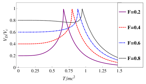
Figure 8: Drift velocity of a strongly coupled impurity in a weakly interacting bose liquid as a function of temperature $T$ for various forces as predicted by Eq. (86). $F$ is given in units of $F_{\mathrm{max}}V_{c}/c$, while the Luttinger parameter is taken to be $K=\pi\kappa=8\pi^{4}/15\approx 52$ so that, to a good approximation, $F_{\mathrm{min}}(T=mc^{2})=F_{\mathrm{max}}V_{c}/c$.

The above analysis demonstrates, inter alia, a non-monotonic dependence of the drift velocity on the parameter $F/F_{\mathrm{min}}$ as it is increases past 1 and enters the regime of Bloch oscillations. This may occur either by fixing the temperature and increasing the force, or by fixing the external force and cooling the system. In contrast to the vanishing amplitude $V_{\mathrm{B}}$ near $F_{\mathrm{max}}$, indicated by the second equation in (64), it is rather the divergent period, Eq. (85) for $F$ approaching $F_{\mathrm{min}}$ from above which leads to the disappearance of Bloch oscillations.

VII Discussion of the results

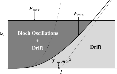
Figure 9: Schematic force vs. temperature diagram of impurity motion in a 1D quantum liquid. In the region $F<F_{\textrm{min}}$ (light gray) the impurity drifts with mobility $\sigma_{T}\propto T^{-4}$ for $T\ll mc^{2}$. For $T\gg mc^{2}$, the mobility scales $\sigma_{T}\propto T^{-1}$ (dashed are the small and large temperature asymptotics). For $F_{\textrm{min}}<F<F_{\textrm{max}}$ (dark gray) one has Bloch oscillations + drift. Above $F_{\textrm{max}}$, our theory is inapplicable and we expect some kind of incoherent acceleration, possibly corresponding to a supersonic impurity which has escaped its self-induced depletion cloud.

The coupling with phonons governed by the universal term, Eq. (29), results in transfer of energy and momentum between the depleton and the background. At zero temperature it takes the form of radiation of phonons by accelerated impurity similar to the radiative damping in classical electrodynamics Ginzburg_Applications_of_Electrodynamics and leads to the finite mobility of the depleton. For sufficiently weak forces the mobility, defined as the ratio of the drift velocity to the applied force, see Eq. (56) can be expressed via equilibrium dispersion, Eq. (57) reminiscent of the Kubo linear response theory. The drift, however, is superimposed with the essentially non-linear Bloch oscillations of the velocity. The amplitude of the oscillations is shown to vanish as the external force attains the upper critical force $F_{\mathrm{max}}$ reflecting the limit of validity for the description based on the scale separation between the healing length and the phonon wavelength.

At finite temperature the thermal phonons present in the system are scattered by the depleton leading to the viscous friction force, Eq. (73). This in turn leads to the appearance of the lower critical force $F_{\mathrm{min}}(T)\sim T^{4}$ which sets the lower limit for the external force driving the Bloch oscillation. In contrast to the situation in the vicinity of $F_{\mathrm{max}}$, the approach to $F_{\mathrm{min}}$ makes the Bloch oscillation disappear through the divergence of the period, Eq. (85). Below $F_{\mathrm{min}}$ the system enters the regime of non-oscillatory drift characterized by the velocity $V_{\mathrm{D}}<V_{\mathrm{c}}$, where all the momentum provided by the external force is dissipated into phononic bath.

The viscous force contains valuable information about the fine details of the interactions between particles. In this work we have confirmed and extended the earlier observation Gangardt09 , that the backscattering amplitude, given in terms of equilibrium properties by Eqs. (74), (75) vanishes if the depleton is an elementary excitation of an integrable model. This includes the dark soliton excitation of Lieb-Liniger model Lieb_Liniger_1963 as well as spinons in bosonic Yang-Gaudin model CN_Yang_1967 ; Gaudin_1967 . The microscopic mechanism responsible for the absence of dissipation is due to destructive quantum interference between various two-phonon processes. It can be traced back to the absence of three-body processes lying at heart of integrability in one dimension. In contrast, the radiative processes due to the presence of external force are always present in the dynamics of the depleton. This is because the external potential is not, in general, compatible with the integrability.

Various dynamical regimes of depleton are summarized in diagram Fig. 9. At sufficiently low temperatures there is a wide parametric window $F_{\mathrm{min}}<F<F_{\mathrm{max}}$ for the external force in which the Bloch oscillations can be observed experimentally. At temperatures higher than chemical potential the mobility of the particle becomes inversely proportional to temperature Muryshev2002Dynamics ; Gangardt2010Quantum and moderates the growth of $F_{\mathrm{min}}$ (see Fig. 9). The above range of forces can be increased further by exploring the dependence of $F_{\mathrm{min}}$ and $F_{\mathrm{max}}$ on the interaction parameters. In particular, at integrable point $F_{\mathrm{min}}$ vanishes for any temperature.

Our approach to the dynamics of depleton is essentially classical, the quantum mechanics enters only via parameters of the effective action. The equations of motion, Eqs. (46) neglect therefore the quantum and thermal fluctuations of the collective variables of the depleton. These fluctuations can be taken into account by either simulating the Langevin equation in the presence of equilibrium noises or by writing appropriate Fokker-Planck equation for the distribution function. One of the most important consequence of the fluctuations is expected to be the smearing the boundaries between dynamical regimes in Fig. 9. We leave this as well as the question about the role of quantum fluctuation for further investigation. Another important extension of the present work would be the studies of the finite size effects due to the trap geometry relevant for experiments with ultracold atoms.

VIII Acknowledgments

We are indebted to L. Glazman, A. Lamacraft, M. Zvonarev, I. Lerner and J.M.F. Gunn for illuminating discussions. MS and AK were supported by DOE contract DE-FG02-08ER46482. DMG acknowledges support by EPSRC Advanced Fellowship EP/D072514/1. DMG and AK are thankful to Abdus Salam ICTP in Trieste for hospitality at the early stages of this work.

Appendix A Derivation of dissipative action

Gaussian integration of the interaction term Eq. (38) using the following phononic propagators

$$-i\Big{\langle}\chi^{\phantom{\dagger}}_{\mathrm{cl}}(x,t)\chi^{\dagger}_{\mathrm{cl}}(x^{\prime},t^{\prime})\Big{\rangle} = \mathsf{D}^{K}(x-x^{\prime},t-t^{\prime}),\qquad-i\Big{\langle}\chi^{\phantom{\dagger}}_{\mathrm{q}}(x,t)\chi^{\dagger}_{\mathrm{cl}}(x^{\prime},t^{\prime})\Big{\rangle}=\mathsf{D}^{A}(x-x^{\prime},t-t^{\prime})$$

$$-i\Big{\langle}\chi^{\phantom{\dagger}}_{\mathrm{cl}}(x,t)\chi^{\dagger}_{\mathrm{q}}(x^{\prime},t^{\prime})\Big{\rangle} = \mathsf{D}^{R}(x-x^{\prime},t-t^{\prime}),\qquad-i\Big{\langle}\chi^{\phantom{\dagger}}_{\mathrm{q}}(x,t)\chi^{\dagger}_{\mathrm{q}}(x^{\prime},t^{\prime})\Big{\rangle}=0$$ (88)

leads to the quadratic nonlocal action

$$S_{\mathrm{eff}} = \frac{1}{2}\int\!\mathrm{d}t\mathrm{d}t^{\prime}\;\dot{\Lambda}^{\dagger}_{\mathrm{cl}}(t)\;\partial_{t}\Big{[}\mathsf{\Delta}^{R}(t-t^{\prime})-\mathsf{\Delta}^{A}(t-t^{\prime})\Big{]}\left[\Lambda_{\mathrm{q}}(t^{\prime})+\mathsf{V}^{-1}\dot{\Lambda}_{\mathrm{cl}}(t^{\prime})X_{\mathrm{q}}(t^{\prime})\right]$$ (89)

$$- \frac{1}{2}\int\!\mathrm{d}t\mathrm{d}t^{\prime}\,\left[\Lambda^{\dagger}_{\mathrm{q}}(t)+X^{\phantom{\dagger}}_{\mathrm{q}}(t)\dot{\Lambda}^{\dagger}_{\mathrm{cl}}(t)\mathsf{V}^{-1}\right]\partial^{2}_{t}\mathsf{\Delta}^{K}(t-t^{\prime})\left[\Lambda_{\mathrm{q}}(t^{\prime})+\mathsf{V}^{-1}\dot{\Lambda}_{\mathrm{cl}}(t^{\prime})X_{\mathrm{q}}(t^{\prime})\right]\,,$$

where $\mathsf{\Delta}^{R,A,K}(t)=\mathsf{D}^{R,A,K}(Vt,t)$ are phonon propagators restricted to the impurity trajectory.

Inverting the matrix in Eq. (33) and taking appropriate analytic structure in the complex $\omega$ plane we obtain Fourier components of the retarded and advanced propagators,

$$\mathsf{D}^{R}(q,\omega)=\Big{[}\mathsf{D}^{A}(q,\omega)\Big{]}^{\dagger}=\int\!dxdt\;e^{-iqx+i\omega t}\,\mathsf{D}^{R}(x,t)=\begin{pmatrix}\frac{1}{q(\omega-cq+i0)}&0\\ 0&-\frac{1}{q(\omega+cq+i0)}\end{pmatrix}\,.$$ (90)

This leads to

$$\mathsf{D}^{R}(q,\omega)-\mathsf{D}^{A}(q,\omega)=\frac{2\pi}{iq}\begin{pmatrix}\delta(\omega-cq)&0\\ 0&-\delta(\omega+cq)\end{pmatrix}$$ (91)

and, subsequently,

$$\partial_{t}\Big{[}\mathsf{\Delta}^{R}(t)-\mathsf{\Delta}^{A}(t)\Big{]}=\frac{1}{2\pi}\int\mathrm{d}q\,\mathrm{d}\omega\,e^{i(qV-\omega)t}\left(\frac{qV-\omega}{q}\right)\begin{pmatrix}\delta(\omega-cq)&0\\ 0&-\delta(\omega+cq)\end{pmatrix}=-\begin{pmatrix}\delta(t)&0\\ 0&\delta(t)\end{pmatrix}$$ (92)

The noise terms, i.e. the second line of Eq. (89) are controlled by the Keldysh component $D^{K}$ and its derivatives. Assuming thermal equilibrium of phonons in the laboratory frame and using Fluctuation-Dissipation Theorem we have

$$\mathsf{D}^{K}(q,\omega) = \coth\left(\frac{\omega}{2T}\right)\Big{(}\mathsf{D}^{R}(q,\omega)-\mathsf{D}^{A}(q,\omega)\Big{)}\,.$$ (93)

Using Eq. (91) we find the Fourier component of the Keldysh propagator restricted to the classical trajectory

$$\Delta^{K}(\omega) = \int\frac{\mathrm{d}q}{2\pi}\,\coth\left(\frac{\omega+qV}{2T}\right)\Big{(}\mathsf{D}^{R}(q,\omega+qV)-\mathsf{D}^{A}(q,\omega+qV)\Big{)}=\frac{1}{i\omega}\begin{pmatrix}\coth\frac{\omega}{2T}\frac{c}{c-V}&0\\ 0&\coth\frac{\omega}{2T}\frac{c}{c+V}\end{pmatrix},$$

Substituting its Fourier transform it into Eq. (89) and taking double time derivative leads to the second term in Eq. (40).

Appendix B Grey Solitons

Dynamic properties of one-dimensional bosons of mass $m$ weakly interacting via repulsive short range potential proportional to coupling constant $g$ can be studied within the Gross-Pitaevskii description using the following Lagrangian

$$L=\int\mathrm{d}x\left(i\bar{\psi}\partial_{t}\psi-\frac{1}{2m}\left|\partial_{x}\psi\right|^{2}-\frac{g}{2}\left|\psi\right|^{4}+\mu\left|\psi\right|^{2}\right)\,.$$ (94)

Here $\psi$ is the quasi-condensate wavefunction corresponding to the asymptotic density $|\psi(\pm\infty,t)|^{2}=n$ and vanishing supercurrent at infinity. The condition of weak interactions is $mg/n\ll 1$. Minimizing the action defined by the Lagrangian Eq. (94) leads to the Gross-Pitaevskii equation,

$$i\partial_{t}\psi=\left(-\frac{\partial_{x}^{2}}{2m}+g|\psi|^{2}-\mu\right)\psi.$$ (95)

Substituting a constant solution $\psi_{0}=\sqrt{n}$ one obtains the chemical potential $\mu=gn=mc^{2}$ related to the sound velocity $c=\sqrt{gn/m}$. In addition to uniform solution, Gross-Pitaevskii equation (108) admits a one-parameter family of solutions

$$\psi_{\mathrm{s}}(x-Vt;\Phi_{\mathrm{s}})=\sqrt{n}\left(\textrm{cos}\left(\frac{\Phi_{\mathrm{s}}}{2}\right)-i\textrm{sin}\left(\frac{\Phi_{\mathrm{s}}}{2}\right)\textrm{tanh}\left(\frac{x-Vt}{l}\right)\right),$$ (96)

known as grey solitons PitaevskiiStringariBook ; Tsuzuki_1971 . They can be visualized as a dip moving with velocity $V$ and having a core size $l=1/m\sqrt{(c^{2}-V^{2})}$. The solution, Eq. (96) is characterized by the total phase drop and number of expelled particles related to the velocity as

$$\Phi_{\mathrm{s}}(V,n) = 2\arccos\frac{V}{c},\qquad N_{\mathrm{s}}(V,n)=\int\mathrm{d}x\,\left(n-|\psi_{\mathrm{s}}(x)|^{2}\right)=\frac{2}{g}\sqrt{c^{2}-V^{2}}\,.$$ (97)

Momentum and energy of the soliton are given by Tsuzuki_1971 ; Shevchenko1988 ; Konotop2004Landau

$$P_{\mathrm{s}}=n\Phi_{\mathrm{s}}-mN_{\mathrm{s}}V\,,\qquad E_{\mathrm{s}}=\frac{4}{3}cn\sin^{3}(\Phi_{\mathrm{s}}/2)=\frac{mg^{2}}{6}N_{\mathrm{s}}^{3}$$ (98)

which allows to define the Lagrangian

$$L_{\mathrm{s}}(V,n)=(n\Phi_{\mathrm{s}}-mN_{\mathrm{s}}V)V-\frac{mg^{2}}{6}N_{\mathrm{s}}^{3},$$ (99)

Using soliton Lagrangian (99) and putting $M=0$ in Eqs. (17) and (18) one sees immediately that the variables in (97) coincide with the collective variables $\Phi$, $N$. Therefore the grey soliton can be viewed as a model for a massless impurity consisting of depletion cloud only.

We invert Eqs. (97) which yields

$$V_{0}=\frac{gN}{2\tan\frac{\Phi}{2}},\qquad n_{0}=\frac{mgN^{2}}{4\sin^{2}\frac{\Phi}{2}}\,.$$ (100)

Using Eq. (20) together with Eqs. (97) and (99) yields the internal energy, Eq. (23) of the soliton,

$$H_{\mathrm{d}}(N,\Phi) = \frac{mg^{2}}{6}N^{3}+N\left(\frac{mV_{0}^{2}}{2}-gn_{0}\right)=\frac{mg^{2}N^{3}}{8}\left(\frac{1}{3}-\frac{1}{\sin^{2}\Phi/2}\right).$$ (101)

The matrix of second derivatives at the equilibrium solution reads

$$\mathsf{H}=\begin{pmatrix}H_{\Phi\Phi}&H_{\Phi N}\\ H_{N\Phi}&H_{NN}\end{pmatrix}=\begin{pmatrix}-cn\frac{1+\cos^{2}\Phi/2}{\sin\Phi/2}&2mc^{2}\frac{\cos\Phi/2}{\sin\Phi/2}\\ 2mc^{2}\frac{\cos\Phi/2}{\sin\Phi/2}&-\frac{m^{2}c^{3}}{n}\frac{1+\cos^{2}\Phi/2}{\sin\Phi/2}\end{pmatrix}$$ (102)

The backscattering amplitude $\Gamma_{+-}$, calculated with the help of Eq. (127), vanishes identically due to the integrability Note1 of the Gross-Pitaevskii equation (95).

As it was shown in Fedichev1999Dissipative ; Muryshev2002Dynamics a weak cubic nonlinearity $-(\alpha/6)|\psi|^{6}$ in the Lagrangian (94) breaks the integrability of the model. Cubic terms describe three-body interactions which arise from virtual transitions to higher transverse states of tightly confined one-dimensional liquid Mazets2008Breakdown . Here we extent the results in Ref.Gangardt2010Quantum and calculate the amplitude of the corresponding dissipation processes for the whole range of soliton velocities.

The corresponding correction to the Lagrangian, Eq. (99) of the soliton can be calculated to the leading order by evaluating it with the unperturbed solution,

$$\delta L_{\mathrm{d}}=-\frac{\alpha}{6}\int\left(|\psi_{\mathrm{d}}(x)|^{2}-n\right)^{3}=\frac{8}{45}\frac{\alpha n^{3}}{mc}\left(1-\frac{V^{2}}{c^{2}}\right)^{5/2}=\frac{\alpha m^{2}g^{2}}{180}N^{5}=-\delta H_{\mathrm{d}}.$$ (103)

Here we have used the expression Eq. (97) for the number of expelled particles $N$ to calculate the correction to the energy relying on the theorem of small increments. The corresponding change in the matrix (102) of second derivatives

$$\mathsf{\delta H}=-\frac{\alpha m^{2}g^{2}}{9}N^{3}\times\begin{pmatrix}0&0\\ 0&1\end{pmatrix}$$ (104)

can be taken perturbatively in the calculation of the off-diagonal matrix element $\delta\Gamma_{+-}$. We have

$$\mathsf{\delta\Gamma}=-\mathsf{\Gamma}\left(\mathsf{T^{-1}\delta H\left({T^{-1}}\right)^{\dagger}}\right)\mathsf{\Gamma}\,.$$ (105)

Substituting Eqs. (104), (31), yields

$$\delta\Gamma_{+-}=\frac{\alpha\kappa m^{2}g^{2}}{18}N^{3}\,\Gamma_{++}\Gamma_{--}=\frac{\alpha\kappa m^{2}g^{2}}{18}\frac{N^{3}}{\det\mathsf{H}}$$ (106)

Here we have used the fact that the matrix $\mathsf{\Gamma}$ is diagonal in the leading order in $\alpha$ and $\det(\mathsf{T^{\dagger}T})=1$. The determinant of the matrix (102) is $\det\mathsf{H}=\left(mc^{2}\sin\Phi/2\right)^{2}$. Substituting it into Eq. (106) and using (97) leads to

$$\Gamma_{+-}=-\frac{4}{9}\frac{\alpha n^{2}}{m^{2}c^{4}}\left(1-\frac{V^{2}}{c^{2}}\right)^{1/2}$$ (107)

in agreement with the results of Ref.Gangardt2010Quantum .

Appendix C Impurity in a weakly interacting liquid

To model the impurity coupled to a weakly interacting superfluid at $T=0$, the Gross-Pitaevskii equation, Eq. (95) is modified in the presence of a delta function potential moving with constant velocity $V$

$$i\partial_{t}\psi=\left(-\frac{\partial_{x}^{2}}{2m}+g|\psi|^{2}-\mu+G\delta(x-Vt)\right)\psi.$$ (108)

Figure 10: Superfluid density in the presence of an impurity moving with velocity $V/c=0.6$ and coupling $G/c=0.1$ (solid line). The dashed lines corresponds to the double soliton solution Eq.(96) used to construct Eq.(109).

For $G>0$, the soliton solution, Eq. (96) still satisfies Eq.(108) except at the location of the impurity. Thus, one may construct a solution to Eq.(108) by matching two soliton solutions, Eq. (96) at the location of the impurity, as shown in Fig. 10. The proper solutions of Eq, (108) can thus be written

$$\psi(y)=\begin{cases}\psi_{\mathrm{s}}(y+x_{0};\Phi_{\mathrm{s}})e^{i\Phi_{0}/2},&y>0\\ \psi_{\mathrm{s}}(y-x_{0};\Phi_{\mathrm{s}})e^{-i\Phi_{0}/2},&y<0\end{cases}$$ (109)

where $y=x-Vt$ and velocity is always related as $V/c=\cos(\Phi_{\mathrm{s}}/2)$ to the phase $\Phi_{\mathrm{s}}$ parameterizing the soliton configuration, Eq. (96). The solutions $\psi_{\pm}$ to the right (left) of the impurity satisfy the boundary conditions: $\psi_{+}(0)=\psi_{-}(0),\,\psi_{+}^{\prime}(0)-\psi_{-}^{\prime}(0)=2mG\psi(0)$. Using (109), the boundary conditions give rise to the following two equations for $\Phi_{0}$ and $z=\textrm{tanh}(x_{0}/l)$

$$\tan\left(\frac{\Phi_{0}}{2}\right) = z\,\tan\left(\frac{\Phi_{s}}{2}\right)$$ (110)

$$\sin^{3}\left(\frac{\Phi_{\mathrm{s}}}{2}\right)\left(1-z^{2}\right)z = \frac{G}{c}\left[\cos^{2}\left(\frac{\Phi_{\mathrm{s}}}{2}\right)+z^{2}\sin^{2}\left(\frac{\Phi_{\mathrm{s}}}{2}\right)\right]\,.$$ (111)

Equations (110), (111) permit a solution only for $V<V_{c}(G/c)$ where $V_{c}$ is some critical velocity that depends only upon the parameter $G/c$ Hakim_PhysRevE.55.2835 ; Gunn_Taras_PhysRevB.60.13139 . This can be seen by considering the right and left hand sides of the second equation (111). While the left hand side is bounded by the maximum at $z_{\mathrm{max}}=1/\sqrt{3}$ the right hand side grows quadratically with $z$ and therefore solution exist only for a limited range of $\Phi_{s}$, which leads to the above-mentioned limitation on velocity.

For this reason we choose to parameterize the solution, Eq.(109), by the total phase drop across the impurity, $\Phi=\Phi_{s}-\Phi_{0}$, which happens to permit a solution for any $\Phi$. Thus, upon solving Eqs. (110), (111) one finds the relations $z=z(\Phi,G/c)$ and $\Phi_{\mathrm{s}}=\Phi_{\mathrm{s}}(\Phi,G/c)$. It can easily be seen from Eqs. (110), (111) that these functions are periodic in $\Phi$. The number of expelled particles and momentum can be calculated and expressed through the phase $\Phi$ as

$$N=\int dx(n-|\psi|^{2})=2\kappa\,\sin\frac{\Phi_{s}}{2}(1-z);\qquad P=n\Phi+(M-mN)V,$$ (112)

The energy may also be calculated and expressed in terms of $\Phi$ as

$$E=\frac{1}{2}MV^{2}+\int dx\left[\frac{|\psi_{x}|^{2}}{2m}+\frac{g}{2}(n-|\psi|^{2})^{2}\right]+G|\psi(0)|^{2}=\frac{1}{2}MV^{2}+\frac{4}{3}nc\,\sin^{3}\frac{\Phi_{s}}{2}\left[1-\frac{3}{4}z-\frac{1}{4}z^{3}\right].$$ (113)

Alternatively, we may solve for $\Phi=\Phi(P)$ by inverting the second of Eqs. (112). Substituting it into the energy function, Eq. (113) one obtains the dispersion relation $E(P)$ plotted in Fig. 1 for the impurity in a weakly interacting bose liquid.

In the weak coupling regime $G/c\ll 1$ the critical velocity can be obtained by neglecting the $z$-dependence of the r.h.s. Eq. (111). This is justified a posteriori as at the solution $\Phi_{\mathrm{s}}\ll 1$. Expanding the trigonometric functions and using $z_{\mathrm{max}}=1/\sqrt{3}$ in the l.h.s one obtains $(\Phi_{\mathrm{s}}/2)^{3}=(3\sqrt{3}/2)\,G/c$, which justifies our approximation. We thus have the critical velocity

$$\frac{V_{\mathrm{c}}}{c}=1-\frac{1}{2}\left(\frac{\Phi_{\mathrm{s}}}{2}\right)^{2}=1-\frac{3}{4}\left(\frac{\sqrt{2}G}{c}\right)^{2/3}\,.$$ (114)

Solving Eqs. (110), (111) for arbitrary velocity or momentum is cumbersome and we resort to numerical methods.

In the strong coupling limit $G\gg c$ we determine the dependence of $z$ and $\Phi_{\mathrm{s}}$ on $\Phi$ to order $c/G$. This is done by writing $\Phi_{\mathrm{s}}\simeq\pi+\frac{c}{G}\Phi_{\mathrm{s}}^{(1)}$ and $z\simeq\frac{c}{G}z^{(1)}$ and finding coefficients $\Phi_{\mathrm{s}}^{(1)}$ and $z^{(1)}$ from Eqs. (110), (111). We have

$$z(\Phi)\simeq\frac{c}{G}\textrm{cos}^{2}\frac{\Phi}{2};\qquad\Phi_{s}(\Phi)\simeq\pi-\frac{c}{G}\sin\Phi\,.$$ (115)

Using Eqs. (115), (112) one has

$$V\simeq\frac{c^{2}}{2G}\sin\Phi;\qquad N\simeq 2\kappa\left(1-\frac{c}{G}\textrm{cos}^{2}\frac{\Phi}{2}\right).$$ (116)

The first equation has the Josephson form with the critical velocity $V_{\mathrm{c}}=c^{2}/2G$ in the strong coupling limit. It is also clear from the second equation that in the leading approximation $N$ is a constant $N\simeq 2\kappa$. This results in the Josephson form for the energy, Eq. (24).

At $V=0$ the equations (110), (111) simplify considerably by putting $\Phi_{\mathrm{s}}=\pi$. There are two solutions,

$$z_{0}=\sqrt{1+\left(\frac{G}{2c}\right)^{2}}-\frac{G}{2c}\,,\qquad z_{\pi}=0\,,$$ (117)

The $z_{0}$ root corresponds to $\Phi=0$ and describes a background only slightly perturbed by the stationary impurity. The $z_{\pi}$ root corresponds to the dark soliton solution with $\Phi=\pi$, which persists for $G>0$ because the density vanishes at the impurity location i.e., there is no additional energy cost to put the impurity in the center of a dark soliton.

Appendix D Solution of equation of motion for a strongly coupled impurity

We write the sinusoidal forms for the velocity and the phase of depleton

$$V(t)=V_{\mathrm{D}}+V_{\mathrm{B}}\sin(\omega_{\mathrm{B}}t+\delta_{V});\qquad\dot{\Phi}(t)=\omega_{\mathrm{B}}(1+A\cos(\omega_{\mathrm{B}}t+\delta_{\Phi})),$$ (118)

depending on a priori unknown parameters $V_{\mathrm{D}},V_{\mathrm{B}},\omega_{\mathrm{B}},\delta_{V},\delta_{\Phi},A$ and substitute them into Eq. (61). One first arrives at the following relations between the time independent components.

$$n\omega_{\mathrm{B}}=F-\frac{1}{2}\frac{\kappa V_{\mathrm{D}}\omega_{\mathrm{B}}^{2}}{c^{2}-V_{\mathrm{D}}^{2}};\qquad\kappa\omega_{\mathrm{B}}/2n=V_{\mathrm{D}}\implies\omega_{\mathrm{B}}/2mc^{2}=V_{\mathrm{D}}/c$$ (119)

Solving these equations one obtains $V_{\mathrm{D}}$ and $\omega_{\mathrm{B}}$ in Eq. (64). In the limit $F\ll F_{\textrm{max}}=2nmc^{2}$ we recover the linear dependence $V_{\mathrm{D}}/c=F/F_{\textrm{max}}$. The leading order deviation from linearity is given by

$$V_{\mathrm{D}}/c\approx\frac{F}{F_{\mathrm{max}}}\left(1-\frac{F^{2}}{F_{\mathrm{max}}^{2}}\right).$$ (120)

Substituting the ansatz (118) into the first of Eqs. (61) gives a relation between the time dependent components,

$$A\left[n\omega_{\mathrm{B}}+\frac{\kappa\omega_{\mathrm{B}}^{2}V_{\mathrm{D}}}{c^{2}-V_{\mathrm{D}}^{2}}\right]\cos(\omega_{\mathrm{B}}t+\delta_{\Phi})+V_{\mathrm{B}}(M-mN)\omega_{\mathrm{B}}\left[\cos(\omega_{\mathrm{B}}t+\delta_{V})+\frac{1}{2}\frac{\kappa\omega_{\mathrm{B}}}{M-mN}\frac{c^{2}+V_{\mathrm{D}}^{2}}{(c^{2}-V_{\mathrm{D}}^{2})^{2}}\sin(\omega_{\mathrm{B}}t+\delta_{V})\right]=0,$$ (121)

where we neglected terms $\mathcal{O}(A^{2})$, $\mathcal{O}(V_{\mathrm{B}}^{2})$ and $\mathcal{O}(AV_{\mathrm{B}})$ to keep the calculation to first order in $V_{c}/c$, as both $V_{\mathrm{B}}$ and $A$ will be seen to scale with $V_{c}/c$. The second term in brackets in Eq. (121) is simplified employing the formula

$$\cos x+\alpha\sin x=-\sqrt{1+\alpha^{2}}\cos(x+\pi/2+\arctan(1/\alpha)).$$ (122)

In order to cancel the term $\propto\textrm{cos}(\omega_{\mathrm{B}}t+\delta_{\Phi})$, we require a definite relation between the phases and amplitudes. The constraint for the phase is $\delta_{V}+\pi/2+\textrm{arctan}(1/\alpha)=\delta_{\Phi}$. From Eq. (121) we have

$$\alpha=\frac{1}{2}\frac{\kappa\omega_{\mathrm{B}}}{M-mN}\frac{c^{2}+V_{\mathrm{D}}^{2}}{(c^{2}-V_{\mathrm{D}}^{2})^{2}}=\frac{m\kappa}{M-mN}\frac{1+V_{\mathrm{D}}^{2}/c^{2}}{(1-V_{\mathrm{D}}^{2}/c^{2})^{2}}\frac{V_{\mathrm{D}}}{c}.$$ (123)

The equality of amplitude implies a relation between $A$ and $V_{\mathrm{B}}$, namely

$$A=\frac{V_{\mathrm{B}}}{c}\frac{M-mN}{m\kappa}\sqrt{1+\alpha^{2}}\left(\frac{1-V_{\mathrm{D}}^{2}/c^{2}}{1+V_{\mathrm{D}}^{2}/c^{2}}\right).$$ (124)

Finally, we substitute the ansatz into the second of Eqs. (61) to obtain

$$\left[AV_{\mathrm{D}}+\frac{\alpha V_{\mathrm{B}}}{\sqrt{1+\alpha^{2}}}\right]\cos(\omega_{\mathrm{B}}t+\delta_{\Phi})+\frac{V_{\mathrm{B}}}{\sqrt{1+\alpha^{2}}}\sin(\omega_{\mathrm{B}}t+\delta_{\Phi})=-V_{c}\sin(\omega_{\mathrm{B}}t+\Phi_{0}),$$ (125)

where we used $\textrm{sin}(\omega_{\mathrm{B}}t+\delta_{V})=-\frac{1}{\sqrt{1+\alpha^{2}}}\left(\textrm{sin}(\omega_{\mathrm{B}}t+\delta_{\Phi})+\alpha\textrm{cos}(\omega_{\mathrm{B}}t+\delta_{\Phi})\right)$ and $\Phi_{0}$ is some initial phase of $\Phi$ which comes from integrating the second of Eqs. (118). Using Eq. (122) again finally gives

$$V_{\mathrm{B}}=V_{c}\frac{1-V_{\mathrm{D}}^{2}/c^{2}}{\sqrt{1+V_{\mathrm{D}}^{4}/\alpha^{2}c^{4}}}=V_{c}\frac{1-V_{\mathrm{D}}^{4}/c^{4}}{\sqrt{\left(1+V_{\mathrm{D}}^{2}/c^{2}\right)^{2}+\left(\frac{M-mN}{\kappa m}\right)^{2}\left(1-V_{\mathrm{D}}^{2}/c^{2}\right)^{4}V_{\mathrm{D}}^{2}/c^{2}}},$$ (126)

where $V_{\mathrm{D}}$ is given by Eq. (64). As expected, $V_{\mathrm{B}}$ is an even function of $F$ since $V_{\mathrm{D}}$ is odd. For small $F\ll F_{\textrm{max}}$ Eq. (126) gives Eq. (64).

Appendix E Calculation of the backscattering amplitude $\Gamma_{+-}$

Using the transformation Eq. (35) we have $\mathsf{\Gamma}=\mathsf{T^{\dagger}}\mathsf{H}^{-1}\mathsf{T}$ which leads to

$${\Gamma}_{+-}==\frac{1}{\det\mathsf{H}}\left(\kappa H_{NN}-\frac{1}{\kappa}H_{\Phi\Phi}\right)\,.$$ (127)

The matrix of second derivatives

$$\mathsf{H}=\begin{pmatrix}H_{\Phi\Phi}&H_{\Phi N}\\ H_{N\Phi}&H_{NN}\end{pmatrix}$$ (128)

is calculated at equilibrium values of $\Phi$ and $N$. Differentiating Eq. (11) and taking into account Eq. (10) for the dependence of the velocity $V$ on $\Phi$ and $N$ at constant momentum $P$, one can rewrite Eq. (128) as

$$\mathsf{H}=\frac{1}{M-mN}\begin{pmatrix}n^{2}&-nmV\\ -nmV&m^{2}V^{2}\end{pmatrix}-\frac{1}{\det\mathsf{\Omega}}\begin{pmatrix}N_{\mu}&-\Phi_{\mu}\\ -N_{j}&\Phi_{j}\end{pmatrix}$$ (129)

The last term in this equation represents the matrix of second derivatives of $H_{\mathrm{d}}(\Phi,N)$. Owing to properties of Legendre transformation we have expressed it as the inverse of the Hessian matrix,

$$\mathsf{\Omega}=\begin{pmatrix}\Omega_{jj}&\Omega_{j\mu}\\ \Omega_{\mu j}&\Omega_{\mu\mu}\end{pmatrix}=\begin{pmatrix}\Phi_{j}&\Phi_{\mu}\\ N_{j}&N_{\mu}\end{pmatrix}$$ (130)

of the thermodynamical potential $\Omega_{\mathrm{d}}^{\prime}(j^{\prime},\mu^{\prime})$. Hereafter we drop the primes over $\Omega$, $j$ and $\mu$ for clarity. In writing Eq. (130) we used Eq. (5) to express double derivatives as derivatives of equilibrium values $\Phi$ and $N$ with respect to underlying values of the supercurrent and chemical potential.

Using relations $mV=\partial\mu/\partial V$, $n=-\partial j/\partial V$ in the first term of Eq. (129) simplifies considerably the determinant

$$\det\mathsf{H}=\frac{1}{\det\mathsf{\Omega}}\left(1-\frac{1}{M-mN}\left[m^{2}V^{2}N_{\mu}+n^{2}\Phi_{j}-mnV(N_{j}+\Phi_{\mu})\right]\right)=\frac{1}{\det\mathsf{\Omega}}\frac{M^{*}}{M-mN}.$$ (131)

by using the effective mass Eq. (19) of the equilibrated impurity. We use this fact and invert the matrix in Eq. (129) by a standard procedure and find for the off-diagonal matrix element

$$\Gamma_{+-}=\frac{1}{\kappa M^{*}}\Big{[}(M-mN)\left(\kappa^{2}\Phi_{j}-N_{\mu}\right)+n^{2}\left(1-V^{2}/c^{2}\right)\left(\Phi_{j}N_{\mu}-\Phi_{\mu}N_{j}\right)\Big{]}.$$ (132)

In the heavy particle limit $M\simeq M^{*}\gg m$ only the first term in the square bracket survives. In this limit $\Gamma_{+-}$ can be identified with backscattering amplitude of a static impurity $\Gamma_{+-}=\Gamma_{\infty}=\kappa\Phi_{j}-\kappa^{-1}N_{\mu}=-\left(\partial_{V}\Phi+m\partial_{n}N\right)/mc$. To obtain this result we inverted the relations in Eq. (16),

$$\begin{pmatrix}\partial_{j}\\ \partial_{\mu}\end{pmatrix} = \frac{1}{m\left(c^{2}-V^{2}\right)}\begin{pmatrix}-mc^{2}/n&mV\\ -V&n\end{pmatrix}\begin{pmatrix}\partial_{V}\\ \partial_{n}\end{pmatrix},$$ (133)

and used the identity $n\partial_{n}\Phi-mV\partial_{n}N=V\partial_{V}\Phi-(mc^{2}/n)\partial_{V}N$. The latter is obtained from equality of the mixed derivatives of the Lagrangian $L(V,n)$, obtained by differentiating Eqs. (17), (18) by $n$ and $V$ respectively. The second term in the square brackets in Eq. (132) is transformed by applying (133). Combining it with the term, $\Gamma_{\infty}\,(M-mN)/M^{*}$ yields Eq. (74).

To deal with equilibrium functions $\Phi(P,n)$, $N(P,n)$ obtained for a given momentum $P$ rather than velocity $V$ we use the fact that $\partial_{V}=M^{*}\partial_{P}$ and the following relation for the derivatives with respect to the density

$$\big{(}\partial/\partial n\big{)}_{V} = \big{(}\partial/\partial n\big{)}_{P}-M^{*}\left(\partial V/\partial n\right)_{P}\partial_{P}\,.$$ (134)

Differentiating Eqs. (17),(18) with respect to $P$ and $n$ at constant momentum leads to

$$\begin{pmatrix}\partial_{P}\Phi\\ \partial_{P}N\end{pmatrix} = \frac{1}{m\left(c^{2}-V^{2}\right)}\begin{pmatrix}mc^{2}/n&mV\\ V&n\end{pmatrix}\begin{pmatrix}(M^{*}-M+mN)/M^{*}\\ \partial_{n}V+\Phi/M^{*}\end{pmatrix}$$ (135)

$$\begin{pmatrix}\partial_{n}\Phi\\ \partial_{n}N\end{pmatrix} = \frac{1}{m\left(c^{2}-V^{2}\right)}\begin{pmatrix}mc^{2}/n&mV\\ V&n\end{pmatrix}\begin{pmatrix}-\Phi-(M-mN)\partial_{n}V\\ \Phi\partial_{n}V+(\alpha_{d}-\alpha N)\end{pmatrix},$$ (136)

where $\alpha_{d}=\partial^{2}_{n}E$. Substituting Eq. (134) into Eq (74), using the effective mass, Eq. (19) together with Eq. (135) we arrive at Eq. (75). Alternatively one may wish to express $\Gamma_{+-}$ directly in terms of derivatives of the dispersion law $E(P,n)$ with the result,

$$\Gamma_{+-}=-\frac{1}{cn}\frac{1}{1-V^{2}/c^{2}}\left[\frac{M-mN}{m}+\frac{n^{2}}{mc^{2}}(\alpha_{d}-\alpha N)-\frac{(M-mN)^{2}-m^{2}\kappa^{2}\Phi^{2}}{mM^{*}}+2m\kappa^{2}\Phi\partial_{n}V\right]$$ (137)

In the limit of small velocities terms proportional to $\Phi$ can be neglected and this expression becomes is identical to Eq. (3) in Ref.Gangardt09 with $N=1-\delta_{l}$.

References

- (1) S. Palzer, C. Zipkes, C. Sias, and M. Köhl, Phys. Rev. Lett. 103, 150601 (2009)
- (2) C. Zipkes, S. Palzer, C. Sias, and M. Köhl, Nature 464, 388 (2010)
- (3) S. Schmid, A. Härter, and J. H. Denschlag, Phys. Rev. Lett. 105, 133202 (2010)
- (4) P. Wicke, S. Whitlock, and N. J. van Druten, arXiv:010.4545 (2010)
- (5) H. Moritz, T. Stöferle, M. Köhl, and T. Esslinger, Phys. Rev. Lett. 91, 250402 (2003)
- (6) T. Stöferle, H. Moritz, C. Schori, M. Köhl, and T. Esslinger, Phys. Rev. Lett. 92, 130403 (2004)
- (7) C. D. Fertig, K. M. O’Hara, J. H. Huckans, S. L. Rolston, W. D. Phillips, and J. V. Porto, Phys. Rev. Lett. 94, 120403 (2005)
- (8) T. Kinoshita, T. Wenger, and D. S. Weiss, Science 305, 1125 (2004)
- (9) T. Kinoshita, T. Wenger, and D. S. Weiss, Nature 440, 900 (2006)
- (10) L. D. Landau and I. M. Khalatnikov, Zh. Eksp. Teor. Fiz. 19, 637 (1949)
- (11) L. D. Landau and I. M. Khalatnikov, Zh. Eksp. Teor. Fiz. 19, 709 (1949)
- (12) J. Bardeen, G. Baym, and D. Pines, Phys. Rev. Lett. 17, 372 (1966)
- (13) J. Bardeen, G. Baym, and D. Pines, Phys. Rev. 156, 207 (1967)
- (14) G. Baym, Phys. Rev. Lett. 17, 952 (1966)
- (15) G. Baym, Phys. Rev. Lett. 18, 71 (1967)
- (16) C. Ebner, Phys. Rev. 156, 222 (1967)
- (17) G. Baym and C. Ebner, Phys. Rev. 164, 235 (1967)
- (18) A. H. Castro Neto and M. P. Fisher, Phys. Rev. B 53, 9713 (1996)
- (19) D. M. Gangardt and A. Kamenev, Phys. Rev. Lett. 102, 070402 (2009)
- (20) C. N. Yang, Phys. Rev. Lett. 19, 1312 (1967)
- (21) M. Gaudin, Phys. Lett. A 24, 55 (1967)
- (22) C. L. Kane and M. P. A. Fisher, Phys. Rev. B 46, 15233 (1992)
- (23) V. Hakim, Phys. Rev. E 55, 2835 (1997)
- (24) H. P. Büchler, V. B. Geshkenbein, and G. Blatter, Phys. Rev. Lett. 87, 100403 (2001)
- (25) G. E. Astrakharchik and L. P. Pitaevskii, Phys. Rev. A 70, 013608 (2004)
- (26) J. N. Fuchs, D. M. Gangardt, T. Keilmann, and G. V. Shlyapnikov, Phys. Rev. Lett. 95, 150402 (2005)
- (27) K. A. Matveev and A. Furusaki, Phys. Rev. Lett. 101, 170403 (2008)
- (28) D. K. K. Lee and J. M. F. Gunn, Phys. Rev. B 46, 301 (1992)
- (29) F. M. Cucchietti and E. Timmermans, Phys. Rev. Lett. 96, 210401 (2006)
- (30) M. Bruderer, A. Klein, S. R. Clark, and D. Jaksch, Phys. Rev. A 76, 011605 (2007)
- (31) M. B. Zvonarev, V. V. Cheianov, and T. Giamarchi, Phys. Rev. Lett. 99, 240404 (2007)
- (32) A. Kamenev and L. I. Glazman, Phys. Rev. A 80, 011603 (2009)
- (33) M. B. Zvonarev, V. V. Cheianov, and T. Giamarchi, Phys. Rev. B 80, 201102 (2009)
- (34) T. Tsuzuki, J. Low. Temp. Phys. 4, 441 (1971)
- (35) V. N. Popov, Functional Integrals and Collective Excitations (Cambridge University Press, 1988)
- (36) F. M. D. Haldane, Phys. Rev. Lett. 47, 1840 (1981)
- (37) L. P. Pitaevskii and S. Stringari, Bose-Einstein Condensation (Clarendon Press, Oxford, 2003)
- (38) H. Castella and X. Zotos, Phys. Rev. B 47, 16186 (1993)
- (39) A. O. Caldeira and A. J. Leggett, Ann. of Phys. 149, 374 (1983)
- (40) D. M. Gangardt and G. V. Shlyapnikov, Phys. Rev. Lett. 90, 010401 (2003)
- (41) A. Imambekov and L. Glazman, Phys. Rev. Lett. 100, 206805 (2008)
- (42) L. Keldysh, Sov. Phys. JETP 20, 1018 (1965)
- (43) A. Kamenev and A. Levchenko, Adv. Phys. 58, 197 (2009)
- (44) D. E. Pelinovsky, Y. S. Kivshar, and V. V. Afanasjev, Phys. Rev. E 54, 2015 (1996)
- (45) L. D. Landau and E. M. Lifshitz, The Classical Theory of Fields, 4th ed., Course of Theoretical Physics, Vol. 2 (Butterworth-Heinemann, 1975)
- (46) V. L. Ginzburg, Applications of Electrodynamics in Theoretical Physics and Astrophysics, 3rd ed. (Gordon and Breach Science Publishers, 1989)
- (47) D. Taras-Semchuk and J. M. F. Gunn, Phys. Rev. B 60, 13139 (1999)
- (48) D. L. Maslov and M. Stone, Phys. Rev. B 52, R5539 (1995)
- (49) D. M. Gangardt and A. Kamenev, Phys. Rev. Lett. 104, 190402 (2010)
- (50) A. Muryshev, G. V. Shlyapnikov, W. Ertmer, K. Sengstock, and M. Lewenstein, Phys. Rev. Lett. 89, 110401 (2002)
- (51) E. H. Lieb and W. Liniger, Phys. Rev. 130, 1605 (1963)
- (52) P. O. Fedichev, A. E. Muryshev, and G. V. Shlyapnikov, Phys. Rev. A 60, 3220 (1999)
- (53) I. E. Mazets, T. Schumm, and J. Schmiedmayer, Phys. Rev. Lett. 100, 210403 (2008)
- (54) S. Shevchenko, Sov. J. Low Temp. Phys. 14, 553 (1988)
- (55) V. V. Konotop and L. Pitaevskii, Phys. Rev. Lett. 93, 240403 (2004)
- (56) Integrability of Gross-Pitaevskii equation is a semiclassical manifestation of the exact quantum integrability of the Lieb-Liniger model defined by the quantum version of the Lagrangian (94). The grey soliton considered here is a weak-coupling analogue of the so-called Lieb II mode. The absence of dissipation of the Lieb II mode for the entire range of the interaction parameter will be demonstrated elsewhere.