Constraints on $f_{\rm NL}$ from Wilkinson Anisotropy Probe 7-year data using a neural network classifier

Abstract

We present a multi-class neural network (NN) classifier as a method to measure non-Gaussianity, characterised by the local non-linear coupling parameter $f_{NL}$, in maps of the cosmic microwave background (CMB) radiation. The classifier is trained on simulated non-Gaussian CMB maps with a range of known $f_{\rm NL}$ values by providing it with wavelet coefficients of the maps; we consider both the HealPix (HW) wavelet and the spherical Mexican hat wavelet (SMHW). When applied to simulated test maps, the NN classfier produces results in very good agreement with those obtained using standard $\chi^{2}$ minimization. The standard deviations of the $f_{\rm NL}$ estimates for WMAP-like simulations were $\sigma=22$ and $\sigma=33$ for the SMHW and the HW, respectively, which are extremely close to those obtained using classical statistical methods in Curto et al. and Casaponsa et al. Moreover, the NN classifier does not require the inversion of a large covariance matrix, thus avoiding any need to regularise the matrix when it is not directly invertible, and is considerably faster.

1 Introduction

Artificial intelligence algorithms are being used increasingly to improve the efficiency of computationally intensive data analysis. In particular, neural networks (NN) have been successfully applied to pattern recognition, classification of objects and parameter estimation in a number of fields, including cosmology (see e.g. Auld et al., 2007).

Cosmological analysis typically involves the use of large datasets and high precision numerical tools. In particular, the study of deviations from Gaussianity in the distribution of temperature anisotropies in the cosmic microwave background (CMB) require very demanding computational methods. The simplest way to characterise such a deviation is through third order moments, as these vanish in the Gaussian case. It is now commonplace in CMB analysis to work in spherical harmonic space, where computing the three point correlation function or bispectrum can prove difficult, or indeed impossible, due to numerical instability. Some recent efforts have been applied to lessen the computational demand without reducing efficiency; see for example the KSW bispectrum estimator (Komatsu et al., 2005), or the binned estimator (Bucher et al., 2010). Other methods which have also been applied to non-Gaussianity analysis include Minkowski functionals (Hikage et al., 2008; Natoli et al., 2010), wavelet-based methods (Cayón et al., 2001; Mukherjee & Wang, 2004; Curto et al., 2009a; Curto et al., 2009b; Pietrobon, 2010; Casaponsa et al., 2010), a Bayesian approach (Elsner & Wandelt, 2010) and the analysis of the $N$-dimensional probability density function (Vielva & Sanz, 2010).

This paper introduces an approach based on a neural network classifier which, after training on third order moments of wavelet coefficients derived from simulated Gaussian and non-Gaussian CMB realisations, can be used to estimate the presence and degree of non-Gaussianity for any given data map. We have chosen to estimate the local non-linear coupling parameter $f_{\rm NL}$, which parameterises the local non-Gaussianity as a quadratic term in the primordial curvature perturbation. More precisely, $f_{NL}$ is the amplitude of the corrections at second order of the primordial curvature perturbations (Salopek & Bond, 1990; Gangui et al., 1994; Verde et al., 2000; Komatsu & Spergel, 2001). This type of non-Gaussianity is predicted even in the simplest slow-roll inflationary scenario, albeit at a very low level $f_{\rm NL}<~{}1$, whereas a wide range of non-standard inflationary models predict much larger typical $f_{\rm NL}$ values (for a more complete review see Bartolo et al. (2004),Babich et al. (2004) and Yadav & Wandelt (2010)). Estimating the value of $f_{\rm NL}$ from a given data map using existing methods typically has a high computational cost and usually numerical problems arise (e.g. matrix inversion). As we will show, the use of neural networks bypasses these difficulties.

In principle, one could use the pixel temperatures in the CMB map directly, or its spherical harmonic coefficients, as the inputs to the neural network classifier. Nonetheless, we perform a pre-processing step in which we decompose the temperature maps into their wavelet coefficients, which have shown themselves to be sensitive to non-Gaussian signals (e.g. Curto et al., 2009b, 2011a; Casaponsa et al., 2010). In particular, we consider the HealPix wavelet (HW) and a spherical Mexican hat wavelet (SMHW), and compute third-order moments of these wavelet coefficients, the mean value of which is proportional to $f_{\rm NL}$. The network is then trained so that when presented with these cubic statistics for a new (data) map, it can estimate the $f_{\rm NL}$ value and its error bar. We apply this method to estimate the degree of non-Gaussianity in the Wilkinson microwave anisotropy probe (WMAP) 7-year data release.

This paper is organized as follows. In Section 2, we give a brief introduction to the wavelet analysis used. An overview of the type of neural network employed and our training procedure follows in Section 3. In Section 4 we explain the generation of our Gaussian and non-Gaussian simulations, and the specific characteristics of our $f_{\rm NL}$ classification network. We present the results of applying our classifier to simulations and to WMAP 7-year data in Section 5. Our conclusions are summarised in Section 6.

2 Wavelets

Wavelet methods have seen increasing usage in cosmology. This has been particularly marked in CMB non-Gaussianity analyses, in which competitive results have been obtained using wavelets such as the SMHW (Cayón et al., 2003; Vielva et al., 2004; Cruz et al., 2005; Curto et al., 2011a), directional spherical wavelets (McEwen et al., 2008), spherical Haar wavelet (SHW) (Tenorio et al., 1999; Barreiro et al., 2000), and recently the HealPix wavelet (HW) (Casaponsa et al., 2010). For a review of wavelets applied on the sphere, see, for example, McEwen et al. (2007). In essence, decomposing a CMB map into its wavelet coefficients allows one to separate the search for non-Gaussianity on different length-scales, while retaining positional information. In this section we will briefly discuss the characteristics of both the HW and SMHW and describe how we construct the statistics which are used in our analysis.

2.1 HealPix wavelet

The HealPix wavelet is very similar to that presented by Shahram et al. (2007). Casaponsa et al. (2010) have used a revised version of this wavelet and perform the first cosmological application. In both papers, the central idea is the construction of a fast wavelet method adapted to the HealPix pixelization scheme (Górski et al., 2005). The HW is similar to the SHW in the sense that, at each level of the wavelet transform, one produces both a high- and low-resolution map. The low-resolution map for the HW is obtained simply by averaging over 4-pixel blocks, and the high-resolution map is just the original map minus the low-resolution map. One begins with the original map at resolution $J=9$ ($N_{\mathrm{side}}=512$) and performs successive wavelet decompositions until resolution $J=2$ ($N_{side}=2$), thereby constructing 7 sets of high- and low-resolution maps. Although the original map is fully represented by the 7 high-resolution maps plus the low-resolution map at $J=2$, in our analysis we have used all the high- and low-resolution maps, plus the original map, since this has been shown to improve results (see Casaponsa et al., 2010, for details).

Using all these maps, the third order moments of the wavelet coefficients are computed as follows:

$$S_{jkl}=\frac{1}{N_{l}}\frac{\sum_{i=1}^{N_{l}}w_{i,j}w_{i,k}w_{i,l}}{\sigma_{j}\sigma_{k}\sigma_{l}},$$ (1)

where $w_{i,j}$ is the $i^{\rm th}$ wavelet coefficient of the map at resolution $j$, $\sigma_{j}$ is the dispersion of $w_{i,j}$, and $N_{l}$ is the number of pixels in the map at resolution $l$ (since one requires $j\leq k\leq l$). Some of these statistics are redundant (linearly dependency exists between them), so we restrict our analysis to the set of non-redudant statistics, which gives a total of 232 quantities; these are then computed for non-Gaussian simulations with a range of known values of $f_{\rm NL}$.

The expected values of these statistics are proportional to the non-linear coupling parameter, and they have previously been used to estimate the best fit $f_{\rm NL}$ value for the data by weighted least squares parameter estimation (Casaponsa et al., 2010). In this case, the dispersion in the estimated $f_{\rm NL}$ value for Gaussian simulations and is found to be $\sigma(f_{\rm NL})=34$, which is slightly larger that the optimal value. The main advantage of the HW is the computing efficiency; for example, the third-order statistics construction is $10^{3}$ times faster than for the KSW bispectrum estimator (Komatsu et al., 2005) and $10^{2}$ times faster than the SMHW (see below). This procedure (for both the HW and SMHW) does, however, include the estimation and inversion of a correlation matrix, which can be computationally demanding and, in some cases, close to singular. As we will show below, this step is avoided with the use of a NN classifier.

2.2 Spherical Mexican Hat Wavelet

The spherical Mexican hat wavelet (SMHW) (Antoine & Vandergheynst, 1998; Martínez-González et al., 2002) has produced competitive results in constraining primordial non-Gaussianity (Mukherjee & Wang, 2004; Curto et al., 2009a; Curto et al., 2009b, 2011a). It is a continuous wavelet that has better frequency localization than the HW, although the computing efficiency is lower. Curto et al. (2011a) use the SMHW to constrain $f_{\rm NL}$ with an accuracy equivalent to the bispectrum estimators (see for example Smith et al., 2009; Fergusson & Shellard, 2009; Fergusson et al., 2010; Komatsu et al., 2011; Bucher et al., 2010). The definition of the third-order moments is the same as for the HW. In this case, however, there are more inter-scale combinations because the scales involved are not restricted by the HealPix pixelization. The total number of non-redundant statistics for the SMHW wavelet coefficients is 680. Using the mean values and covariances of these statistics computed from non-Gaussian simulations, Curto et al. (2011a) applied a $\chi^{2}$ minimisation method to obtain optimal uncertainties on the $f_{\rm NL}$ estimates of $\sigma\approx 21$. However, this method requires a principal component analysis to deal with the degenerancies present in the covariance matrix. As we will see, this problem is avoided with the use of the multi-class neural network classifier.

3 Neural networks

Artificial neural networks are a methodology for computing, based on massive parallelism and redundancy, which are features also found in animal brains. They consist of a number of interconnected processors each of which processes information and passes it to other processors in the network. Well-designed networks are able to ‘learn’ from a set of training data and to make predictions when presented with new, possibly incomplete, data. These algorithms have been successfully applied in several areas, in particular, we note the following applications in astrophysics: Storrie-Lombardi et al. (1992); Baccigalupi et al. (2000); Vanzella et al. (2004); Auld et al. (2007) and Carballo et al. (2008).

The basic building block of an ANN is the neuron. Information is passed as inputs to the neuron, which processes them and produces an output. The output is typically a simple mathematical function of the inputs. The power of the ANN comes from assembling many neurons into a network. The network is able to model very complex behaviour from input to output. We use a three-layer feed-forward network consisting of a layer of input neurons, a layer of ‘hidden’ neurons and a layer of output neurons. In such an arrangement each neuron is referred to as a node. Figure 1 shows a schematic design of such a network.

Figure 1: Schematic of a 3-layer feed-forward neural network.

The outputs of the hidden layer and the output layer are related to their inputs as follows:

hidden layer: $$h_{j}=g^{(1)}(f_{j}^{(1)}); f_{j}^{(1)}=\sum_{i}w^{(1)}_{ji}x_{i}+b_{j}^{(1)},$$ (2)

output layer: $$y_{k}=g^{(2)}(f_{k}^{(2)}); f_{k}^{(2)}=\sum_{j}w^{(2)}_{kj}h_{j}+b_{k}^{(2)},$$ (3)

where the output of the hidden layer $h$ and output layer $y$ are given for each hidden node $j$ and each output node $k$. The index $i$ runs over all input nodes. The functions $g^{(1)}$ and $g^{(2)}$ are called activation functions. The non-linear nature of $g^{(1)}$ is a key ingredient in constructing a viable and practically useful network. This non-linear function must be bounded, smooth and monotonic; we use $g^{(1)}(x)=\tanh x$. For $g^{(2)}$ we simply use $g^{(2)}(x)=x$. The layout and number of nodes are collectively termed the architecture of the network. For a basic introduction to artificial neural networks the reader is directed to MacKay (2003).

For a given architecture, the weights $\mathbf{w}$ and biases $\mathbf{b}$ define the operation of the network and are the quantities we wish to determine by some training algorithm. We denote $\mathbf{w}$ and $\mathbf{b}$ collectively by $\mathbf{a}$. As these parameters vary during training, a very wide range of non-linear mappings between inputs and outputs is possible. In fact, according to a ‘universal approximation theorem’ Leshno et al. (1993), a standard three-layer feed-forward network can approximate any continuous function to any degree of accuracy with appropriately chosen activation functions and a sufficient number of hidden nodes.

In our application, we will construct a classification network. The aim of any classification method is to place members of a set into groups based on inherent properties or features of the individuals, given some pre-classified training data. Formally, classification can be summarised as finding a classifier $\mathcal{C}:\mathbf{x}\rightarrow C$ which maps an object from some (typically multi-dimensional) feature space $\mathbf{x}$ to its classification label $C$, which is typically taken as one of $\left\{1,...,N\right\}$ where $N$ is the number of distinct classes. Thus the problem of classification is to partition feature space into regions (not necessarily contiguous), assigning each region a label corresponding to the appropriate classification. In our context, the aim is to classify sets of third-order statistics of wavelet coefficients of (possibly) non-Gaussian CMB maps (assembled into an input feature vector $\mathbf{x}$) into classes defined by ranges of $f_{\rm NL}$; this is discussed in more detail below.

In building a classifier using a neural network, it is convenient to view the problem probabilistically. To this end we consider a 3-layer MLP (multi-layer percepton) consisting of an input layer ($x_{i}$), a hidden layer ($h_{j}$), and an output layer ($y_{i}$). In classification networks, however, the outputs are transformed according to the softmax procedure

$$p_{k}=\frac{e^{y_{k}}}{\sum_{m}e^{y_{m}}},$$ (4)

such that they are all non-negative and sum to unity. In this way $p_{k}$ can be interpreted as the probability that the input feature vector $\mathbf{x}$ belongs to the $k$th class. A suitable objective function for the classification problem is then

$$\mathcal{L}(\mathbf{a})=\sum_{l}\sum_{k}t^{(l)}_{k}\ln p_{k}(\mathbf{x}^{(l)},\mathbf{a}),$$ (5)

where the index $l$ runs over the training dataset $\mathcal{D}=\{\mathbf{x}^{(l)},\mathbf{t}^{(l)}\}$, in which the target vector $\mathbf{t}^{(l)}$ for the network outputs has unity in the element corresponding to the true class of the $l^{\rm th}$ feature vector $\mathbf{x}^{(l)}$ and zeroes elsewhere. One then wishes to choose network parameters $\mathbf{a}$ so as to maximise this objective function as the training progresses. The advantage of this probabilistic approach is that we gain the ability to make statistical decisions on the appropriate classification in very large feature spaces where a direct linear partition would not be feasible.

One wishes to choose network parameters $\mathbf{a}$ so as to maximise the objective function $\mathcal{L}(\mathbf{a})$ as the training progresses. This is, however, a highly non-linear, multi-modal function in many dimensions whose optimisation poses a non-trivial problem. We perform this optimisation using the MemSys package (Gull & Skilling, 1999). This algorithm considers the parameters $\mathbf{a}$ to have prior probabilities proportional to $e^{\alpha S(\mathbf{a})}$, where $S(\mathbf{a})$ is the positive-negative entropy functional (Hobson & Lasenby, 1998). $\alpha$ is treated as a hyper-parameter of the prior, and sets the scale over which variations in $\mathbf{a}$ are expected. $\alpha$ is chosen to maximise its marginal posterior probability whose value is inversely proportional to the standard deviation of the prior. Thus for a given $\alpha$, the log-posterior probability is proportional to $\mathcal{L}(\mathbf{a})+\alpha S(\mathbf{a})$. For each chosen $\alpha$ there is a solution $\hat{\mathbf{a}}$ that maximises the posterior. As $\alpha$ varies, the set of solutions $\hat{\mathbf{a}}$ is called the maximum-entropy trajectory. We wish to find the solution for which $\mathcal{L}$ is maximised which occurs at the end of the trajectory where $\alpha=0$. For practical purposes we start at a large value of $\alpha$ and iterate downwards until $\alpha$ is sufficiently small so that the posterior is dominated by the $\mathcal{L}$ term. MemSys performs this algorithm using conjugate gradient descent at each step to converge to the maximum-entropy trajectory. The required matrix of second derivatives of $\mathcal{L}$ is approximated using vector routines only, thus circumventing the need for $O(N^{3})$ operations required for exact calculations. The application of MemSys to the problem of network training allows for the fast efficient training of relatively large network structures on large data sets that would otherwise be difficult to perform in a reasonable time. Moreover the MemSys package also computes the Bayesian evidence for the model (i.e. network) under consideration, (see for example Jaynes, 2003, for a review), which provides a powerful model selection tool. In principle, values of the evidence computed for each possible architecture of the network (and training data) provide a mechanism to select the most appropriate architecture, which is simply the one that maximises the evidence (although we will use a more prosaic method below for deciding on the network architecture). The MemSys algorithm is described in greater detail in (Gull & Skilling, 1999).

4 The $f_{\rm NL}$ classification network

To train our $f_{\rm NL}$ classification network we provide it with an ensemble of training data $\mathcal{D}=\{\mathbf{x}^{(l)},\mathbf{t}^{(l)}\}$. The $l^{\rm th}$ input vector $\mathbf{x}^{(l)}$ contains the third-order statistics of the wavelet coefficients of the $l^{\rm th}$ simulated CMB map. The output classes of our network correspond to contiguous ranges of $f_{\rm NL}$ values. Thus, the target vector $\mathbf{t}^{(l)}$ for the network outputs has zeroes everywhere except for a unit entry in the element corresponding to the class in which the true $f_{\rm NL}$ value of the $l^{\rm th}$ simulated CMB map falls.

The $N$ output classes of the network were defined by dividing some initial (anticipated) range of $f_{\rm NL}$ values into $N$ equal-width subranges. For example, for a total range of $-30\leq f_{\rm NL}<30$ and a network with just 3 output classes, input vectors constructed from maps with $-30\leq f_{\rm NL}<-10$ were ascribed to class=1 with an associated target vector $\mathbf{t}=(1,0,0)$, maps with $-10\leq f_{\rm NL}<10$ to class=2 with $\mathbf{t}=(0,1,0)$, and those with $10\leq f_{NL}<30$ to class=3 with $\mathbf{t}=(0,0,1)$. In this example, the output given by the network for some test input vector $\mathbf{x}$ would be a 3-dimensional vector $\mathbf{p}=(p_{1},p_{2},p_{3})$, where $\sum_{k}p_{k}=1$ and $p_{k}$ can be interpreted as the probability that the input vector belongs to class $k$. The discrepancy between the targets and the outputs during training can be measured by the true positive rate, which is simply the fraction of the training input vectors for which the network assigns the maximum probability to the correct class.

From the output values $p_{k}$ obtained for each map, we define the estimator of the local non-Gaussianity parameter to be simply

$$\hat{f}_{\rm NL}=\sum_{k=1}^{n_{\mathrm{class}}}\langle f_{\rm NL}\rangle_{k}p_{k}$$ (6)

where $\langle f_{\rm NL}\rangle_{k}$ is the mean value of $f_{\rm NL}$ in the $k^{\rm th}$ class. The statistical properties of this estimator, namely its mean and dispersion, determine the accuracy of the method.

4.1 Training data

The training input vectors $\mathbf{x}^{(l)}$ were generated as follows. We began with a set of 1000 non-Gaussian CMB realisations from which $a_{lm}^{\rm NG}$ and $a_{lm}^{\rm G}$ were generated by Elsner & Wandelt (2009) and normalized to the WMAP 7-year concordance model power spectrum generated by CAMB. These $a_{lm}$ are publicly available. The ultimate accuracy of the network classifier is improved, however, by the inclusion of further training data. Given the finite number of available simulations, we thus created a further set by rotation of the original maps by $90^{\circ}$ perpendicular to the galactic plane. This rotation creates roughly 20 per cent extra map area based on the original mask; we verified that its inclusion improves the results. Using this procedure we generate a further 1000 non-Gaussian simulations. Of the 2000 non-Gaussian maps, 1800 were used for training and the remainder were set aside for testing of the networks.

For each non-Gaussian simulation used for training, sets of $a_{lm}$ were then generated with varying $f_{NL}$ using the following prescription

$$a_{lm}=a_{lm}^{\rm G}+f_{\rm NL}a_{lm}^{\rm NG},$$ (7)

with 20 different $f_{\rm NL}$ random values between $-120$ and $120$ for the HW decomposition and between $-76$ and $76$ for the SMHW analysis. Thus, for each non-Gaussian simulation, 20 sets of $a_{lm}$ were generated. Hence the total number of available training data sets is 36000. Noise-weighted V+W-band WMAP realizations were then constructed as explained in Curto et al. (2009a) and Casaponsa et al. (2010), and the KQ75 mask was then applied, which covers roughly $29\%$ of the sky. A wavelet decomposition for both the HW and SMHW was performed to determine the wavelet coefficents for each $a_{lm}$ set, and their third-order moments computed. These statistics were provided as inputs to the neural network. Each input vector contained 232 values for the HW and 680 for the SMHW.

4.2 Network architecture

The architecture of our 3-layer neural networks are defined by two free parameters: the number of hidden nodes $n_{\mathrm{hid}}$ and the number of output classes, $n_{\mathrm{class}}$, into which the $f_{\rm NL}$ range is divided. A further parameter, which determines the accuracy of the network classifier, is the quantity of training data $n_{\mathrm{data}}$. Variation of these parameters can affect the training efficiency so it is desirable to explore this training space adequately in order to find an optimal set of parameters.

Although the MemSys algorithm provides routines to determine the optimal value of the number of hidden nodes using the Bayesian evidence Gull & Skilling (1999), in this application $n_{\rm hid}$ is determined simply by measuring training times and the accuracy of the trained networks on an independent testing set. In this example, we have found that in fact the optimal architecture contains no hidden nodes, resulting in what is effectively a linear classifier. This is not surprising, since we are effectively ‘asking’ the network to learn the mean value and dispersion of the third-order moments of the wavelet coefficients for each $f_{NL}$; since the expectation value is linearly dependent on the $f_{NL}$, this network architecture trivially satisfies this requirment. Indeed, networks of this sort provide a simple way of obtaining the (pseudo)inverse of any matrix.

The number of output classes, $n_{\mathrm{class}}$, of the network is clearly related to the total range of $f_{\rm NL}$ considered and size of the subranges into which this range is divided. Here we consider networks with $n_{\mathrm{class}}=9$ (an odd number ensures that $f_{\rm NL}=0$ does not lie on the boundary of a class) The range of $f_{\rm NL}$ was chosen a priori to correspond to approximately $\pm 3\sigma$, where $\sigma$ is the dispersion in the $f_{\rm NL}$ estimates obtained previously using the standard $\chi^{2}$ minimisation method. Thus, the full range was taken to be $-120\leq f_{\rm NL}<120$ for the HW and $-76\leq f_{\rm NL}<76$ for the SMHW, resulting in subranges per class of width 27 and 17 units, respectively. This combination fulfilled all the requirements of classification over the range of our simulated data.

The quantity of training data, $n_{\rm data}$, determines the accuracy of the resulting classification network. Naturally, the network accuracy increases with $n_{\rm data}$, but it typically saturates after a given number. We found that the quantity of data required saturated at roughly $n_{\mathrm{data}}\sim 10000$ (see Fig. 2).

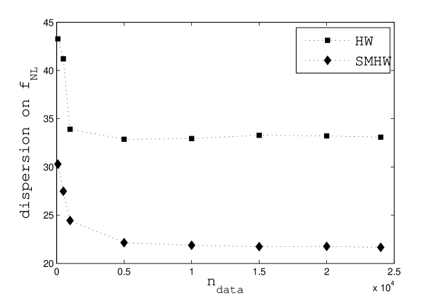
Figure 2: Results of the dispersion of $\hat{f}_{\rm NL}$ for 1000 Gaussian simulations for different values of $n_{\mathrm{data}}$.

4.3 Training evolution

Figure 3 illustrates the training evolution for the classification network with $n_{\rm hid}=0$ and $n_{\rm class}=9$. In the top two panels we plot the true positive rates (TPR) of the network on the training set and the test set, for the HW and SHMW respectively; in each plot, the TPR on the training set has been mutliplied by a factor less than unity to highlight the divergence with the TPR for the test set. We see that this divergence occurs after $\sim 100$ and $\sim 500$ iterations of the MemSys optimiser for the HW and SMHW, respectively. Thus the training was terminated at this point to construct our final classification networks.

A key criterion in determining the quality of our classifiers is the dispersion of the $f_{\rm NL}$ values obtained in the testing set. This is plotted in the bottom two panels of Figure 3 for the HW and SMHW, respectively. We note that, in each case, this dispersion increases noticeable beyond the point where the TPRs on the training and testing sets diverge.

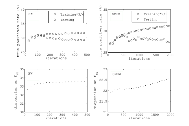
Figure 3: Evolution of the true positive rate for each iteration of the training process with a neural network with $n_{\mathrm{hid}}=0$ and $n_{\mathrm{data}}=10000$. Note that the TPR of the training set have been multiplied by a factor less than unity in order to highlight the divergence of the behaviours. The bottom panels show the variation of the dispersion on the estimate $\hat{f}_{\rm NL}$ during the training. Left panels for HW and right panels for SMHW.

5 Results

5.1 Application to WMAP simulations

We first applied our classifiers to 1000 WMAP-7yr simulations made from Gaussian CMB maps ($f_{\rm NL}=0$). For the HW classifier, we obtained $\langle\hat{f}_{\rm NL}\rangle=-1$, which indicates the estimator is essentially unbiassed. Moreover, the dispersion of the estimator $\sigma(\hat{f}_{\rm NL})=33$ is extremely similar to that obtained with the weighted least-squares method ($\sigma(\hat{f}_{NL})=34$). The full distribution of the estimator is shown in the top panel of Fig. 4. For the SMHW classifier, we again found $\langle\hat{f}_{\rm NL}\rangle=-1$, with a dispersion of $\sigma(\hat{f}_{\rm NL})=22$, which is very close to the optimal value of $\sigma(\hat{f}_{\rm NL})=21$. The distribution of the estimator for the SMHW is shown in the bottom panel of Fig. 4.

The histogram bins in Fig. 4 have the same size and central values as those used to define the network classes. We see that the classes at extremal $f_{\rm NL}$ values are empty, indicating that the network placed no maps in these $f_{\rm NL}$ ranges. Thus for estimating $f_{\rm NL}$ from Gaussian or nearly Gaussian maps the range in $f_{\rm NL}$ used is sufficiently wide.

We next applied our estimator to sets of non-Gaussian simulations, each with a different non-zero $f_{\rm NL}$ value. For each true $f_{\rm NL}$ value, we analysed the corresponding WMAP simulations and calculated the mean and dispersion of our estimator $\hat{f}_{\rm NL}$ for both the HW and SMHW classifiers. The results are shown in fig. 5, in which we plot the mean value of $\hat{f}_{\rm NL}$ against the true $f_{\rm NL}$ value. We see that the classifiers are unbiassed for $|f_{\rm NL}|\lesssim\sigma$ with an almost constant dispersion. For larger $|f_{\rm NL}|$ values, however, the estimator becomes progressively more biassed and its dispersion decreases.

The latter behaviour is simply understood as an edge effect due to the finite total range of $f_{\rm NL}$ considered by the networks. This point is illustrated in Fig. 6 in which we plot the full distributions of $\hat{f}_{\rm NL}$ obtained for a number of representative values of the true $f_{\rm NL}$. We see that for $|f_{\rm NL}|\lesssim\sigma$, we obtain close to symmetric distribution centred on the true $f_{\rm NL}$ value, with no maps being placed in the extreme classes. As $|f_{\rm NL}|>\sigma$, however, we see that the classifier does begin to place maps in the extreme classes, resulting in the distribution of $\hat{f}_{\rm NL}$ becoming severely skewed and no longer centred on the true value. Of course, if one were to encounter this behaviour in the analysis of a real data set, one could simply alter the range of $f_{\rm NL}$ considered by the network and retrain.

In any case, the above results show that both the HW and SMHW network classifiers produce unbiassed estimates $\hat{f}_{\rm NL}$ provided $-\sigma<f_{NL}<\sigma$. Moreover, the dispersions on these estimators are very similar to those obtained with the classical weighted least squares (WLS) method, indicating that neural networks can produce very accurate results within the limitations described above. In the case of the SMHW, this is a particularly important result since the complexity of the covariance matrix inversion required in the standard approach is bypassed via the use of the neural network classifier. Curto et al. (2011a) used a principal component analysis to reduce the covariance matrix dimension to allow inversion.

$\begin{array}[]{c}\includegraphics[width=142.26378pt,height=113.81102pt]{hist_HW_plus_rot_ndata10000.eps}\\ \includegraphics[width=142.26378pt,height=113.81102pt]{hist_SMHW_diff_noise_ndata10000.eps}\end{array}$

Figure 4: Distribution of $\hat{f}_{\rm NL}$ obtained from 1000 Gaussian realizations for HW (top) and SMHW (bottom).

$\begin{array}[]{c}\includegraphics[width=170.71652pt,height=113.81102pt]{fnl_fnlest_HW_large_range.eps}\\ \includegraphics[width=170.71652pt,height=113.81102pt]{fnl_fnlest_SMHW_large_range.eps}\end{array}$

Figure 5: The mean and dispersion of $\hat{f}_{\rm NL}$ obtained for a number of representative values of the true $f_{\rm NL}$ for the HW network (top) and the SMHW network (bottom).

	$\hat{f}^{\phantom{\int}}_{\rm NL,data}$	$\sigma(\hat{f}_{\rm NL})$	$\langle\hat{f}_{\rm NL,gauss}\rangle$	$P_{2.5}$	$P_{97.5}$
SMHW (NN)	19	22	$-1$	$-43$	42
SMHW (WLS)
Curto et al. 2011b	37	21	0	$-42$	46
HW (NN)	$-12$	33	$-1$	$-66$	63
HW (WLS)
Casaponsa et al. 2011	6	34	1	$-68$	67

Table 1: Results obtained with neural networks (NN) and weighted least squares (WLS). $\hat{f}_{\rm NL,data}$ is the best fitting value for V+W WMAP data, $\langle\hat{f}_{\rm NL,gauss}\rangle$ and $\sigma(\hat{f}_{\rm NL})$ are the expected value and the standard deviation for Gaussian simulations. $P_{2.5}$ and $P_{97.5}$ represent the percentile values at 95% confidence level of $\hat{f}_{\rm NL}$ for Gaussian realizations.

$\begin{array}[]{cc}\includegraphics[width=256.0748pt,height=199.16928pt]{histos_fnl_HW.eps}\includegraphics[width=256.0748pt,height=199.16928pt]{histos_fnl_SMHW.eps}\end{array}$

Figure 6: Distribution of $\hat{f}_{\rm NL}$ obtained from 200 non-Gaussian realizations with representative true $f_{\rm NL}$ values, for HW (left) and SMHW (right).

5.2 Application to WMAP 7-year data

Applying the neural network classifiers to real data (the V+W WMAP 7-year data map), we obtain $\hat{f}_{\rm NL}=-12$ for the HW and $\hat{f}_{\rm NL}=19$ for the SMHW. Both these values lie well within the corresponding dispersion of the estimator. From the corresponding $\hat{f}_{\rm NL}$ distributions obtained on simulated data, we find that 95% confidence limits are $-78<f_{\rm NL}<51$ for the HW and $-24<f_{\rm NL}<61$ for the SMHW. We therefore conclude that the data are consistent with the Gaussian hypothesis. We note that the SMHW confidence limits are very similar to those obtained with the optimal $f_{\rm NL}$ estimator (Komatsu et al., 2011; Smith et al., 2009).

These results are summarised in Table 1, along with found via the weighted least squares (WLS) method. The latter results are also consistent with Gaussianity. It is worth mentioning, however, the different values of $\hat{f}_{\rm NL}$ obtained by the neural network and the WLS methods, for both HW and SMHW. Although all four values lie well within their corresponding dispersions, each method returns a different $\hat{f}_{\rm NL}$ value when applied to the same WMAP-7yr dataset. This behaviour is to be expected, however, since these are four different estimators of $f_{\rm NL}$. Therefore, in general, they will not be equal, even when applied to the same input data. Only the statistical properties (e.g. mean, dispersion) of their sampling distributions are important.

6 Conclusions

We have trained a multi-class neural network classifier with third-order moments of the HW and SMHW coefficients of non-Gaussian realizations in order to set constraints on the local non-linear coupling term $f_{NL}$ using WMAP 7-year data. We found that with a very simple network and with few iterations (requiring just a few secs CPU time) it is possible to produce the same results as those obtained with the weighted least squares method. This is an interesting achievement, as it bypasses any covariance matrix related computations and their associated regularisation problems. The estimation of the covariance matrix with both wavelets requires the analysis of at least 10000 Gaussian simulations which involves a huge demand in CPU time, in particular with the SMHW statisitcs. The error bars on the estimation of $f_{\rm NL}$ computed with Gaussian simulations are $\sigma(\hat{f}_{NL}=33)$ for HW and $\sigma(\hat{f}_{NL})=22$ for SMHW, which are extremely similar to the ones obtained in Casaponsa et al. (2010) and Curto et al. (2011a) using the same statisitcs but a different estimator based on the weighted least squares method ($\sigma=34$, $\sigma=21$ for HW and SMHW respectively). The constraints for WMAP 7-year data were found to be $-78<f_{\rm NL}<51$ for the HW and $-24<f_{\rm NL}<61$ for the SMHW, which are compatible to a Gaussian distribution as found in Smith et al. (2009); Curto et al. (2009b); Komatsu et al. (2011); Casaponsa et al. (2010) and Curto et al. (2011b). The results obtained with the SMHW statistics are similar to the ones found in Smith et al. (2009) and Komatsu et al. (2011), which are the most stringent ones currently available at the limit of the WMAP resolution. Further analysis, as to the contribution to $f_{\rm NL}$ of unresolved point sources or foregrounds can be performed by applying the linear classifier to the statistics of new simulated maps with this characteristic signal.

References

- Antoine & Vandergheynst (1998) Antoine J.-P., Vandergheynst P., 1998, Journal of Mathematical Physics, 39, 3987
- Auld et al. (2007) Auld T., Bridges M., Hobson M. P., Gull S. F., 2007, MNRAS, 376, L11
- Babich et al. (2004) Babich D., Creminelli P., Zaldarriaga M., 2004, Journal of Cosmology and Astro-Particle Physics, 8, 9
- Baccigalupi et al. (2000) Baccigalupi C., Bedini L., Burigana C., De Zotti G., Farusi A., Maino D., Maris M., Perrotta F., Salerno E., Toffolatti L., Tonazzini A., 2000, MNRAS, 318, 769
- Barreiro et al. (2000) Barreiro R. B., Hobson M. P., Lasenby A. N., Banday A. J., Górski K. M., Hinshaw G., 2000, MNRAS, 318, 475
- Bartolo et al. (2004) Bartolo N., Komatsu E., Matarrese S., Riotto A., 2004, Phys.Rev.D, 402, 103
- Bucher et al. (2010) Bucher M., van Tent B., Carvalho C. S., 2010, MNRAS, 407, 2193
- Carballo et al. (2008) Carballo R., González-Serrano J. I., Benn C. R., Jiménez-Luján F., 2008, MNRAS, 391, 369
- Casaponsa et al. (2010) Casaponsa B., Barreiro R. B., Curto A., Martínez-González E., Vielva P., 2010, ArXiv e-prints
- Cayón et al. (2003) Cayón L., Martínez-González E., Argüeso F., Banday A. J., Górski K. M., 2003, MNRAS, 339, 1189
- Cayón et al. (2001) Cayón L., Sanz J. L., Martinez-Gonzalez E., Banday A. J., Argueso F., Gallegos J. E., Gorski K. M., Hinshaw G., 2001, MNRAS, 326, 1243
- Cruz et al. (2005) Cruz M., Martínez-González E., Vielva P., Cayón L., 2005, MNRAS, 356, 29
- Curto et al. (2009b) Curto A., Martínez-González E., Barreiro R. B., 2009b, ApJ, 706, 399
- Curto et al. (2011a) Curto A., Martinez-Gonzalez E., Barreiro R. B., 2011a, MNRAS, 412, 1023
- Curto et al. (2011b) Curto A., Martinez-Gonzalez E., Barreiro R. B., Hobson M. P., 2011b, submitted to MNRAS
- Curto et al. (2009a) Curto A., Martínez-González E., Mukherjee P., Barreiro R. B., Hansen F. K., Liguori M., Matarrese S., 2009a, MNRAS, 393, 615
- Elsner & Wandelt (2009) Elsner F., Wandelt B. D., 2009, ApJS, 184, 264
- Elsner & Wandelt (2010) Elsner F., Wandelt B. D., 2010, ApJ, 724, 1262
- Fergusson et al. (2010) Fergusson J. R., Liguori M., Shellard E. P. S., 2010, Physical Review D, 82, 023502
- Fergusson & Shellard (2009) Fergusson J. R., Shellard E. P. S., 2009, Phys. Rev. D, 80, 043510
- Gangui et al. (1994) Gangui A., Lucchin F., Matarrese S., Mollerach S., 1994, ApJ, 430, 447
- Górski et al. (2005) Górski K. M., Hivon E., Banday A. J., Wandelt B. D., Hansen F. K., Reinecke M., Bartelmann M., 2005, ApJ, 622, 759
- Gull & Skilling (1999) Gull S. F., Skilling J., 1999, Quantified maximum entropy: Mem-Sys 5 users’ manual. Maximum Entropy Data Consultants Ltd, Royston
- Hikage et al. (2008) Hikage C., Matsubara T., Coles P., Liguori M., Hansen F. K., Matarrese S., 2008, MNRAS, 389, 1439
- Hobson & Lasenby (1998) Hobson M., Lasenby A., 1998, 298, 905
- Jaynes (2003) Jaynes E., 2003, Probability Theory: The Logic of Science. Cambridge University Press
- Komatsu et al. (2011) Komatsu E., Smith K. M., Dunkley J., Bennett C. L., Gold B., Hinshaw G., Jarosik N., Larson D., Nolta M. R., Page L., Spergel D. N., Halpern M. an Wright E. L., 2011, ApJS, 192, 18
- Komatsu & Spergel (2001) Komatsu E., Spergel D., 2001, Phys.Rev.D, 63, 063002
- Komatsu et al. (2005) Komatsu E., Spergel D. N., Wandelt B. D., 2005, ApJ, 634, 14
- Leshno et al. (1993) Leshno M., V. Y., A. P., Schocken S., 1993, Neural Netw., 6, 861
- MacKay (2003) MacKay D., 2003, Information Theory, Inference and Learning Algorithms. Cambridge University Press
- Martínez-González et al. (2002) Martínez-González E., Gallegos J. E., Argueso F., Cayon L., Sanz J. L., 2002, MNRAS, 336, 22
- McEwen et al. (2008) McEwen J. D., Hobson M. P., Lasenby A. N., Mortlock D. J., 2008, MNRAS, 388, 659
- McEwen et al. (2007) McEwen J. D., Vielva P., Wiaux Y., Barreiro R. B., Cayon L., Hobson M. P., Lasenby A. N., Martinez-Gonzalez E., Sanz J. L., 2007, Journal of Fourier Analysis and Applications, 13, 495
- Mukherjee & Wang (2004) Mukherjee P., Wang Y., 2004, ApJ, 613, 51
- Natoli et al. (2010) Natoli P., de Troia G., Hikage C., Komatsu E., Migliaccio M., Ade P. A. R., Bock J. J., Bond J. R., Borrill J., Boscaleri A., Contaldi C. R., Crill B. P., de Bernardis P., de Gasperis G., de Oliveira-Costa A., di Stefano G., Hivon E., 2010, MNRAS, 408, 1658
- Pietrobon (2010) Pietrobon D., 2010, Memorie della Societa Astronomica Italiana Supplementi, 14, 278
- Salopek & Bond (1990) Salopek D. S., Bond J. R., 1990, Phys.Rev.D, 42, 3936
- Shahram et al. (2007) Shahram M., Donoho D., Starck J., 2007, in Society of Photo-Optical Instrumentation Engineers (SPIE) Conference Series Vol. 6701 of Society of Photo-Optical Instrumentation Engineers (SPIE) Conference Series, Multiscale representation for data on the sphere and applications to geopotential data
- Smith et al. (2009) Smith K. M., Senatore L., Zaldarriaga M., 2009, Journal of Cosmology and Astro-Particle Physics, 9, 6
- Storrie-Lombardi et al. (1992) Storrie-Lombardi M. C., Lahav O., Sodre Jr. L., Storrie-Lombardi L. J., 1992, MNRAS, 259, 8P
- Tenorio et al. (1999) Tenorio L., Jaffe A. H., Hanany S., Lineweaver C. H., 1999, MNRAS, 310, 823
- Vanzella et al. (2004) Vanzella E., Cristiani S., Fontana A., Nonino M., Arnouts S., Giallongo E., Grazian A., Fasano G., Popesso P., Saracco P., Zaggia S., 2004, A&A, 423, 761
- Verde et al. (2000) Verde L., Wang L., Heavens A. F., Kamionkowski M., 2000, MNRAS, 313, 141
- Vielva et al. (2004) Vielva P., Martinez-Gonzalez E., Barreiro R. B., Sanz J. L., Cayon L., 2004, ApJ, 609, 22
- Vielva & Sanz (2010) Vielva P., Sanz J. L., 2010, MNRAS, 404, 895
- Yadav & Wandelt (2010) Yadav A. P. S., Wandelt B. D., 2010, Advances in Astronomy, 2010