Mixed modes in red-giant stars observed with CoRoT

Abstract

Context. The CoRoT mission has provided thousands of red-giant light curves. The analysis of their solar-like oscillations allows us to characterize their stellar properties.

Aims. Up to now, the global seismic parameters of the pressure modes remain unable to distinguish red-clump giants from members of the red-giant branch. As recently done with Kepler red giants, we intend to analyze and use the so-called mixed modes to determine the evolutionary status of the red giants observed with CoRoT. We also aim at deriving different seismic characteristics depending on evolution.

Methods. The complete identification of the pressure eigenmodes provided by the red-giant universal oscillation pattern allows us to aim at the mixed modes surrounding the $\ell$=1 expected eigenfrequencies. A dedicated method based on the envelope autocorrelation function is proposed to analyze their period separation.

Results. We have identified the mixed-mode signature separation thanks to their pattern compatible with the asymptotic law of gravity modes. We have shown that, independent of any modelling, the g-mode spacings help to distinguish the evolutionary status of a red-giant star. We then report different seismic and fundamental properties of the stars, depending on their evolutionary status. In particular, we show that high-mass stars of the secondary clump present very specific seismic properties. We emphasize that stars belonging to the clump were affected by significant mass loss. We also note significant population and/or evolution differences in the different fields observed by CoRoT.

1 Introduction

The CoRoT and Kepler missions have revealed solar-like oscillation in thousands of red-giant stars. This gives us the opportunity to test this important phase of stellar evolution, and provides new information in stellar and galactic physics (2009A&A...503L..21M; 2011Natur.471..608B). Thanks to the dramatic increase of information recently made available (2009Natur.459..398D; 2009A&A...506..465H; 2010A&A...517A..22M; 2010A&A...522A...1K; 2010ApJ...723.1607H), we have now a precise view of pressure modes (p modes) corresponding to oscillations propagating essentially in the large convective envelopes. Gravity modes (g modes) may exist in all stars with radiative regions. They result from the trapping of gravity waves, with buoyancy as a restoring force. In red giants, gravity waves propagating in the core have high enough frequencies to be coupled to pressure waves propagating in the envelope (2009A&A...506...57D). The trapping of such waves with mixed pressure and gravity character gives the so-called mixed modes. The coupling insures non-negligible oscillation amplitudes in the stellar photosphere, hence the possible detection of these mixed modes.

Observationally, mixed modes were first identified in white-dwarf oscillation spectra (1991ApJ...378..326W). They have also been observed in sub-giant stars, first with ground-based observations (2005A&A...434.1085C; 2007ApJ...663.1315B; 2010ApJ...713..935B), then recently in Kepler and CoRoT fields (2010ApJ...713L.169C; 2010A&A...515A..87D). In red giants, they were first suspected by 2010ApJ...713L.176B. Their presence significantly complicates the fit of the p modes observed in CoRoT giants (2010A&A...520A..60H; 2010AN....331.1016B) and they were identified as outliers to the universal red-giant oscillation spectrum (2011A&A...525L...9M). Recent modelling of a giant star observed by the Kepler mission had to take their presence into account (2011arXiv1105.1076D). Finally, they have been firmly identified in Kepler data (2011Sci...332..205B), making the difference clear between giants burning hydrogen in shell or helium in the core (2011Natur.471..608B).

The theoretical analysis of these mixed modes in red giants has been performed prior to observations (2001MNRAS.328..601D; 2004SoPh..220..137C; 2009A&A...506...57D). Using a non-radial non-adiabatic pulsation code including a non-local time-dependent treatment of convection and a stochastic excitation model, 2009A&A...506...57D have computed the eigenfrequencies and the mode heights in several red-giant models. They have shown that mixed modes have much larger mode inertias than p modes, hence present longer lifetimes and smaller linewidths. They were able to identify different regimes, depending on the location of the models on the red-giant branch. Recently, 2010ApJ...721L.182M proposed to use the oscillation spectrum of dipole modes to discriminate between red-giant branch (RGB) and central-He burning (clump) evolutionary phase of red giants. This illustrates the fact that observing p-g-mixed modes and identifying their properties give us a unique opportunity to analyze the cores of red giants, since the g component is highly sensitive to the core condition (2009A&A...506...57D).

In this paper, we present and validate an alternative method to 2011Natur.471..608B to detect and identify mixed modes in red giants. We use it to analyze red-giant stars in two different fields observed by CoRoT and show that they present different properties: mixed modes do not only allow us to distinguish different evolutionary status, they can also show different population characteristics. We also assess clear observational differences between the fundamental and seismic properties of the red-giant stars, depending on their evolutionary status. We show for instance that the observation of mixed modes opens a new way to study the mass loss at the tip of the RGB. We have also clear indication that mixed modes in red giants are sensitive to chemical composition gradients in the deep interior, as they are in SPB and $\gamma$ Doradus stars (2008MNRAS.386.1487M). Their study will definitely boost both stellar and galactic physics.

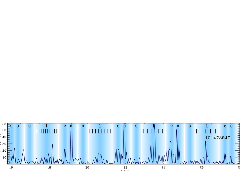
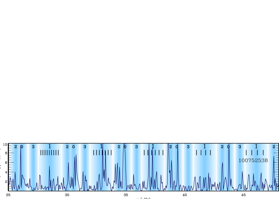
Figure 1: Shaded regions of these bar code spectra reproduce the universal red-giant oscillation pattern and identify the location of the different harmonic degrees for three CoRoT targets (ID given on the right side); the more dense the background, the higher the probability to have the short-lived p mode realized there. Black dashes in the $\ell=1$ ridges indicate the asymptotic spacing of the mixed modes as derived from Eq. 2; they do not give their exact eigenfrequencies, since the asymptotic relation does not account for the mode bumping of mixed modes.

2 Analysis

2.1 Mixed-mode pattern

According to 2009A&A...506...57D, each $\ell=1$ ridge is composed of a pressure mode surrounded by mixed modes with a pattern mostly dominated by the g-mode component. According to the asymptotic description (1980ApJS...43..469T), both p modes and g modes present well organized patterns. For p modes, the organization is a comb-like structure in frequency, for g modes, regularity is observed in period. Mixed modes in giants are supposed to exhibit the well-organized pattern of g modes. In order to detect them in an automated way, we have searched for this asymptotic pattern:

$$T_{n_{\mathrm{g}},\ell}={2\pi^{2}(n_{\mathrm{g}}+\alpha_{\ell})\over\sqrt{\ell(\ell+1)}}\ \left[\int_{\mathrm{core}}\!\!{{N_{\mathrm{BV}}\over r}\;\mathrm{d}r}\right]^{-1}={(n_{\mathrm{g}}+\alpha_{\ell})\ \Delta T_{\mathrm{g}}\over\sqrt{\ell(\ell+1)}}$$ (1)

with $n_{\mathrm{g}}$ the gravity radial order, $\alpha_{\ell}$ an unknown constant and $N_{\mathrm{BV}}$ the Brunt-Väisälä frequency. The period spacing $\Delta T_{\mathrm{g}}$ is the equivalent for g modes of the large separation for p modes.

2.2 Periodic spacings

We have first restricted our attention to $\ell=1$ modes since mixed modes with $\ell=2$ are not supposed to be as clearly visible (2009A&A...506...57D). Furthermore, the close proximity of $\ell=2$ modes to radial modes complicates the analysis. For the $\ell=1$ mixed modes, the periodic pattern simply becomes:

$$T_{n_{\mathrm{g}},1}=\left[n_{\mathrm{g}}+\alpha_{1}\right]\Delta T_{1},\hbox{ with \ }\Delta T_{1}=\Delta T_{\mathrm{g}}/\sqrt{2}.$$ (2)

The period spacing $\Delta T_{1}$, linked to the integral of the Brunt-Väisälä frequency by Eq. 1, can be deduced from the frequency spacing in the Fourier spectrum. To measure this spacing, we need to focus on the mixed modes. We are able to do this using the method introduced in 2011A&A...525L...9M which allows for a complete and automated mode identification. We then use the envelope autocorrelation function (2009A&A...508..877M) to derive the period spacing. The method is described in the Appendix. As for the method presented by 2011Natur.471..608B, it derives a period $\Delta T_{\mathrm{obs}}$ less than $\Delta T_{1}$, due to the bumping of mixed modes. We have estimated that, for the 5-month long CoRoT time series, we measure $\Delta T_{\mathrm{obs}}\simeq\Delta T_{1}/1.15$ (see Appendix).

Table 1: Typical parameters of mixed modes

$\langle\Delta\nu\rangle$	$\nu_{\mathrm{max}}$	$\delta\nu_{\mathrm{env}}$	$\Delta T_{\mathrm{obs}}$	$\Delta T_{1}$ proxy	$n_{\mathrm{g}};\Delta n_{\mathrm{g}}$	$n_{\mathrm{g}};\Delta n_{\mathrm{g}}$	$n_{\mathrm{g}};\Delta n_{\mathrm{g}}$	$\mathcal{T}$
					at $\nu_{\mathrm{max}}-\delta\nu_{\mathrm{env}}/2$	at $\nu_{\mathrm{max}}$	at $\nu_{\mathrm{max}}+\delta\nu_{\mathrm{env}}/2$
$\mu$Hz	$\mu$Hz	$\mu$Hz	s	s				day
Red-clump stars
4.0	32	13	250	287	137; 5	108; 3	89; 2	78
7.0	73	28	150	173	97; 3	78; 2	66; 1	25
Red-giant branch stars
2.5	19	8	800	920	73; 3	57; 2	46; 1	70
4.0	32	13	80	92	429;17	339;10	281; 7	245
6.0	60	23	60	69	300; 9	241; 6	201; 4	93
9.0	102	38	60	69	174; 5	142; 3	119; 2	32

The frequency $\nu_{\mathrm{max}}$ corresponds to the maximum oscillation signal; $\delta\nu_{\mathrm{env}}$ indicates the full width at half-maximum of the observed excess oscillation power (2010A&A...517A..22M). The proxies of the period spacing $\Delta T_{1}$ are estimated as $1.15\,\Delta T_{\mathrm{obs}}$. The values of $n_{\mathrm{g}}$ are derived from Eq. 2, with the parameter $\alpha_{\ell=1}=0$. $\Delta n_{\mathrm{g}}$ corresponds to the maximum number of observable mixed modes in a $0.25\,\Delta\nu$-wide interval around each pure p mode. $\mathcal{T}$ indicates the observational length required to measure the g-mode spacing according to the Shannon criterion.

2.3 Positive detection

The analysis has been performed on CoRoT red giants previously analyzed in 2009A&A...506..465H and 2010A&A...517A..22M. These stars were observed continuously during 5 months in 2 different fields respectively centered on the Galactic coordinates (37^∘, $-07^{\circ}$45′) and (212^∘, $-01^{\circ}$45′). Targets with a too low signal-to-noise ratio were excluded (see the Appendix). We therefore only considered stars with accurate global seismic parameters and labelled as the $\mathcal{N}_{3}$ set in 2010A&A...517A..22M.

Thanks to the method exposed in the Appendix, we have analyzed all red-giant spectra in an automated way. We have then checked all results individually. This allowed us to discard a few false positive results, and then to verify that the asymptotic expansion of the g modes (Eq. 2) gives an accurate description of the mixed modes since it is able to reproduce their spacings. The irregularities of the spacings are discussed in Section 3.1 and in the Appendix. A few examples are given in Fig. 1: we have overplotted on red-giant oscillation spectra the expected location of the p-mode pattern derived from 2011A&A...525L...9M and we have indicated the frequency separation of the mixed modes derived from the asymptotic description. Because of the mode bumping due to the coupling, the g-mode asymptotic expression is not able to derive the exact location of the mixed-mode eigenfrequencies, but we see that the spacings reproduce the observations. This agreement is certainly related to the fact that, according to Eq. 2, very high values of the gravity radial orders are measured, typically above 60 and up to 400 (Table 1). We were then able to provide a diagram representing the period separation $\Delta T_{\mathrm{obs}}$ of the mixed modes as a function of the large frequency separation $\Delta\nu$ of the pressure modes (Fig. 2).

The 5-month long CoRoT time series provide a frequency resolution of about 0.08 $\mu$Hz, accurate enough for detecting the mixed-modes in the red clump but limiting their possible detection at lower frequency. Therefore, we have taken care of possible artefacts. We have excluded the region of the $\langle\Delta\nu\rangle$ - $\Delta T_{\mathrm{obs}}$ diagram limited by the frequency resolution (Fig. 2). We have also taken care of the possible confusion with the small separation $\delta\nu_{02}$, since in given frequency ranges its signature can mimic a g-mode spacing (dotted line in Fig. 2). Due to the low visibility of $\ell=3$ modes, it appeared useless to test the influence of their pattern combined with radial or dipole modes.

The criterion of a positive detection of the mixed modes in at least two frequency ranges allowed us to discriminate regular period spacings from regular frequency spacings as caused by rotation. We also examined the possible confusion with the ragged, speckle-like, appearance of the structure due to the limited lifetime of the modes. Simulations have shown that the threshold level provided by the method (2009A&A...508..877M) combined with the detection in multiple frequency ranges excludes spurious signature.

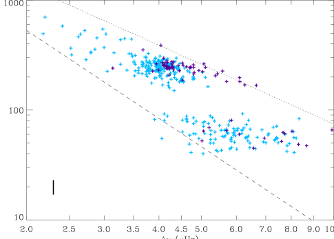
Figure 2: Period separation of mixed modes $\Delta T_{\mathrm{obs}}$ as a function of the mean frequency separation of the pressure modes $\langle\Delta\nu\rangle$. Blue (purple) crosses represent the targets observed in the center (anticenter) direction. The dashed line indicates the frontier below which the frequency resolution is not fine enough for deriving $\Delta T_{\mathrm{obs}}$ and the dotted line represents the location of the spurious signature that would correspond to the small separation $\delta\nu_{02}$ (2011A&A...525L...9M). The two separate domains correspond to the location of $\Delta T_{1}$ expected by josefina and observed by 2011Natur.471..608B. The vertical thick line indicates the mean 1-$\sigma$ error bars (the error bar on the large separation $\Delta\nu$ is in fact very small).

Finally, we have identified an $\ell=1$ mixed-modes pattern in about 42 % of the targets (387 out of a total of 929), and for more than 75 % of the stars with a R magnitude brighter than 13. The few remaining bright stars do not present a reliable signature, either because their spectrum is free of mixed modes, or because the signature was not found reliable according to the threshold detection level. When detected, the pattern follows closely both the asymptotic expression of gravity modes (1980ApJS...43..469T) and the description made by 2009A&A...506...57D. The peaks generating these spacings are visible in a frequency range of about $0.25\,\Delta\nu$ around the expected pure p-mode eigenfrequencies $\nu_{n,1}$. This represents typically, at the peak of the red clump distribution ($\Delta\nu\simeq 4\ \mu$Hz and $\nu_{\mathrm{max}}\simeq 32\,\mu$Hz), from two to ten mixed modes (Table 1). Due to the frequency dependence derived from Eq. 2, the number of observable modes varies very rapidly, as observed by 2011Sci...332..205B and made explicit in Table 1.

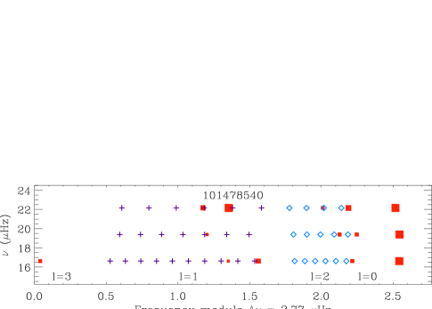
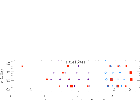
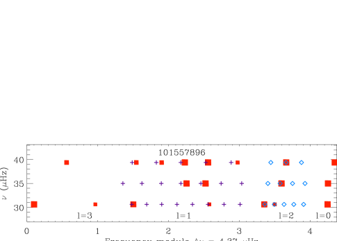
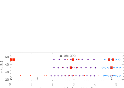
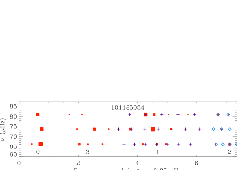
Figure 3: Échelle diagrams around $\nu_{\mathrm{max}}$ for different targets sorted by increasing large separations. The red squares indicate the observed peaks, selected with a height-to-background ratio above 6. Dark blue crosses indicate the expected location of the $\ell=1$ mixed modes strictly following the asymptotic expression; light blue diamonds are for $\ell=2$. Similarly to Fig. 1, crosses and diamonds indicate the mean spacing of the mixed modes only, not their exact location.

According to 2009A&A...506...57D, $\ell=2$ mixed modes are expected to be much more damped than $\ell=1$ modes. However, their presence is clearly identified for about a third of the targets (Fig. 3). The agreement of their mean separation with $\Delta T_{2}\simeq\Delta T_{1}/\sqrt{3}$ (Eq. 1) is clear enough to be disentangled from the speckle-like aspect of short-lived modes. Their observation will give strong constraints on the inner envelope, where g modes are coupled to p modes, the coupling being highly sensitive to the respective location of the Brunt-Väisälä and $\ell=2$ Lamb frequency. The high density of mixed modes, due to the high values of the radial gravity orders observed, makes it possible to achieve this high-resolution analysis. We observe in most cases groups of only two $\ell=2$ mixed modes, rarely three, spread in a frequency range of about $0.04\,\Delta\nu$. A further consequence of the observation of $\ell=2$ mixed modes is a correction to the asymptotic laws reported for the small separation $\delta\nu_{02}$ by 2010ApJ...723.1607H and 2011A&A...525L...9M; they are correct, but only indicative of the barycenter of the $\ell=2$ modes, if mixed.

3 Discussion

3.1 Period spacing

The measurement of mixed-mode spacings varying as $1/\nu^{2}$ (Eq. LABEL:spacing) validates the use of the asymptotic law of g modes, even if a detailed view of the mixed modes indicates irregularities in their spacings (Fig. 3). These shifts may be interpreted as a modulation due to the structure of the core with a sharp density contrast compared to the envelope, as observed in white dwarfs. The determination of $\Delta T_{1}$ will allow modelers to define the size of the radiative core region. The direct measurement of the individual shifts $\Delta T_{1}(n_{\mathrm{g}})$ will give access to the core stratification (2008MNRAS.386.1487M), as well as the observation (or not) of $\ell=2$ mixed modes that test a different cavity.

The method developed in this paper presents many interesting characteristics compared to the method used by 2011Natur.471..608B. First, it is directly applicable in the Fourier spectrum and does not require the power spectrum to be expressed in period. The method is fully automated, since it is coupled to the identification of the spectrum based on the universal pattern, and it includes a systematic search of periodic spacings that are not related to the p-mode pattern. Based on an $H_{0}$ test, it intrinsically includes a statistical test of reliability. This test defines a threshold level that makes the method efficient even at low signal-to-noise ratio. Its most interesting property certainly consists in its ability to derive the measurement of the variation of $\Delta T_{1}$ with frequency, as the EACF method used for p modes (2009A&A...508..877M; 2010AN....331..944M). In fact, the method was developed in parallel to the one mainly presented in 2011Natur.471..608B, and gave similar results that confirmed the detection of mixed modes in Kepler giants.

3.2 Red-clump and red-giant branch stars

Red-clump stars have been characterized in previous work (e.g. Fig. 5 of 2010A&A...517A..22M). They contribute to a distribution in $\Delta\nu$ with a pronounced accumulation near 4 $\mu$Hz (equivalent to the accumulation near $\nu_{\mathrm{max}}\simeq 32\,\mu$Hz). However, population analysis made by 2009A&A...503L..21M has shown that this population of stars with $\Delta\nu\simeq 4\,\mu$Hz effectively dominated by red-clump stars also contains a non-negligible fraction ($\simeq 30$ %) of RGB stars. None of the global parameters of p mode (neither $\Delta\nu$ nor $\nu_{\mathrm{max}}$) is able to discriminate between RGB and red-clump stars. However, as shown by 2011Natur.471..608B with Kepler data, the examination of the relation between the p-mode and g-mode spacings shows two regimes (Fig. 2). The signature of the red-clump stars piling up around $\langle\Delta\nu\rangle\simeq 4\,\mu$Hz is visible with $\Delta T_{\mathrm{obs}}\simeq 250$ s. Another group of stars has $\Delta T_{\mathrm{obs}}$ values lower than 100 s. Regardless of any modelling, this gives a clear signature of the difference between red-clump stars that burn helium in their core and stars of the red-giant branch that burn hydrogen in a shell (2010ApJ...721L.182M). The agreement with theoretical values is promising (josefina).

The contribution of the red-clump stars in the $\Delta\nu$-$\Delta T_{\mathrm{obs}}$ diagram presented in Fig. 2 is unambiguous. Stars with large separation larger than the clump value (about 4 $\mu$Hz) are located on the ascending red-giant branch or members of the secondary clump (1999MNRAS.308..818G; 2009A&A...503L..21M). At lower frequency than the clump, using mixed modes to disentangle the evolutionary status is more difficult. According to the identification of the clump provided by the distributions of the large separation (2010A&A...517A..22M), we assume that the giants with $\Delta\nu\leq 3.5\,\mu$Hz and $\Delta T_{\mathrm{obs}}\geq 200$ s belong to the RGB. The following analysis shows further consistent indications.

We finally note that the detection of RGB stars having a large separation similar to the peak of the clump stars ($\simeq 4\,\mu$Hz) is only marginally possible, due to insufficient frequency resolution. According to Table 1, more than 200 days are necessary to resolve the mixed modes, while CoRoT runs are limited to about 150 days.

3.3 Mode lifetimes and heights

We have remarked that, as predicted by 2009A&A...506...57D, the lifetimes of the mixed modes trapped in the core are much larger than the lifetimes of radial modes (Fig. 1). In most cases, the mixed modes are not resolved. When the mixed modes are identified, they corresponds in most cases to a comb-like pattern of thin peaks, without a larger and broader peak that could correspond to the pure $\ell=1$ pressure mode. However, since the detection of mixed modes is only achieved for a limited set of stars, one cannot exclude that some red giants only show pure $\ell=1$ pressure modes.

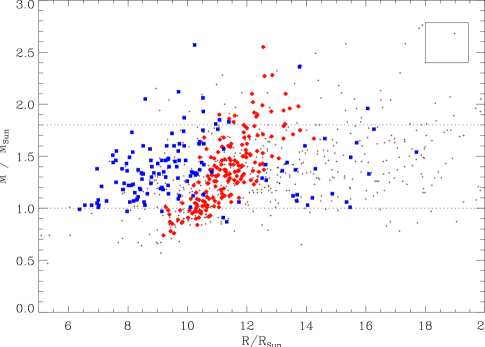
Figure 4: Asteroseismic mass as a function of the asteroseismic radius, with indication of the evolutionary status derived from the mixed-mode spacing: blue squares for RGB stars, red diamonds for clump stars; stars without clear measurement of $\Delta T_{\mathrm{obs}}$ are marked with a small cross. The rectangle indicates the mean 1-$\sigma$ error bars. The dotted lines at respectively 1 and 1.8$\,M_{\odot}$ correspond to the limits defined in the text.

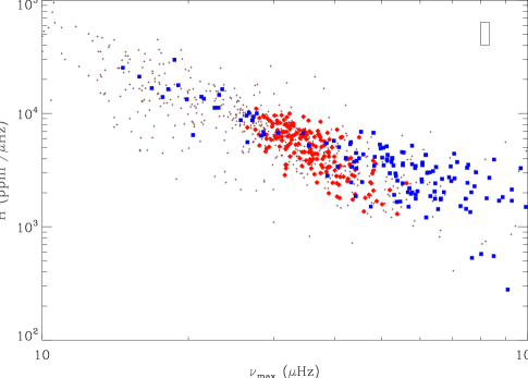
Figure 5: Mean mode height as a function of $\nu_{\mathrm{max}}$. Same color code as in Fig. 4. The rectangle indicates the mean 1-$\sigma$ error bars.

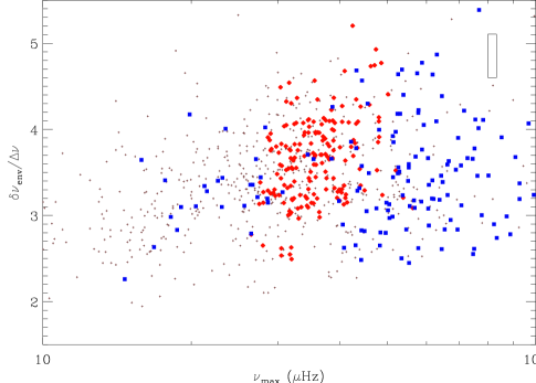
Figure 6: Proxy of the number of observable modes, given by the ratio $\delta\nu_{\mathrm{env}}/\Delta\nu$, as a function of $\nu_{\mathrm{max}}$. Same color code as in Fig. 4. The rectangle indicates the mean 1-$\sigma$ error bars.

3.4 Mass-radius relation

The possibility to distinguish the evolutionary status allows us to refine the ensemble asteroseismic analysis made on CoRoT red giants, especially the mass and radius distributions (Fig. 12 and 13 of 2010A&A...517A..22M). Benefitting from the same calibration of the asteroseismic mass and radius determination as done in this work, we have investigated the mass-radius relation, having in mind that without information of the evolutionary status, there is no clear information (2011MNRAS.tmp..559H).

We note here that the mass distribution is almost uniform in the RGB, contrary to clump stars (Fig. 4). The number of high-mass stars in the RGB, above $1.8\,M_{\odot}$ as defined in 2011Natur.471..608B, is about half of that in the clump, consistent with their expected more rapid evolution. Similarly, stars with masses below $1\,M_{\odot}$ are significantly rarer (by a factor of six to one) in the RGB by comparison with the clump. If we assume that the scaling relations, valid along the whole evolution from the main sequence to the giant class, remain valid after the tip of the RGB, this comparative study proves that low-mass stars present in the clump but absent in the branch have lost a substantial fraction of their mass due to stellar winds when ascending up to the tip of the RGB. Therefore, after the helium flash, these stars show lower mass. The quantitative study of this mass loss will require a careful unbiased analysis, out of the scope of this paper. On the contrary, high-mass stars, even if they lost mass too, can be observed as clump stars since they spend a much longer time in the core-helium burning phase than while ascending the RGB. Most of these stars belong to the secondary red clump (1999MNRAS.308..818G; 2011Natur.471..608B). We note that the secondary-clump stars present a larger spread in the mass-radius distribution, certainly due to the fact that those stars that have not undergone the helium flash present different interior structures. On the other side, the low-mass stars of the clump present a clear mass-radius relation: the helium flash shall have made their core largely homologous.

3.5 Mode amplitudes and number of modes

We can also address the influence of the evolutionary status on the energetic parameters of the red-giant oscillation spectrum. When plotting the mean height of the excess power Gaussian envelope as a function of the frequency $\nu_{\mathrm{max}}$, we remark that clump stars and RGB stars present very similar height for $\nu_{\mathrm{max}}$ less than 40 $\mu$Hz. However, above 40 $\mu$Hz, the oscillations in clump stars present systematically lower heights than RGB stars (Fig. 5). The contrast is more than a factor of 2. On the other side, the number of modes, estimated from the ratio $\delta\nu_{\mathrm{env}}/\Delta\nu$ where $\delta\nu_{\mathrm{env}}$ is the full width at half-maximum of the total oscillation excess power envelope, is similar below 40 $\mu$Hz, but more than 30 % larger for clump stars above this limit (Fig. 6). Despite the somewhat arbitrary limit in $\nu_{\mathrm{max}}$ we see here evidence of the secondary clump (1999MNRAS.308..818G), which consists of He-core burning stars massive enough to have ignited He in non-degenerate conditions. These stars have, at $\nu_{\mathrm{max}}>40\,\mu$Hz, similar radii as RGB stars, and larger masses. Hence, they have a smaller $L/M$ ratio, so that the excitation of oscillation is expected to be weaker. With a larger $\nu_{\mathrm{max}}$, they also present a solar-like oscillation spectrum with modes excited in a broader frequency range.

We suggest that, in case the measurement of $\Delta T_{\mathrm{obs}}$ is made difficult by a low signal-to-noise ratio, the oscillation amplitude and the size of the Gaussian envelope with noticeable amplitude may be used to help the determination of the evolutionary status.

Finally, we note that the secondary-clump population is certainly underestimated, owing to the fact that the low amplitudes make their detection quite complex in CoRoT data. In fact, such stars are observed with a low signal-to-noise ratio since their Fourier spectra are dominated by a white-noise contribution.

3.6 Different populations

The number of detections of solar-like oscillation towards the anticenter direction is lower than towards the center, due to a lower red-giant density in the outer galactic regions and to dimmer magnitudes (2010A&A...517A..22M). Hence, the number of reliable measurements of $\Delta T_{\mathrm{obs}}$ is lower too, but with the same proportion of 40 %. The sample is large enough to make sure that the difference between the distributions is significant (Fig. 2).

The anticenter field shows a significant deficit of red-clump stars below $\Delta\nu=3.8\,\mu$Hz, e.g. with small mass. Another similar deficit is observed at low frequency in the red-giant branch; it should indicate populations with different ages. We also note that secondary-clump stars of the anticenter direction present slightly higher g-mode spacings; it should indicate populations with different mass distributions. This illustrates the interest to compare the different fields in order to analyze different populations (Miglio et al., in preparation).

4 Conclusion

The clear identification of the p-mode oscillation pattern has allowed us to identify in CoRoT observations the pattern of mixed modes behaving as gravity modes in the core and pressure modes in the envelope. We have verified that this pattern is very close to the asymptotic expression of g modes. Benefitting from the identification of $\ell=1$ mixed modes, we also have measured $\ell=2$ mixed modes. The presence or absence of these mixed modes will allow us to study the deep envelope surrounding the core.

We have verified that the mean large period separation of the mixed modes gives a clear indication of the evolution of the star. Assuming the validity of the asteroseismic scalings laws for the stellar mass and radius, we have shown that the mass distribution of the RGB is much more uniform than in the red clump. Asteroseismology confirms that these red-clump stars have undergone a significant mass loss. Furthermore, red-giant low-mass stars after the helium flash do present homologous interiors and a clear mass-radius relation, contrary to stars in the secondary clump. Longer time series recorded with Kepler will allow us to investigate this relation in more detail. Benefitting from the fact that CoRoT provides observations in two fields, towards the Galactic center and in the opposite direction, we have now a performing indicator for making the population study more precise. This will be done in future work.

These data confirm the power of red-giant asteroseismology: we have access to the direct measure of the radiative central regions. Even if observations only deliver a proxy of the large period separation, comparison with modelling will undoubtedly be very fruitful. In a next step, the dedicated analysis of the best signal-to-noise ratio targets will allow us to sound in detail the red-giant core. Modulation of the large period spacing, observed in many targets, will give a precise view of the core layers.

Appendix A Method

Figure 7: Zoom on the bar code spectrum of the target CoRoT 100752538, with the large separation provided by the adjustment derived from the red-giant oscillation universal pattern. Different narrow filters centered on different pure $\ell=1$ pressure modes are indicated with different line styles. They allow us to measure a local g-mode frequency spacing in each filter.

Identifying $\ell=1$ mixed modes first requires to aim at them precisely. This first step is achieved by the method presented in 2011A&A...525L...9M, able to mitigate the major sources of noise that perturb the measurement of the large separation $\Delta\nu$ and then to derive the complete identification of the p-mode oscillation pattern. Complete identification means that all eigenfrequencies, their radial order and their degree, are unambiguously identified, as for instance the expected frequencies of the pure pressure $\ell=1$ modes:

$$\nu_{n,\ell=1}=[n+1/2+\varepsilon(\Delta\nu)-d_{01}]\;\Delta\nu,$$ (3)

with $\varepsilon(\Delta\nu)$ representing the surface term and $d_{01}$ accounting for the small separation of $\ell=1$ pure p modes.

Figure 8: Mean period spacings measured around the expected pure $\ell=1$ pressure modes of the target CoRoT 100752538. Vertical lines indicate the error bars on each individual measurement.

The frequency spacings of the mixed modes are then analyzed with the envelope autocorrelation function (EACF) based on narrow filters centered on the frequencies $\nu_{n,1}$ in the vicinity of the frequency $\nu_{\mathrm{max}}$ of maximum oscillation amplitude (2009A&A...508..877M). We deliberately chose the EACF method since it has proved to be efficient at very low signal-to-noise ratio (2009A&A...506...33M; 2010A&A...524A..47G; 2011A&A...525A.131H), thanks to a statistical test of reliability based on the null hypothesis.

In order to only select mixed modes, the full width at half-maximum of the filter is fixed to $\Delta\nu/2$ (Fig. 7). From the differentiation of the relation between period and frequency, the regular spacing of Eq. 2 in period translates into spacings varying with frequency as:

(4)

For an individual measure centered on a given p mode, the frequency spacings selected by the narrow filter can be considered as uniform, since the ratio $\Delta n_{\mathrm{g}}/n_{\mathrm{g}}$ that represents the relative variation of the gravity radial order within the filter is less than about 1/25 (Table 1). Then, when comparing the different measures around different pressure radial orders, obtaining mean frequency spacings varying as $\nu_{n,\ell=1}^{2}$ validates the hypothesis of a Tassoul-like g-mode pattern (Fig. 8).

We have checked that the method can operate with a filter narrow enough to isolate the mixed modes. This is clearly a limit, since the performance of the EACF varies directly with the width of the filter (2009A&A...508..877M). We have also checked that such a filter is able to derive the signature of $\ell=1$ mixed modes in a frequency range as wide as possible, without significant perturbation of possible $\ell=2$ mixed modes. As filters with a narrower width focus too much on the region where, due to the vicinity of the $\ell=1$ pure pressure mode, bumped mixed modes present a narrower period spacing than that expected from Eq. 2, we consider the $\Delta\nu/2$ width to be the best compromise.

Since measurements can be verified in different frequency ranges (Fig. 7 and 8), we have chosen a threshold value corresponding to the rejection of the H0 hypothesis at the 10 % level. For the characteristics of mixed modes, different to the characteristics of the p modes considered in 2009A&A...508..877M, this corresponds to a normalized EACF of about 4.5 at $\nu_{\mathrm{max}}$. In practice, stellar time series with a low signal-to-noise ratio are excluded by this threshold value. In case of reliable detection, error bars can be derived following Eq. A.8 of 2009A&A...508..877M.

The measurement of the g-mode frequency spacing