Distributed Detection/Isolation Procedures for Quickest Event Detection in
Large Extent Wireless Sensor Networks

Abstract

We study a problem of distributed detection of a stationary point event in a large extent wireless sensor network ($\mathsf{WSN}$), where the event influences the observations of the sensors only in the vicinity of where it occurs. An event occurs at an unknown time and at a random location in the coverage region (or region of interest ($\mathsf{ROI}$)) of the $\mathsf{WSN}$. We consider a general sensing model in which the effect of the event at a sensor node depends on the distance between the event and the sensor node; in particular, in the Boolean sensing model, all sensors in a disk of a given radius around the event are equally affected. Following the prior work reported in [1], [2], [3], the problem is formulated as that of detecting the event and locating it to a subregion of the $\mathsf{ROI}$ as early as possible under the constraints that the average run length to false alarm ($\mathsf{ARL2FA}$) is bounded below by $\gamma$, and the probability of false isolation ($\mathsf{PFI}$) is bounded above by $\alpha$, where $\gamma$ and $\alpha$ are target performance requirements. In this setting, we propose distributed procedures for event detection and isolation (namely $\mathsf{MAX}$, $\mathsf{ALL}$, and $\mathsf{HALL}$), based on the local fusion of $\mathsf{CUSUM}$s at the sensors. For these procedures, we obtain bounds on the maximum mean detection/isolation delay ($\mathsf{SADD}$), and on $\mathsf{ARL2FA}$ and $\mathsf{PFI}$, and thus provide an upper bound on $\mathsf{SADD}$ as $\min\{\gamma,1/\alpha\}\to\infty$. For the Boolean sensing model, we show that an asymptotic upper bound on the maximum mean detection/isolation delay of our distributed procedure scales with $\gamma$ and $\alpha$ in the same way as the asymptotically optimal centralised procedure [2].

I Introduction

Event detection is an important application for which a wireless sensor network ($\mathsf{WSN}$) is deployed. A number of sensor nodes (or “motes”) that can sense, compute, and communicate are deployed in a region of interest ($\mathsf{ROI}$) in which the occurrence of an event (e.g., crack in a structure) has to be detected. In our work, we view an event as being associated with a change in the distribution (or cumulative distribution function) of a physical quantity that is sensed by the sensor nodes. Thus, the work we present in this paper is in the framework of quickest detection of change in a random process. In the case of small extent networks, where the coverage of every sensor spans the whole $\mathsf{ROI}$, and where we assume that an event affects all the sensor nodes in a statistically equivalent manner, we obtain the classical change detection problem whose solution is well known (see, for example, [4], [5], [6]). In [7] and [8], we have studied variations of the classical problem in the $\mathsf{WSN}$ context, where there is a wireless communication network between the sensors and the fusion centre [7], and where there is a cost for taking sensor measurements [8].

However, in the case of large extent networks, where the $\mathsf{ROI}$ is large compared to the coverage region of a sensor, an event (e.g., a crack in a huge structure, gas leakage from a joint in a storage tank) affects sensors that are in its proximity; further the effect depends on the distances of the sensor nodes from the event. Since the location of the event is unknown, the post–change distribution of the observations of the sensor nodes are not known. In this paper, we are interested in obtaining procedures for detecting and locating an event in a large extent network. This problem is also referred to as change detection and isolation (see [1], [2], [3], [9], [10]). Since the $\mathsf{ROI}$ is large, a large number of sensors are deployed to cover the $\mathsf{ROI}$, making a centralised solution infeasible. In our work, we seek distributed algorithms for detecting and locating an event, with small detection delay, subject to constraints on false alarm and false isolation. The distributed algorithms require only local information from the neighborhood of each node.

I-A Discussion of Related Literature

The problem of sequential change detection/isolation with a finite set of post–change hypotheses was introduced by Nikiforov [1], where he studied the change detection/isolation problem with the observations being conditionally independent, and proposed a non–Bayesian procedure which is shown to be maximum mean detection/isolation delay optimal, as the average run lengths to false alarm and false isolation go to $\infty$. Lai [10] considered the multi–hypothesis change detection/isolation problem with stationary pre–change and post–change observations, and obtained asymptotic lower bounds for the maximum mean detection/isolation delay.

Nikiforov also studied a change detection/isolation problem under the average run length to false alarm ($\mathsf{ARL2FA}$) and the probability of false isolation ($\mathsf{PFI}$) constraints [2], in which he showed that a ${\sf CUSUM}$–like recursive procedure is asymptotically maximum mean detection/isolation delay optimal among the procedures that satisfy $\mathsf{ARL2FA}\geqslant\gamma$ and $\mathsf{PFI}\leqslant\alpha$ asymptotically, as $\min\{\gamma,1/\alpha\}\to\infty$ . Tartakovsky in [3] also studied the change detection/isolation problem where he proposed recursive matrix ${\sf CUSUM}$ and recursive matrix Shiryayev–Roberts tests, and showed that they are asymptotically maximum mean delay optimal over the constraints $\mathsf{ARL2FA}\geqslant\gamma$ and $\mathsf{PFI}\leqslant\alpha$ asymptotically, as $\min\{\gamma,1/\alpha\}\to\infty$.

Malladi and Speyer [11] studied a Bayesian change detection/isolation problem and obtained a mean delay optimal centralised procedure which is a threshold based rule on the a posteriori probability of change corresponding to each post–change hypothesis.

Centralised procedures incur high communication costs and distributed procedures would be desirable. In this paper, we study distributed procedures based on $\mathsf{CUSUM}$ detectors at the sensor nodes where the $\mathsf{CUSUM}$ detector at sensor node $s$ is driven only by the observations made at node $s$. Also, in the case of large extent networks, the post–change distribution of the observations of a sensor node, in general, depends on the distance between the event and the sensor node which is unknown.

I-B Summary of Contributions

1. As the ${\sf WSN}$ considered is of large extent, the post–change distribution is unknown, and could belong to a set of alternate hypotheses. In Section III, we formulate the event detection/isolation problem in a large extent network in the framework of [2], [3] as a maximum mean detection/isolation delay minimisation problem subject to an average run length to false alarm ($\mathsf{ARL2FA}$) and probability of false isolation ($\mathsf{PFI}$) constraints.

2. We propose distributed detection/isolation procedures ${\sf MAX}$, ${\sf ALL}$, and ${\sf HALL}$ (Hysteresis modified ALL) for large extent networks in Section IV. The procedures ${\sf MAX}$ and ${\sf ALL}$ are extensions of the decentralised procedures $\sf{MAX}$ [6] and $\sf{ALL}$ [9], [12], which were developed for small extent networks. The distributed procedures are energy–efficient compared to the centralised procedures. Also, the known centralised procedures are applicable only for the Boolean sensing model.

3. In Section IV, we first obtain bounds on $\mathsf{ARL2FA}$, $\mathsf{PFI}$, and maximum mean detection/isolation delay ($\mathsf{SADD}$) for the distributed procedures $\sf{MAX}$, $\sf{ALL}$, and $\sf{HALL}$. These bounds are then applied to get an upper bound on the $\mathsf{SADD}$ for the procedures when $\mathsf{ARL2FA}\geqslant\gamma$, and $\mathsf{PFI}\leqslant\alpha$, where $\gamma$ and $\alpha$ are some performance requirements. For the case of the Boolean sensing model, we compare the $\mathsf{SADD}$ of the distributed procedures with that of Nikiforov’s procedure [2] (a centralised asymptotically optimal procedure) and show that the an asymptotic upper bound on the maximum mean detection/isolation delay of our distributed procedure scales with $\gamma$ and $\alpha$ in the same way as that of [2].

II System Model

Let $\mathcal{A}\subset\mathbb{R}^{2}$ be the region of interest ($\mathsf{ROI}$) in which $n$ sensor nodes are deployed. All nodes are equipped with the same type of sensor (e.g., acoustic). Let $\ell^{(s)}\in\mathcal{A}$ be the location of sensor node $s$, and define ${\bm{\ell}}:=[\ell^{(1)},\ell^{(2)},\cdots,\ell^{(n)}]$. We consider a discrete–time system, with the basic unit of time being one slot, indexed by $k=0,1,2,\cdots,$ the slot $k$ being the time interval $[k,k+1)$. The sensor nodes are assumed to be time–synchronised (see, for example, [13]), and at the beginning of every slot $k\geqslant 1$, each sensor node $s$ samples its environment and obtains the observation $X_{k}^{(s)}\in\mathbb{R}$.

II-A Change/Event Model

An event (or change) occurs at an unknown time $T\in\{1,2,\cdots\}$ and at an unknown location $\ell_{e}\in\mathcal{A}$. We consider only stationary (and permanent or persistent) point events, i.e., an event occurs at a point in the region of interest, and having occurred, stays there forever. Examples that would motivate such a model are 1) gas leakage in the wall of a large storage tank, 2) excessive strain at a point in a large 2–dimensional structure. In [14] and [15], the authors study change detection problems in which the event stays only for a finite random amount of time.

An event is viewed as a source of some physical signal that can be sensed by the sensor nodes. Let $h_{e}$ be the signal strength of the event. A sensor at a distance $d$ from the event senses a signal $h_{e}\rho(d)+W$, where $W$ is a random zero mean noise, and $\rho(d)$ is the distance dependent loss in signal strength which is a decreasing function of the distance $d$, with $\rho(0)=1$. We assume an isotropic distance dependent loss model, whereby the signal received by all sensors at a distance $d$ (from the event) is the same.

Example 1

The Boolean model (see [17]): In this model, the signal strength that a sensor receives is the same (which is given by $h_{e}$) when the event occurs within a distance of $r_{d}$ from the sensor and is 0 otherwise. Thus, for a Boolean sensing model,

$$\rho(d) = \left\{\begin{array}[]{ll}1,&\text{if}\ d\leqslant r_{d}\\ 0,&\text{otherwise}.\end{array}\right.$$

Example 2

The power law path–loss model (see [17]) is given by

$$\rho(d) = d^{-\eta},$$

for some path loss exponent $\eta>0$. For free space, $\eta=2$.

II-B Detection Region and Detection Partition

In Example 2, we see that the signal from an event varies continuously over the region. Hence, unlike the Boolean model, there is no clear demarcation between the sensors that observe the event and those that do not. Thus, in order to facilitate the design of a distributed detection scheme with some performance guarantees, in the remainder of this section, we will define certain regions around each sensor.

Definition 1

Given $0<\mu_{1}\leqslant h_{e}$, the Detection Range $r_{d}$ of a sensor is defined as the distance from the sensor within which the occurrence of an event induces a signal level of at least $\mu_{1}$, i.e.,

$$r_{d} :=\sup\left\{d:h_{e}\rho(d)\geq\mu_{1}\right\}.$$

∎

In the above definition, $\mu_{1}$ is a design parameter that defines the acceptable detection delay. For a given signal strength $h_{e}$, a large value of $\mu_{1}$ results in a small detection range $r_{d}$ (as $\rho(d)$ is non–increasing in $d$). We will see in Section IV-F (Eqn. (23)) that the $\mathsf{SADD}$ of the distributed change detection/isolation procedures we propose, depends on the detection range $r_{d}$, and that a small $r_{d}$ (i.e., a large $\mu_{1}$) results in a small $\mathsf{SADD}$, while requiring more sensors to be deployed in order to achieve coverage of the ${\sf ROI}$.

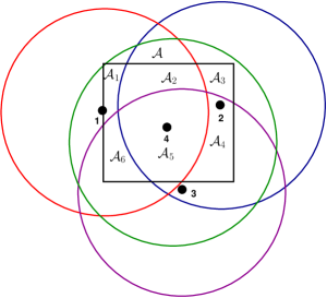
Figure 1: Partitioning of $\mathcal{A}$ in a large $\mathsf{WSN}$ by detection regions: (a simple example) The coloured solid circles around each sensor node denote their detection regions. The four sensor nodes divide the $\mathsf{ROI}$, indicated by the square region, into regions $\mathcal{A}_{1},\cdots,\mathcal{A}_{6}$ such that region $\mathcal{A}_{i}$ is detection–covered by a unique set of sensors $\mathcal{N}_{i}$. For example, ${\cal A}_{1}$ is detection covered by the set of sensors ${\cal N}_{1}=\{1,2,4\}$, etc.

We say that a location $x\in\mathsf{ROI}$ is detection–covered by sensor node $s$, if $\|\ell^{(s)}-x\|\leqslant r_{d}$. For any sensor node $s$, $\mathcal{D}^{(s)}:=\{x\in\mathcal{A}:\|\ell^{(s)}-x\|\leqslant r_{d}\}$ is called its detection–coverage region (see Fig. 1). We assume that the sensor deployment is such that every $x\in\mathcal{A}$ is detection–covered by at least one sensor (Fig. 1). For each $x\in\mathcal{A}$, define $\mathcal{N}(x)$ to be the largest set of sensors by which $x$ is detection–covered, i.e., $\mathcal{N}(x):=\{s:x\in{\cal D}^{(s)}\}$. Let $\mathcal{C}(\mathcal{N})=\{\mathcal{N}(x):x\in{\cal A}\}$. $\mathcal{C}(\mathcal{N})$ is a finite set and can have at most $2^{n}-1$ elements. Let $N=|\mathcal{C}(\mathcal{N})|$. For each $\mathcal{N}_{i}\in\mathcal{C}(\mathcal{N})$, we denote the corresponding detection–covered region by $\mathcal{A}_{i}=\mathcal{A}(\mathcal{N}_{i}):=\{x\in\mathsf{ROI}:\mathcal{N}(x)=\mathcal{N}_{i}\}$. Evidently, the ${\cal A}_{i},1\leqslant i\leqslant N$, partition the $\mathsf{ROI}$. We say that the $\mathsf{ROI}$ is detection–partitioned into a minimum number of subregions, $\mathcal{A}_{1},\mathcal{A}_{2},\cdots,\mathcal{A}_{N}$, such that the subregion $\mathcal{A}_{i}$ is detection–covered by a unique set of sensors $\mathcal{N}_{i}$, and $\mathcal{A}_{i}$ is the maximal detection–covered region of $\mathcal{N}_{i}$, i.e., $\forall i\neq i^{\prime}$, $\mathcal{N}_{i}\neq\mathcal{N}_{i^{\prime}}$ and $\mathcal{A}_{i}\cap\mathcal{A}_{i^{\prime}}=\emptyset$. See Fig. 1 for an example.

II-C Sensor Measurement Model

Before change, i.e., for $k<T$, the observation $X_{k}^{(s)}$ at the sensor $s$ is just the zero mean sensor noise $W_{k}^{(s)}$, the probability density function (pdf) of which is denoted by $f_{0}(\cdot)$ (pre–change pdf). After change, i.e., for $k\geqslant T$ with the location of the event being $\ell_{e}$, the observation of sensor $s$ is given by $X_{k}^{(s)}=h_{e}\rho(d_{e,s})+W_{k}^{(s)}$ where $d_{e,s}:=\|\ell^{(s)}-\ell_{e}\|$, the pdf of which is denoted by $f_{1}(\cdot;d_{e,s})$ (post–change pdf). The noise processes $\{W_{k}^{(s)}\}$ are independent and identically distributed (iid) across time and across sensor nodes. In the rest of the paper, we consider $f_{0}(\cdot)$ to be Gaussian with mean 0 and variance $\sigma^{2}$.

We denote the probability measure when the change happens at time $T$ and at location $\ell_{e}$ by ${\sf P}^{({\bf d}(\ell_{e}))}_{T}\left\{\cdot\right\}$, where ${\bf d}(\ell_{e})=[d_{e,1},d_{e,2},\cdots,d_{e,n}]$, and the corresponding expectation operator by ${\sf E}^{({\bf d}(\ell_{e}))}_{T}\left[\cdot\right]$. In the case of Boolean sensing model, the post–change pdfs depend only on the detection subregion where the event occurs, and hence, we denote the probability measure when the event occurs at $\ell_{e}\in{\cal A}_{i}$ and at time $T$ by ${\sf P}^{(i)}_{T}\left\{\cdot\right\}$, and the corresponding expectation operator by ${\sf E}^{(i)}_{T}\left[\cdot\right]$.

II-D Local Change Detectors

We compute a $\mathsf{CUSUM}$ statistic $C_{k}^{(s)},k\geqslant 1$ at each sensor $s$ based only on its own observations. The $\mathsf{CUSUM}$ procedure was proposed by Page [5] as a solution to the classical change detection problem (${\sf CDP}$, in which there is one pre–change hypothesis and only one post–change hypothesis). The optimality of $\mathsf{CUSUM}$ was shown for conditionally iid observations by Moustakides in [18] for a maximum mean delay metric introduced by Pollak [19] which is $\mathsf{SADD}(\tau):=$ $\underset{T\geqslant 1}{\sup}\ \ {\mathsf{E}}_{T}\left[\tau-T|\tau\geqslant T\right]$.

The driving term of $\mathsf{CUSUM}$ should be the log likelihood–ratio (LLR) of $X_{k}^{(s)}$ defined as $Z^{(s)}_{k}(d_{e,s}):=\ln\left(\frac{f_{1}(X_{k}^{(s)};d_{e,s})}{f_{0}(X_{k}^{(s)})}\right)$. As the location of the event $\ell_{e}$ is unknown, the distance $d_{e,s}$ is also unknown. Hence, one cannot work with the pdfs $f_{1}(\cdot;d_{e,s})$. We propose to drive the $\mathsf{CUSUM}$ at each node $s$ with $Z^{(s)}_{k}(r_{d})$, where we recall that $r_{d}$ is the detection range of a sensor. Based on the $\mathsf{CUSUM}$ statistic $C_{k}^{(s)},k\geqslant 1$, sensor $s$ computes a sequence of local decisions $D_{k}^{(s)}\in\{0,1\},k\geqslant 1$, where 0 represents no–change and 1 represents change. For each set of sensor nodes ${\cal N}_{i}$ that detection partitions the $\mathsf{ROI}$, we define $\tau^{({\cal N}_{i})}$, the stopping time (based on the sequence of local decisions $D_{k}^{(s)}$s for all $s\in{\cal N}_{i}$) at which the set of sensors ${\cal N}_{i}$ detects the event. The way we obtain the local decisions $D_{k}^{(s)}$ from the $\mathsf{CUSUM}$ statistic $C_{k}^{(s)},k\geqslant 1$, and the way these local decisions determine the stopping times $\tau^{({\cal N}_{i})}$, varies from rule to rule. Specific rules for local decision and the fusion of local decisions will be described in Section IV (also see [20]).

An implementation strategy for our distributed event detection/isolation procedure can be the following. We assume that the sensors know to which detection sensor sets ${\cal N}_{i}$s they belong. This could be done by initial configuration or by self–organisation. When the local decision of sensor $s$ is 1, it broadcasts this fact to all sensors in its detection neighbourhood. In practise, the broadcast range of these radios is substantially larger than the detection range. Hence, the local decision of $s$ is learnt by all sensors $s^{\prime}$ that belong to ${\cal N}_{i}$ to which $s$ belongs. When any node learns that all the sensors in ${\cal N}_{i}$ have reached the local decision 1, it transmits an alarm message to the base station [21]. A distributed leader election algorithm can be implemented so that only one, or a controlled number of alarms is sent. This alarm message is carried by geographical forwarding [22]. A system that utilises such local fusion (but with a different sensing and detection model) was developed by us and is reported in [23].

II-E Influence Region

After a set of nodes ${\cal N}_{i}$ declares an event, the event is isolated to a region associated with ${\cal N}_{i}$ called the influence region. In the Boolean sensing model, if an event occurs in ${\cal A}_{i}$, then only the sensors $s\in{\cal N}_{i}$ observe the event, while the other sensors ${s^{\prime}\notin{\cal N}_{i}}$ only observe noise. On the other hand, in the power law path–loss model, sensors ${s^{\prime}\notin{\cal N}_{i}}$ can also observe the event, and the driving term of the $\mathsf{CUSUM}$s of sensors $s^{\prime}$ may be affected by the event. The mean of the driving term of $\mathsf{CUSUM}$ of any sensor $s$ is given by

$${\mathsf{E}}_{f_{1}(\cdot;d_{e,s})}[Z_{k}^{(s)}(r_{d})] = \frac{(h_{e}\rho(r_{d}))^{2}}{2\sigma^{2}}\left(\frac{2\rho(d_{e,s})}{\rho(r_{d})}-1\right).$$ (2)

Thus, the mean of the increment that drives $\mathsf{CUSUM}$ of node $s$ decreases with $d_{e,s}$ and becomes negative when $2\rho(d_{e,s})<\rho(r_{d})$. In this region, we are interested in finding $T_{E}$, the expected time for the $\mathsf{CUSUM}$ statistic $C_{k}^{(s)}$ to cross the threshold $c$. Define $\tau^{(s)}:=\inf\left\{k:C_{k}^{(s)}\geqslant c\right\}$, and hence, $T_{E}={\sf E}_{1}^{({\bf d}(\ell_{e}))}\left[\tau^{(s)}\right]$.

Lemma 1

If the distance between sensor node $s$ and the event, $d_{e,s}$ is such that $2\rho(d_{e,s})<\rho(r_{d})$, then

$$T_{E} \geqslant \exp(\omega_{0}c)$$

where $\omega_{0}=1-\frac{2\rho(d)}{\rho(r_{d})}$.

Proof 1

From (Eqn. 5.2.79 pg. 177 of) [24], we can show that ${\sf E}_{1}^{({\bf d}(\ell_{e}))}\left[\tau^{(s)}\right]\geqslant\exp(\omega_{0}c)$ where $\omega_{0}$ is the solution to the equation

$${\sf E}_{1}^{({\bf d}(\ell_{e}))}\left[e^{\omega_{0}Z_{k}^{(i)}(r_{d})}\right]=0,$$

which is given by $\omega_{0}=1-\frac{2\rho(d)}{\rho(r_{d})}$ (see Eqn. (2)).

We would be interested in ${\sf T_{E}}\geqslant\exp(\underline{\omega}_{0}\cdot c)$ for some $0<\underline{\omega}_{0}<1$. We now define the influence range of a sensor as follows.

Definition 2

Influence Range of a sensor, $r_{i}$, is defined as the distance from the sensor within which the occurrence of an event can be detected within a mean delay of $\exp{(\underline{\omega}_{0}c)}$ where $\underline{\omega}_{0}$ is a parameter of interest and $c$ is the threshold of the local $\mathsf{CUSUM}$ detector. Using Lemma 1, we see that $r_{i}=\min\{d^{\prime}:2\rho(d^{\prime})\leqslant(1-\underline{\omega}_{0})\rho(r_{d})\}$. ∎

A location $x\in{\cal A}$ is influence covered by a sensor $s$ if $\|\ell^{(s)}-x\|\leqslant r_{i}$, and a set of sensors ${\cal N}_{j}$ is said to influence cover $x$ if each sensor $s\in{\cal N}_{j}$ influence covers $x$.

From Lemma 1, we see that by having a large value of $\underline{\omega}_{0}$, i.e., $\underline{\omega}_{0}$ close to 1, the sensors that are beyond a distance of $r_{i}$ from the event take a long time to cross the threshold. However, we see from the definition of influence range that a large value of $\underline{\omega}_{0}$ gives a large influence range $r_{i}$. We will see from the discussion in Section II-F that a large influence range results in the isolation of the event to a large subregion of ${\cal A}$. On the other hand, from Section IV-E, we will see that a large $\underline{\omega}_{0}$ decreases the probability of false isolation, a performance metric of change detection/isolation procedure, which we define in Section III.

We define the influence–region of sensor $s$ as $\mathcal{T}^{(s)}\ :=\ \{x\in\mathcal{A}:\|\ell^{(s)}-x\|\leqslant r_{i}\}$. For the Boolean sensing model, $r_{i}=r_{d}$, and hence, ${\cal D}^{(s)}={\cal T}^{(s)}$ for all $1\leqslant s\leqslant n$, and for the power law path–loss sensing model, $r_{i}>r_{d}$, and hence, ${\cal D}^{(s)}\subset{\cal T}^{(s)}$ for all $1\leqslant s\leqslant n$ (see Fig. 2).

(a) Detection and influence regions of the Boolean model

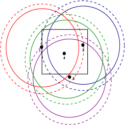
(b) Detection and influence regions of the power law path loss model

Figure 2: Influence and detection regions: A simple example of partitioning of $\mathcal{A}$ in a large $\mathsf{WSN}$. The coloured solid circles around each sensor node denote their detection regions. The four sensor nodes, in the figure, divide the $\mathsf{ROI}$, indicated by the square region, into regions $\mathcal{A}_{1},\cdots,\mathcal{A}_{6}$ such that region $\mathcal{A}_{i}$ is detection–covered by a unique set of sensors $\mathcal{N}_{i}$. The dashed circles represent the influence regions. In the Boolean model, the influence region of a sensor coincides with its detection region.

Recalling the sets of sensors ${\cal N}_{i}$, $1\leqslant i\leqslant N$, defined in Section II-B, we define the influence region of the set of sensors $\mathcal{N}_{i}$ as the region $\mathcal{B}_{i}$ such that each $x\in\mathcal{B}_{i}$ is within the influence range of all the sensors in $\mathcal{N}_{i}$, i.e., $\mathcal{B}_{i}\ :=\ {\cal B}({\cal N}_{i})\ :=\bigcap_{s\in\mathcal{N}_{i}}\mathcal{T}^{(s)}$. Note that $\mathcal{A}(\mathcal{N}_{i})=\left(\underset{s\in\mathcal{N}_{i}}{\bigcap}\mathcal{D}^{(s)}\right)\bigcap\left(\underset{s^{\prime}\notin\mathcal{N}_{i}}{\bigcap}\overline{\mathcal{D}^{(s^{\prime})}}\right)$, where $\overline{{\cal D}}$ is the complement of the set ${\cal D}$, and ${\cal D}^{(s)}\subseteq{\cal T}^{(s)}$. Hence, $\mathcal{A}(\mathcal{N}_{i})\subseteq\mathcal{B}(\mathcal{N}_{i})$. For the power law path–loss sensing model, ${\cal D}^{(s)}\subset{\cal T}^{(s)}$ for all $1\leqslant s\leqslant n$, and hence, $\mathcal{A}(\mathcal{N}_{i})\subset\mathcal{B}(\mathcal{N}_{i})$ for all $1\leqslant i\leqslant N$. For the Boolean sensing model, $\mathcal{A}(\mathcal{N}_{i})=\mathcal{B}(\mathcal{N}_{i})\bigcap\left(\underset{s^{\prime}\notin\mathcal{N}_{i}}{\bigcap}\overline{\mathcal{D}^{(s^{\prime})}}\right)$, and hence $\mathcal{A}(\mathcal{N}_{i})=\mathcal{B}(\mathcal{N}_{i})$ only when ${\cal N}_{i}=\{1,2,\cdots,n\}$. Thus, for a general sensing model, $\mathcal{A}(\mathcal{N}_{i})\subseteq\mathcal{B}(\mathcal{N}_{i})$. We note here that in the Boolean and the power law path loss models, an event which does not lie in the detection subregion of ${\cal N}_{i}$, but lies in its influence subregion (i.e., $\ell_{e}\in\mathcal{B}(\mathcal{N}_{i})\setminus\mathcal{A}(\mathcal{N}_{i})$) can be detected due to ${\cal N}_{i}$ because of the stochastic nature of the observations; in the power law path loss sensing model, this is also because of the difference in losses $\rho(d_{e,s})$ between different sensors.

Remark: The definition of the detection and influence ranges have involved two design parameters $\mu_{1}$ and $\underline{\omega}_{0}$ which can be used to “tune” the performance of the distributed detection schemes that we develop.

∎

II-F Isolating the Event

In Section II D, we provided an outline of a class of distributed detection procedures that will yield a stopping rule. On stopping, a decision for the location of the event is made, which is called isolation. In Section IV, we will provide specific distributed detection/isolation procedures in which stopping will be due to one of the sensor sets ${\cal N}_{i}$.

An event occurring at location $\ell_{e}\in{\cal A}_{i}$ can influence sensors $s^{\prime}$ which influence cover $\ell_{e}$, and hence, the detection can be due to sensors ${\cal N}_{i}\neq{\cal N}_{j}$ which influence cover $\ell_{e}$. Thus, we isolate the event to the influence region of the sensors that detect the event. Because of noise, detection can be due to a sensor set ${\cal N}_{h}$ which does not influence cover the event. Such an error event is called false isolation.

An event occurring at $\ell_{e}\in{\cal A}_{i}$ is influence covered by sensors $s^{\prime}\in{\cal N}(\ell_{e}):=\{s:\|\ell^{(s)}-\ell_{e}\|\leqslant r_{i}\}$. Hence, the detection due to any ${\cal N}_{j}\subseteq{\cal N}(\ell_{e})$ corresponds to the isolation of the event, and that due to ${\cal N}_{j}\not\subseteq{\cal N}(\ell_{e})$ corresponds to false isolation. Note that in the case of Boolean sensing model ${\cal N}(\ell_{e})={\cal N}_{i}$.

In Section III, we formulate the problem of quickest detection of an event and isolating the event to one of the influence subregions $\mathcal{B}_{1},\mathcal{B}_{2},\cdots,\mathcal{B}_{N}$ under a false alarm and false isolation constraint.

III Problem Formulation

We are interested in studying the problem of distributed event detection/isolation in the setting developed in Section II. Given a sample node deployment (i.e., given ${\bm{\ell}}$), and having chosen a value of the detection range, $r_{d}$, we partition the $\mathsf{ROI}$, $\mathcal{A}$ into the detection–subregions, $\mathcal{A}_{1},\mathcal{A}_{2},\cdots,\mathcal{A}_{N}$. Let $\mathcal{N}_{i}$ be the set of sensors that detection–cover the region $\mathcal{A}_{i}$. Having chosen the influence range $r_{i}$, the influence region $\mathcal{B}_{i}$ of the set of sensor nodes $\mathcal{N}_{i}$ can be obtained. We define the following set of hypotheses

$${\bf H}_{0} : \text{event not occurred},$$

$${\bf H}_{T,i} : \text{event occurred at time $T$ in subregion}\ \mathcal{A}_{i},\ \ T=1,2,\cdots,\ i=1,2,\cdots,N.$$

The event occurs in one of the detection subregions ${\cal A}_{i}$, but we will only be able to isolate it to one of the influence subregions ${\cal B}_{i}$ that is consistent with the ${\cal A}_{i}$ (see Section II-F). We study distributed procedures described by a stopping time $\tau$, and an isolation decision $L(\tau)\in\{1,2,\cdots,N\}$ (i.e., the tuple $(\tau,L)$) that detect an event at time $\tau$ and locate it to $L(\tau)$ (i.e., to the influence region $\mathcal{B}_{L(\tau)}$) subject to a false alarm and false isolation constraint. The false alarm constraint considered is the average run length to false alarm $\mathsf{ARL2FA}$, and the false isolation constraint considered is the probability of false isolation $\mathsf{PFI}$, each of which we define as follows.

Definition 3

The Average Run Length to False Alarm $\mathsf{ARL2FA}$ of a change detection/isolation procedure $\tau$ is defined as the expected number of samples taken under null hypothesis ${\bf H}_{0}$ to raise an alarm, i.e.,

$$\mathsf{ARL2FA}(\tau) := {\sf E}_{\infty}\left[\tau\right],$$

where ${\sf E}_{\infty}[\cdot]$ is the expectation operator (with the corresponding probability measure being ${\sf P}_{\infty}\{\}$) when the change occurs at infinity. ∎

Definition 4

The Probability of False Isolation $\mathsf{PFI}$ of a change detection/isolation procedure $\tau$ is defined as the supremum of the probabilities of making an incorrect isolation decision, i.e.,

$$\mathsf{PFI}(\tau)\ :=\ \max_{1\leqslant i\leqslant N}\ \sup_{\ell_{e}\in{\cal A}_{i}}\ \max_{1\leqslant j\leqslant N,{\cal N}_{j}\not\subseteq{\cal N}(\ell_{e})}\ {\mathsf{P}}_{1}^{({\bf d}(\ell_{e}))}\left\{L(\tau)=j\right\}$$

where we recall that ${\cal N}(\ell_{e})=\{s:\|\ell^{(s)}-\ell_{e}\|\leqslant r_{i}\}$ is the set of sensors that influence covers $\ell_{e}\in{\cal A}_{i}$. ∎

In the case of Boolean sensing model, the post–change pdfs depend only on the index $i$ of the detection subregion where the event occurs, and hence, the $\mathsf{PFI}$ is given by

$$\mathsf{PFI}(\tau)\ :=\ \max_{1\leqslant i\leqslant N}\ \max_{1\leqslant j\leqslant N,{\cal N}_{j}\not\subseteq{\cal N}_{i}}\ {\mathsf{P}}_{1}^{(i)}\left\{L(\tau)=j\right\}.$$

In [2], Nikiforov defined the probability of false isolation, also, over the set of all possible change times, as ${\sf SPFI}(\tau)\ :=\ \sup_{1\leqslant i\leqslant N}\ \ \sup_{1\leqslant j\neq i\leqslant N}\ \ \sup_{T\geqslant 1}\ {\mathsf{P}}_{T}^{(i)}\left\{L(\tau)=j\mid\tau\geqslant T\right\}$. Define the following classes of change detection/isolation procedures,

$${\Delta}(\gamma,\alpha) := \left\{(\tau,L):\mathsf{ARL2FA}(\tau)\geqslant\gamma,{\sf SPFI}(\tau)\leqslant\alpha\right\},$$

$$\widetilde{\Delta}(\gamma,\alpha) := \left\{(\tau,L):\mathsf{ARL2FA}(\tau)\geqslant\gamma,\mathsf{PFI}(\tau)\leqslant\alpha\right\}.$$

We define the supremum average detection delay $\mathsf{SADD}$ performance for the procedure $\tau$, in the same sense as Pollak [19] (also see [2]), as the maximum mean number of samples taken under any hypothesis ${\bf H}_{T,i},\ i=1,2,\cdots,N$, to raise an alarm, i.e.,

$$\mathsf{SADD}(\tau):=\underset{\ell_{e}\in\mathcal{A}}{\sup}\ \underset{T\geqslant 1}{\sup}\ {\mathsf{E}}^{({\bf d}({\ell_{e}}))}_{T}\left[\tau-T|\tau\geqslant T\right].$$

We are interested in obtaining an optimal procedure $\tau$ that minimises the $\mathsf{SADD}$ subject to the average run length to false alarm and the probability of false isolation constraints,

$$\inf \underset{\ell_{e}\in\mathcal{A}}{\sup}\ \underset{T\geqslant 1}{\sup}\ {\mathsf{E}}^{({\bf d}(\ell_{e}))}_{T}\left[\tau-T|\tau\geqslant T\right]$$

subject to $$\begin{array}[]{rcl}\mathsf{ARL2FA}(\tau)&\geqslant&\gamma\\ \mathsf{PFI}(\tau)&\leqslant&\alpha.\end{array}$$

The change detection/isolation problem that we pose here is motivated by the framework of [1], [2], [3], which we discuss in the next subsection.

III-A Centralised Recursive Solution for the Boolean Sensing Model

In [2], Nikiforov and in [3], Tartakovsky studied a change detection/isolation problem that involves $N>1$ post–change hypotheses (and one pre–change hypothesis). Thus, their formulation can be applied to our problem. But, in their model, the pdf of ${\bf X}_{k}$ for $k\geqslant T$, under hypothesis ${\bf H}_{T,i}$, $g_{i}$ is completely known. It should be noted that in our problem, in the case of power law path–loss sensing model, the pdf of the observations under any post–change hypothesis is unknown as the location of the event is unknown. The problem posed by Nikiforov [2] is

$$\inf_{(\tau,L)\in{\Delta}(\gamma,\alpha)} \underset{1\leqslant i\leqslant N}{\sup}\ \sup{\mathsf{E}}^{(i)}_{T}\left[\tau-T|\tau\geqslant T\right],$$ (4)

and that by Tartakovsky [3] is

$$\inf_{(\tau,L)\in\widetilde{\Delta}(\gamma,\alpha)} \underset{1\leqslant i\leqslant N}{\sup}\ \sup{\mathsf{E}}^{(i)}_{T}\left[\tau-T|\tau\geqslant T\right].$$ (5)

Nikiforov [2] and Tartakovsky [3] obtained asymptotically optimal centralised change detection/isolation procedures as $\min\{\gamma,\frac{1}{\alpha}\}\to\infty$, the $\mathsf{SADD}$ of which is given by the following theorem.

Theorem 1 (Nikiforov 03)

For the $N$–hypotheses change detection/isolation problem (for the Boolean sensing model) defined in Eqn. (4), the asymptotically maximum mean delay optimal detection/isolation procedure $\tau^{\sf*}$ has the property,

$$\mathsf{SADD}(\tau^{\sf*}) \stackrel{{\scriptstyle\leqslant}}{{\sim}} \max\left\{\frac{\ln\gamma}{\underset{1\leqslant i\leqslant N}{\min}\ \ \ \mbox{KL}(g_{i},g_{0})},\frac{-\ln(\alpha)}{\underset{1\leqslant i\leqslant N,1\leqslant j\neq i\leqslant N}{\min}\ \ \mbox{KL}(g_{i},g_{j})}\right\},\ \ \text{as}\ \min\left\{\gamma,\frac{1}{\alpha}\right\}\to\infty,$$

where $\mbox{KL}(\cdot,\cdot)$ is the Kullback–Leibler divergence function, and $g_{i}$ is the pdf of the observation ${\bf X}_{k}$ for $k\geqslant T$ under hypothesis ${\bf H}_{T,i}$. ∎

Remark: Since, ${\Delta}(\gamma,\alpha)\subseteq\widetilde{\Delta}(\gamma,\alpha)$, the asymptotic upper bound on $\mathsf{SADD}$ for $\tau^{*}$ is also an upper bound for the $\mathsf{SADD}$ over the set of procedures in $\widetilde{\Delta}(\gamma,\alpha)$.

In the case of Boolean sensing model, for any post–change hypothesis ${\bf H}_{T,i}$, only the set of sensor nodes that detection cover (which is the same as influence cover) the subregion ${\cal A}_{i}$ switch to a post–change pdf $f_{1}$ (and the distribution of other sensor nodes continues to be $f_{0}$). Since the pdf of the sensor observations are conditionally i.i.d., the pdf of the observation vector, in the Boolean sensing model, corresponds to the post–change pdf $g_{i}$ of the centralised problem studied by Nikiforov [2] and by Tartakovsky [3]. Thus, their problem directly applies to our setting with the Boolean sensing model. In our work, however, we propose algorithms for the change detection/isolation problem for the power law sensing model as well. Also, the procedures proposed by Nikiforov and by Tartakovsky are (while being recursive) centralised, whereas we propose distributed procedures which are computationally simple.

In Section IV, we propose distributed detection/isolation procedures $\sf{MAX}$, $\sf{HALL}$ and $\sf{ALL}$ and analyse their false alarm ($\mathsf{ARL2FA}$), false isolation ($\mathsf{PFI}$) and the detection delay ($\mathsf{SADD}$) properties.

IV Distributed Change Detection/Isolation Procedures

In this section, we study the procedures $\sf{MAX}$ and $\sf{ALL}$ for change detection/isolation in a distributed setting. Also, we propose a distributed detection procedure “${\sf HALL}$,” and analyse the $\mathsf{SADD}$, the $\mathsf{ARL2FA}$, and the $\mathsf{PFI}$ performance.

IV-A The $\sf{MAX}$ Procedure

Tartakovsky and Veeravalli proposed a decentralised procedure $\sf{MAX}$ for a collocated scenario in [6]. We extend the $\sf{MAX}$ procedure to a large $\mathsf{WSN}$ under the $\mathsf{ARL2FA}$ and $\mathsf{PFI}$ constraints. Recalling Section II, each sensor node $i$ employs $\mathsf{CUSUM}$ for local change detection between pdfs $f_{0}$ and $f_{1}(\cdot;r_{d})$. Let $\tau^{(i)}$ be the random time at which the $\mathsf{CUSUM}$ statistic of sensor node $i$ crosses the threshold $c$ for the first time. At each time $k$, the local decision of sensor node $i$, $D_{k}^{(i)}$ is defined as

$$D_{k}^{(i)} := \left\{\begin{array}[]{ll}0,&\text{for}\ k<\tau^{(i)}\\ 1,&\text{for}\ k\geqslant\tau^{(i)}.\end{array}\right.$$

The global decision rule $\tau^{\sf{MAX}}$ declares an alarm at the earliest time slot $k$ at which all sensor nodes $j\in\mathcal{N}_{i}$ for some $i=1,2,\cdots,N$ have crossed the threshold $c$. Thus,

$$\tau^{\mathsf{MAX},(\mathcal{N}_{i})} := \inf\left\{k:D_{k}^{(j)}=1,\ \forall j\in\mathcal{N}_{i}\right\}\ =\ \min\left\{\tau^{(j)}:j\in\mathcal{N}_{i}\right\}$$

$$\tau^{\mathsf{MAX}} := \min\left\{\tau^{\mathsf{MAX},(\mathcal{N}_{i})}:1\leqslant i\leqslant N\right\}.$$

i.e., the MAX procedure declares an alarm at the earliest time instant when the $\mathsf{CUSUM}$ statistic of all the sensor nodes ${\cal N}_{i}$ corresponding to hypothesis ${\bf H}_{T,i}$ of some $i$ have crossed the threshold at least once. The isolation rule is $L(\tau)=\arg\min_{1\leqslant i\leqslant N}\{\tau^{\sf MAX,({\cal N}_{i})}\}$, i.e., to declare that the event has occurred in the influence region ${\cal B}_{L(\tau)}=\mathcal{B}(\mathcal{N}_{L(\tau)})$ corresponding to the set of sensors $\mathcal{N}_{L(\tau)}$ that raised the alarm.

IV-B $\sf{ALL}$ Procedure

Mei, [9], and Tartakovsky and Kim, [25], proposed a decentralised procedure $\sf{ALL}$, again for a collocated network. We extend the $\sf{ALL}$ procedure to a large extent network under the $\mathsf{ARL2FA}$ and the $\mathsf{PFI}$ constraints. Here, each sensor node $i$ employs $\mathsf{CUSUM}$ for local change detection between pdfs $f_{0}$ and $f_{1}(\cdot;r_{d})$. Let $C_{k}^{(i)}$ be the $\mathsf{CUSUM}$ statistic of sensor node $i$ at time $k$. The $\mathsf{CUSUM}$ in the sensor nodes is allowed to run freely even after crossing the threshold $c$. Here, the local decision of sensor node $i$ is

$$D_{k}^{(i)} := \left\{\begin{array}[]{ll}0,&\text{if}\ C_{k}^{(i)}<c\\ 1,&\text{if}\ C_{k}^{(i)}\geqslant c.\end{array}\right.$$

The global decision rule $\tau^{\sf{ALL}}$ declares an alarm at the earliest time slot $k$ at which the local decision of all the sensor nodes corresponding to a set $\mathcal{N}_{i}$, for some $i=1,2,\cdots,N$, are 1, i.e.,

$$\tau^{\mathsf{ALL},(\mathcal{N}_{i})} := \inf\left\{k:D_{k}^{(j)}=1,\ \forall j\in\mathcal{N}_{i}\right\}\ =\ \inf\left\{k:C_{k}^{(j)}\geqslant c,\forall j\in\mathcal{N}_{i}\right\}$$

$$\tau^{\mathsf{ALL}} := \min\left\{\tau^{\mathsf{ALL},(\mathcal{N}_{i})}:1\leqslant i\leqslant N\right\}.$$

The isolation rule is $L(\tau)\ =\ \arg\min_{1\leqslant i\leqslant N}\{\tau^{\sf ALL,({\cal N}_{i})}\}$, i.e., to declare that the event has occurred in the influence region ${\cal B}_{L(\tau)}=\mathcal{B}(\mathcal{N}_{L(\tau)})$ corresponding to the set of sensors $\mathcal{N}_{L(\tau)}$ that raised the alarm.

IV-C $\sf{HALL}$ Procedure

Figure 3: ALL and HALL: Evolution of $\mathsf{CUSUM}$ statistic $C_{k}^{(i)}$ of node $i$ plotted vs. $k$. Note that at time $k=V_{j}^{(i)}$, $R_{j}^{(i)}$ is the excess above the threshold.

Motivated by ${\sf ALL}$, and the fact that sensor noise can make the $\mathsf{CUSUM}$ statistic fluctuate around the threshold, we propose a local decision rule which is 0 when the $\mathsf{CUSUM}$ statistic has visited zero and has not crossed the threshold yet and is 1 otherwise. We explain the $\sf{HALL}$ procedure below.

The following discussion is illustrated in Fig. 3. Each sensor node $i$ computes a $\mathsf{CUSUM}$ statistic $C_{k}^{(i)}$ based on the LLR of its own observations between the pdfs $f_{1}(\cdot;r_{d})$ and $f_{0}$. Define $U_{0}^{(i)}:=0$. Define $V_{1}^{(i)}$ as the time at which $C_{k}^{(i)}$ crosses the threshold $c$ (for the first time) as:

$$V_{1}^{(i)}:=\inf\left\{k:C_{k}^{(i)}\geqslant c\right\}$$

(see Fig. 3 where the “overshoots” $R_{k}^{(i)}$, at $V_{k}^{(i)}$, are also shown). Note that $\inf\emptyset:=\infty$. Next define

$$U_{1}^{(i)}:=\inf\left\{k>V_{1}^{(i)}:C_{k}^{(i)}=0\right\}.$$

Now starting with $U_{1}^{(i)}$, we can recursively define $V_{2}^{(i)},U_{2}^{(i)}$ etc. in the obvious manner (see Fig. 3). Each node $i$ computes the local decision $D_{k}^{(i)}$ based on the $\mathsf{CUSUM}$ statistic $C_{k}^{(i)}$ as follows:

$$D_{k}^{(i)} = \left\{\begin{array}[]{lll}1,&\text{if}\ V^{(i)}_{j}\leqslant k<U^{(i)}_{j}\ \text{ for some }j\\ 0,&\text{otherwise.}\end{array}\right.$$ (10)

The global decision rule is a stopping time $\tau^{\sf{HALL}}$ defined as the earliest time slot $k$ at which all the sensor nodes in a region have a local decision $1$, i.e.,

$$\tau^{\mathsf{HALL},(\mathcal{N}_{i})} := \inf\left\{k:D_{k}^{(j)}=1,\ \forall j\in\mathcal{N}_{i}\right\},$$

$$\tau^{\mathsf{HALL}} := \min\left\{\tau^{\mathsf{HALL},(\mathcal{N}_{i})}:1\leqslant i\leqslant N\right\}.$$

The isolation rule is $L(\tau)=\arg\min_{1\leqslant i\leqslant N}\{\tau^{\sf HALL,({\cal N}_{i})}\}$, i.e., to declare that the event has occurred in the influence region ${\cal B}_{L(\tau)}=\mathcal{B}(\mathcal{N}_{L(\tau)})$ corresponding to the set of sensors $\mathcal{N}_{L(\tau)}$ that raised the alarm.

Remark: The procedures $\sf{HALL},\sf{MAX}$ and $\sf{ALL}$ differ only in their local decision rule; the global decision rule as a function of $\{D_{k}^{(i)}\}$ is the same for $\sf{HALL},\sf{MAX}$ and $\sf{ALL}$. For the distributed procedures $\sf{MAX}$, $\sf{ALL}$, and $\sf{HALL}$, we analyse the $\mathsf{ARL2FA}$ in Section IV-D, the $\mathsf{PFI}$ in Section IV-E, and the $\mathsf{SADD}$ performance in Section IV-F.

IV-D Average Run Length to False Alarm ($\mathsf{ARL2FA}$)

From the previous sections, we see that the stopping time of any ${\sf procedure}$ ($\mathsf{MAX}$, $\mathsf{ALL}$, or ${\sf HALL}$) is the minimum of the stopping times corresponding to each ${\cal N}_{i}$, i.e.,

$$\tau^{\mathsf{procedure}} := \min\left\{\tau^{\mathsf{procedure},(\mathcal{N}_{i})}:1\leqslant i\leqslant N\right\}.$$

Under the null hypothesis ${\bf H}_{0}$, the $\mathsf{CUSUM}$ statistics $C_{k}^{(s)}$s of sensors $s\in{\cal N}_{i}$ are driven by independent noise processes, and hence, $C_{k}^{(s)}$s are independent. But, there can be a sensor that is common to two different ${\cal N}_{i}$s, and hence, $\tau^{\mathsf{procedure},(\mathcal{N}_{i})}$s, in general, are not independent. We provide asymptotic lower bounds for the $\mathsf{ARL2FA}$ for $\sf{MAX}$, $\sf{HALL}$, and $\sf{ALL}$, in the following theorem.

Theorem 2

For local $\mathsf{CUSUM}$ threshold $c$,

$$\mathsf{ARL2FA}(\tau^{\sf MAX}) \geqslant \exp\left(a_{\sf MAX}c\right)\cdot(1+o(1))$$ (11)

$$\mathsf{ARL2FA}(\tau^{\sf HALL}) \geqslant \exp\left(a_{\sf HALL}c\right)\cdot(1+o(1))$$ (12)

$$\mathsf{ARL2FA}(\tau^{\sf ALL}) \geqslant \exp\left(a_{\sf ALL}c\right)\cdot(1+o(1))$$ (13)

($o(1)\to 0$ as $c\to\infty$), where for any arbitrarily small $\delta>0$, $a_{\sf MAX}=a_{\sf HALL}=1-\delta$, $a_{\sf ALL}=m-\delta$,

where $m=\min\{{\cal N}_{i}\setminus\bigcup_{\begin{subarray}{c}j\neq i,\ \end{subarray}{j\in{\cal I}}}{\cal N}_{j}:i\in{\cal I}\}$, ${\cal I}$ is the set of indices of the detection sets that are minimal in the partially order of set inclusion among the detection sets.

Proof 2

See Appendix A.

Thus, for ${\sf procedure}$, for a given $\mathsf{ARL2FA}$ requirement of $\gamma$, it is sufficient to choose the threshold $c$ as

$$c =\frac{\ln\gamma}{a_{\sf procedure}}(1+o(1)),\ \ \text{as $\gamma\to\infty$}.$$ (14)

IV-E Probability of False Isolation ($\mathsf{PFI}$)

A false isolation occurs when the hypothesis ${\bf H}_{T,i}$ is true for some $i$ and the hypothesis ${\bf H}_{T,j}\neq{\bf H}_{T,i}$ is declared to be true at the time of alarm, and the event does not lie in the region $\mathcal{B}(\mathcal{N}_{j})$. The following theorem provide asymptotic upper bounds for the $\mathsf{PFI}$ for each of the procedures $\mathsf{MAX}$, $\mathsf{ALL}$, and $\mathsf{HALL}$.

Theorem 3

For local $\mathsf{CUSUM}$ threshold $c$,

$${\sf PFI}(\tau^{\mathsf{MAX}}) \leqslant \frac{\exp\left(-b_{\sf MAX}c\right)}{B_{\sf MAX}}\cdot(1+o(1))$$ (15)

$${\sf PFI}(\tau^{\mathsf{HALL}}) \leqslant \frac{\exp\left(-b_{\sf HALL}c\right)}{B_{\sf HALL}}\cdot(1+o(1))$$ (16)

$${\sf PFI}(\tau^{\mathsf{ALL}}) \leqslant \frac{\exp\left(-b_{\sf ALL}c\right)}{B_{\sf ALL}}\cdot(1+o(1)).$$ (17)

where $o(1)\to 0$ as $c\to\infty$, and $b_{\sf MAX}=b_{\sf HALL}=\frac{m\underline{\xi\omega}_{0}}{2}-\frac{1+\bar{m}}{n}$, $b_{\sf ALL}=\frac{m\underline{\xi\omega}_{0}}{2}-\frac{1}{n}$, $\underline{\omega}_{0}=1$ for Boolean sensing model, $\xi$ is 2 for Boolean sensing model and is 1 for path–loss sensing model, $m=\min\left\{|{\cal N}_{j}\setminus{\cal N}(\ell_{e})|:{1\leqslant i\leqslant N,\ell_{e}\in{\cal A}_{i},1\leqslant j\leqslant N,{\cal N}_{j}\not\subseteq{\cal N}(\ell_{e})}\right\}$ and

$\bar{m}=\max\left\{|{\cal N}_{j}\setminus{\cal N}(\ell_{e})|:{1\leqslant i\leqslant N,\ell_{e}\in{\cal A}_{i},1\leqslant j\leqslant N,{\cal N}_{j}\not\subseteq{\cal N}(\ell_{e})}\right\}$, and $B_{\sf MAX}$, $B_{\sf HALL}$, and $B_{\sf ALL}$ are positive constants.

Proof 3

See Appendix B.

Thus, for a given $\mathsf{PFI}$ requirement of $\alpha$, the threshold $c$ for should satisfy

$$c\ =\ \frac{-\ln B_{\sf procedure}-\ln\alpha}{b_{\sf procedure}}(1+o(1))\ =\ \frac{-\ln\alpha}{b_{\sf procedure}}(1+o(1)),\ \ \ \text{as $\alpha\to 0$}.$$ (18)

IV-F Supremum Average Detection Delay (SADD)

In this section, we analyse the $\mathsf{SADD}$ performance of the distributed detection/isolation procedures. We observe that for any sample path of the observation process, for the same threshold $c$, the ${\mathsf{MAX}}$ rule raises an alarm first, followed by the ${\mathsf{HALL}}$ rule, and then by the ${\mathsf{ALL}}$ rule. This ordering is due to the following reason. For each sensor node $s$, let $\tau^{(s)}$ be the first time instant at which the $\mathsf{CUSUM}$ statistic $C_{k}^{(s)}$ crosses the threshold $c$ (denoted by $V_{1}^{(i)}$ in Figure 3). Before time $\tau^{(s)}$, the local decision is 0 for all the procedures, ${\sf MAX}$, ${\sf ALL}$, and ${\sf HALL}$. For ${\mathsf{MAX}}$, for all $k\geqslant\tau^{(s)}$, the local decision $D_{k}^{(s)}=1$. Thus, the stopping time of $\mathsf{MAX}$ is at least as early as that of ${\mathsf{HALL}}$ and $\mathsf{ALL}$. The local decision of $\mathsf{ALL}$ is 1 ($D_{k}^{(s)}=1$) only at those times $k$ for which $C_{k}^{(s)}\geqslant c$. However, even when $C_{k}^{(s)}<c$, the local decision of $\mathsf{HALL}$ is 1 if $V_{j}^{(s)}\leqslant k<U_{j}^{(s)}$ (see Figure 3) for some $j$. Thus, the local decisions of ${\sf MAX}$, ${\sf HALL}$, and ${\sf ALL}$ are ordered as, for all $k\geqslant 1$, $D_{k}^{(s)}(\mathsf{MAX})\geqslant D_{k}^{(s)}(\mathsf{HALL})\geqslant D_{k}^{(s)}(\mathsf{ALL})$, and hence, $\tau^{\mathsf{MAX},({\cal N}_{i})}\leqslant\tau^{\mathsf{HALL},{(\cal N}_{i})}\leqslant\tau^{\mathsf{ALL},{(\cal N}_{i})}$. Each of the stopping times $\sf{MAX}$, $\sf{HALL}$, or $\sf{ALL}$ is the minimum of stopping times corresponding to the sets of sensors $\{\mathcal{N}_{i}:i=1,2,\cdots,N\}$, i.e.,

$$\tau^{\mathsf{procedure}} = \min\{\tau^{\mathsf{procedure},(\mathcal{N}_{i})}:i=1,2,\cdots,N\}$$

where “$\mathsf{procedure}$” can be $\mathsf{MAX}$ or $\mathsf{HALL}$ or $\mathsf{ALL}$. Hence, we have

$$\tau^{\mathsf{MAX}}\ \leqslant\ \tau^{\mathsf{HALL}}\ \leqslant\ \tau^{\mathsf{ALL}}.$$ (19)

From [9], we see that

$$\sup_{T\geqslant 1}\ {\mathsf{E}}_{T}^{(i)}\left[\tau^{\mathsf{ALL},({\cal N}_{i})}-T\mid\tau^{\sf ALL,({\cal N}_{i})}\geqslant T\right] = \frac{c}{I}\left(1+o(1)\right)$$ (20)

where $I$ is the Kullback–Leibler divergence between the post–change and the pre–change pdfs. For $\ell_{e}\in\mathcal{A}_{i}$, we have $\forall s\in\mathcal{N}_{i},\ d_{e,s}\leqslant r_{d}$. Also, since $\tau^{\mathsf{ALL}}\leqslant\tau^{\mathsf{ALL},({\cal N}_{i})}$, we have

$$\sup_{\ell_{e}\in{\cal A}_{i}}\ \sup_{T\geqslant 1}\ {\mathsf{E}}_{T}^{({\bf d}({\ell_{e}}))}\left[\tau^{\mathsf{ALL}}-T\mid\tau^{\sf ALL}\geqslant T\right] \leqslant \sup_{\ell_{e}\in{\cal A}_{i}}\ \sup_{T\geqslant 1}\ {\mathsf{E}}_{T}^{({\bf d}({\ell_{e}}))}\left[\tau^{\mathsf{ALL},({\cal N}_{i})}-T\mid\tau^{\sf ALL}\geqslant T\right]$$ (21)

From Appendix C, Eqn. (21) becomes,

$$\sup_{\ell_{e}\in{\cal A}_{i}}\ \sup_{T\geqslant 1}\ {\mathsf{E}}_{T}^{({\bf d}({\ell_{e}}))}\left[\tau^{\mathsf{ALL}}-T\mid\tau^{\sf ALL}\geqslant T\right] \leqslant \sup_{\ell_{e}\in{\cal A}_{i}}\ \sup_{T\geqslant 1}\ {\mathsf{E}}_{T}^{({\bf d}({\ell_{e}}))}\left[\tau^{\mathsf{ALL},({\cal N}_{i})}-T\mid\tau^{\sf ALL,({\cal N}_{i})}\geqslant T\right]$$ (22)

$$= \frac{c}{\mathsf{KL}(f_{1}(\cdot;r_{d}),f_{0})}(1+o(1))$$

From the above equation, and from Eqn. (19), we have

$$\mathsf{SADD}(\tau^{\mathsf{MAX}})\ \leqslant\ \mathsf{SADD}(\tau^{\mathsf{HALL}})\ \leqslant\ \mathsf{SADD}(\tau^{\mathsf{ALL}})\ \leqslant\ \frac{c}{\mathsf{KL}(f_{1}(\cdot;r_{d}),f_{0})}(1+o(1)),\ \text{as}\ c\to\infty,$$ (23)

Remark: Recall from Section II-B that $\mu_{1}=h_{e}\rho(r_{d})$. We now see that $\mu_{1}$ governs the detection delay performance, and $\mu_{1}$ can be chosen such that a requirement on $\mathsf{SADD}$ is met. Thus, to achieve a requirement on $\mathsf{SADD}$, we need to choose $r_{d}$ appropriately. A small value of $r_{d}$ (gives a large $\mu_{1}$ and hence,) gives less detection delay compared to a large value of $r_{d}$. But, a small $r_{d}$ requires more sensors to detection–cover the $\mathsf{ROI}$.

In the next subsection, we discuss the asymptotic minimax delay optimality of the distributed procedures in relation to Theorem 1.

IV-G Asymptotic Upper Bound on $\mathsf{SADD}$

For any change detection/isolation procedure to achieve a $\mathsf{ARL2FA}$ requirement of $\gamma$ and $\mathsf{PFI}$ requirement of $\alpha$, a threshold $c$ is chosen such that it satisfies Eqns. 14 and 18, i.e.,

$$c = \max\left\{\frac{\ln\gamma}{a_{\sf procedure}},\frac{-\ln\alpha}{b_{\sf procedure}}\right\}(1+o(1)).$$ (24)

Therefore, from Eqn.(23), the $\mathsf{SADD}$ is given by

$$\mathsf{SADD}(\tau^{\mathsf{procedure}}) \leqslant \frac{1}{\mathsf{KL}(f_{1}(\cdot;r_{d}),f_{0})}\cdot\max\left\{\frac{\ln\gamma}{a_{\sf procedure}},\frac{-\ln\alpha}{b_{\sf procedure}}\right\}(1+o(1)).$$ (25)

where $o(1)\to 0$ as $\min\{\gamma,\frac{1}{\alpha}\}\to\infty$. Note that as $r_{d}$ decreases, $\mathsf{KL}(f_{1}(\cdot;r_{d}),f_{0})=\frac{h_{e}^{2}\rho(r_{d})^{2}}{2\sigma^{2}}$ increases. Thus, to achieve a smaller detection delay, the detection range $r_{d}$ can be decreased, and the number of sensors $n$ can be increased to cover the $\mathsf{ROI}$.

We can compare the asymptotic $\mathsf{SADD}$ performance of the distributed procedures $\sf{HALL}$, $\sf{MAX}$ and $\sf{ALL}$ against Theorem 1 for the Boolean sensing model. For Gaussian pdfs $f_{0}$ and $f_{1}$, the KL divergence between the hypotheses ${\bf H}_{T,i}$ and ${\bf H}_{T,j}$ is given by

$$\mathsf{KL}(g_{i},g_{j}) = \int\ln\left(\frac{\prod_{s\in{\cal N}_{i}}f_{1}(x^{(s)})\prod_{s^{\prime}\notin{\cal N}_{i}}f_{0}(x^{(s^{\prime})})}{{\prod_{s\in{\cal N}_{j}}f_{1}(x^{(s)})\prod_{s^{\prime}\notin{\cal N}_{j}}f_{0}(x^{(s^{\prime})})}}\right)\ \prod_{s\in{\cal N}_{i}}f_{1}(x^{(s)})\prod_{s^{\prime}\notin{\cal N}_{i}}f_{0}(x^{(s^{\prime})})\ d{\bf x}$$

$$= \int\left(\ln\left(\prod_{s\in{\cal N}_{i}}\frac{f_{1}(x^{(s)})}{f_{0}(x^{(s)})}\right)-\ln\left({\prod_{s\in{\cal N}_{j}}\frac{f_{1}(x^{(s)})}{f_{0}(x^{(s)})}}\right)\right)\ \prod_{s\in{\cal N}_{i}}f_{1}(x^{(s)})\prod_{s^{\prime}\notin{\cal N}_{i}}f_{0}(x^{(s^{\prime})})\ d{\bf x}$$

$$= \sum_{s\in{\cal N}_{i}}\mathsf{KL}(f_{1},f_{0})-\sum_{s\in{{\cal N}_{j}\cap\cal N}_{i}}\mathsf{KL}(f_{1},f_{0})+\sum_{s\in{\cal N}_{j}\setminus{\cal N}_{i}}\mathsf{KL}(f_{1},f_{0})$$

$$= |{\cal N}_{i}~{}\Delta~{}{\cal N}_{j}|\ \mathsf{KL}(f_{1},f_{0})$$

where the operator $\Delta$ represents the symmetric difference between the sets. Thus, from Theorem 1 for Gaussian $f_{0}$ and $f_{1}$, we have

$$\mathsf{SADD}(\tau^{*}) \leqslant \frac{1}{\mathsf{KL}(f_{1},f_{0})}\cdot\max\left\{\frac{\ln\gamma}{a^{*}},\frac{-\ln\alpha}{b^{*}}\right\}(1+o(1)),$$

$$\text{where}\ a^{*} = \min_{1\leqslant i\leqslant N}|{\cal N}_{i}|,$$

$$\text{and}\ b^{*} = \min_{\begin{subarray}{c}1\leqslant i\leqslant N\\ 1\leqslant j\leqslant N,\ {\cal N}_{j}\not\subseteq{\cal N}_{i}\end{subarray}}|{\cal N}_{i}\Delta{\cal N}_{j}|.$$

The $\mathsf{SADD}$ performance of the distributed ${\sf procedure}$ with the Boolean sensing model is

$$\mathsf{SADD}(\tau^{\mathsf{procedure}}) \leqslant \frac{1}{\mathsf{KL}(f_{1},f_{0})}\cdot\max\left\{\frac{\ln\gamma}{a_{\sf procedure}},\frac{-\ln\alpha}{b_{\sf procedure}}\right\}(1+o(1)).$$ (26)

where $o(1)\to 0$ as $\min\{\gamma,\frac{1}{\alpha}\}\to\infty$. Thus, the asymptotically optimal upper bound on $\mathsf{SADD}$ (which corresponds to the optimum centralised procedure $\tau^{*}$) and that of the distributed procedures $\mathsf{ALL}$, ${\sf{HALL}}$, and ${\sf{MAX}}$ scale in the same way as $\ln\gamma/\mathsf{KL}(f_{1},f_{0})$ and $-\ln\alpha/\mathsf{KL}(f_{1},f_{0})$.

V Numerical Results

We consider a deployment of 7 nodes with the detection range $r_{d}=1$, in a hexagonal $\mathsf{ROI}$ (see Fig. 4) such that we get $N=12$ detection subregions, and ${\cal N}_{1}=\{1,3,4,6\}$, ${\cal N}_{2}=\{1,3,4\}$, ${\cal N}_{3}=\{1,2,3,4\}$, ${\cal N}_{4}=\{1,2,4\}$, ${\cal N}_{5}=\{1,2,4,5\}$, ${\cal N}_{6}=\{2,4,5\}$, ${\cal N}_{7}=\{2,4,5,7\}$, ${\cal N}_{8}=\{4,5,7\}$, ${\cal N}_{9}=\{4,5,6,7\}$, ${\cal N}_{10}=\{4,6,7\}$, ${\cal N}_{11}=\{3,4,6,7\}$, and ${\cal N}_{12}=\{3,4,6\}$. The pre–change pdf considered is $f_{0}\sim\mathcal{N}(0,1)$, and the detection range and the influence range considered are $r_{d}=1.0$ and $r_{i}=1.5$ respectively.

We compute the $\mathsf{SADD}$, the $\mathsf{ARL2FA}$ and the $\mathsf{PFI}$ performance of $\sf{MAX}$, $\sf{HALL}$, $\sf{ALL}$, and Nikiforov’s procedure ([2]) for the Boolean sensing model with $f_{1}\sim\mathcal{N}(1,1)$, and plot the $\mathsf{SADD}$ vs $\log(\mathsf{ARL2FA})$ performance in Fig. 5(a), of the change detection/isolation procedures for $\mathsf{PFI}\leqslant 5\times 10^{-2}$. The local $\mathsf{CUSUM}$ threshold $c$ that yields the target $\mathsf{ARL2FA}$ and other simulation parameters and results are tabulated in Table I. To obtain the $\mathsf{SADD}$ the event is assumed to occur at time 1, which corresponds to the maximum mean delay (see [19], [26]). We observe from Fig. 5(a) that the $\mathsf{SADD}$ performance of $\mathsf{MAX}$ is the worst and that of ${\sf Nikiforov}^{\prime}s$ is the best. Also, we note that the performance of the distributed procedures, ${\sf ALL}$ and ${\sf HALL}$, are very close to that of the optimal centralised procedure. For eg., for a requirement of $\mathsf{ARL2FA}=10^{5}$ (and $\mathsf{PFI}\leqslant 5\times 10^{-2}$), we observe from Fig. 5(a) that $\mathsf{SADD}(\tau^{\mathsf{MAX}})=26.43$, $\mathsf{SADD}(\tau^{\mathsf{HALL}})=13.78$, $\mathsf{SADD}(\tau^{\mathsf{ALL}})=12.20$, and $\mathsf{SADD}(\tau^{*})=11.28$. Since $\mathsf{MAX}$ does not make use of the the dynamics of $C_{k}^{(s)}$ beyond $\tau^{s}$, it’s $\mathsf{SADD}$ vs $\mathsf{ARL2FA}$ performance is poor. On the other hand, $\mathsf{ALL}$ and $\mathsf{HALL}$ make use of $C_{k}^{(s)}$ for all $k$ and hence, give a better performance.

Figure 4: Sensor nodes placement: 7 sensor nodes (which are numbered 1,2,$\cdots$,7) represented by small filled circles are placed in the hexagonal $\mathsf{ROI}$ ${\cal A}$. The sensor nodes partition the $\mathsf{ROI}$ into the detection subregions ${\cal A}_{1},{\cal A}_{2},\cdots,{\cal A}_{12}$ (for both the Boolean and the power law path loss sensing models).

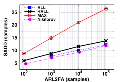
(a) $\mathsf{SADD}$ vs $\mathsf{ARL2FA}$ for the Boolean model

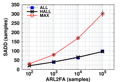
(b) $\mathsf{SADD}$ vs $\mathsf{ARL2FA}$ for the square law path loss model

Figure 5: $\mathsf{SADD}$ versus $\mathsf{ARL2FA}$ (for $\mathsf{PFI}\leqslant 5\times 10^{-2}$) for $\sf{MAX}$, $\sf{HALL}$, $\sf{ALL}$ and Nikiforov’s procedure for the Boolean and the square law path loss sensing models. In the Boolean sensing model, the system parameters are $f_{0}\sim{N}(0,1)$, $f_{1}\sim{N}(0,1)$, and in the case of path loss sensing model, the parameters are $f_{0}\sim{N}(0,1)$, $h_{e}=1$, $r_{d}=1.0$, $r_{i}=1.5$.

TABLE I: Simulation parameters and results for the Boolean sensing model for $\mathsf{PFI}\leqslant 5\times 10^{-2}$

Detection/	No. of	Threshold		99% Confidence interval			99% Confidence interval
Isolation	MC	$c$	$\mathsf{ARL2FA}$	$\mathsf{ARL2FA}_{\text{lower}}$	$\mathsf{ARL2FA}_{\text{upper}}$	$\mathsf{SADD}$	$\mathsf{SADD}_{\text{lower}}$	$\mathsf{SADD}_{\text{upper}}$
procedure	runs
MAX	$10^{4}$	2.71	$10^{2}$	93.69	106.61	8.77	8.45	9.09
	$10^{4}$	4.93	$10^{3}$	942.10	1065.81	14.89	14.41	15.37
	$10^{4}$	7.24	$10^{4}$	9398.61	10640.99	21.01	20.42	21.61
	$10^{4}$	9.52	$10^{5}$	95696.90	108008.89	26.43	25.76	27.11
HALL	$10^{4}$	1.67	$10^{2}$	92.67	107.58	5.96	5.72	6.20
	$10^{4}$	2.69	$10^{3}$	927.17	1085.48	8.81	8.48	9.14
	$10^{4}$	3.66	$10^{4}$	9239.97	10826.71	11.58	11.17	11.99
	$10^{4}$	4.52	$10^{5}$	92492.85	108389.15	13.78	13.32	14.23
ALL	$10^{4}$	2.16	$10^{3}$	915.94	1089.33	7.82	7.53	8.11
	$10^{4}$	2.96	$10^{4}$	9197.23	10811.90	10.07	9.70	10.44
	$10^{4}$	3.71	$10^{5}$	92205.45	107952.43	12.20	11.76	12.63
Nikiforov	$10^{4}$	2.75	$10^{2}$	98.30	116.32	4.75	4.52	4.98
	$10^{4}$	4.50	$10^{3}$	986.48	1048.23	7.08	6.79	7.38
	$10^{4}$	6.32	$10^{4}$	9727.19	10261.94	9.14	9.00	9.68
	$10^{4}$	8.32	$10^{5}$	98961.41	110415.50	11.28	11.00	12.25

TABLE II: Simulation parameters and results for the square law path loss sensing model for $\mathsf{PFI}\leqslant 5\times 10^{-2}$

Detection/	No. of	Threshold		99% Confidence interval			99% Confidence interval
Isolation	MC	$c$	$\mathsf{ARL2FA}$	$\mathsf{ARL2FA}_{\text{lower}}$	$\mathsf{ARL2FA}_{\text{upper}}$	$\mathsf{SADD}$	$\mathsf{SADD}_{\text{lower}}$	$\mathsf{SADD}_{\text{upper}}$
procedure	runs
MAX	$10^{4}$	2.71	$10^{2}$	93.69	106.61	30.74	29.31	32.17
	$10^{4}$	4.93	$10^{3}$	942.10	1065.81	79.60	75.86	83.34
	$10^{4}$	7.23	$10^{4}$	9398.61	10640.99	169.63	161.61	177.65
	$10^{4}$	9.52	$10^{5}$	95696.90	108008.89	301.77	286.88	316.66
HALL	$10^{4}$	1.67	$10^{2}$	92.67	107.58	20.58	19.43	21.74
	$10^{4}$	2.69	$10^{3}$	927.17	1085.48	40.56	38.24	42.88
	$10^{4}$	3.66	$10^{4}$	9239.97	10826.71	66.45	62.57	70.33
	$10^{4}$	4.52	$10^{5}$	92492.85	108389.15	96.93	91.03	102.82
ALL	$10^{4}$	1.33	$10^{2}$	92.24	107.79	20.19	19.06	21.32
	$10^{4}$	2.16	$10^{3}$	915.94	1089.33	39.90	37.59	42.21
	$10^{4}$	2.96	$10^{4}$	9197.23	10811.90	63.34	59.43	67.24
	$10^{4}$	3.71	$10^{5}$	92205.45	107952.43	98.96	93.01	104.92

For the same sensor deployment in Fig. 4, we compute the $\mathsf{SADD}$ and the $\mathsf{ARL2FA}$ for the square law path loss ($\eta=2$) sensing model given in Section II. Also, the signal strength $h_{e}$ is taken to be unity. Thus, the sensor sets (${\cal N}_{i}$s) and the detection subregions (${\cal A}_{i}$s) are the same as in the Boolean model, we described above. Since $r_{d}$ is taken as 1, $f_{1}(\cdot;r_{d})\sim{\cal N}(1,1)$. Thus, the LLR of observation $X_{k}^{(s)}$ is given by $\ln\left(\frac{f_{1}(X_{k}^{(s)};r_{d})}{f_{0}(X_{k}^{(s)})}\right)=X_{k}^{(s)}-\frac{1}{2}$, which is the same as that in the Boolean sensing model. Hence, under the event not occurred hypothesis, the $\mathsf{ARL2FA}$ under the path loss sensing model is the same as that of the Boolean sensing model. The $\mathsf{CUSUM}$ threshold $c$ that yields the target $\mathsf{ARL2FA}$s and other parameters and results are tabulated in Table II. To obtain the $\mathsf{SADD}$ the event is assumed to occur at time 1, and at a distance of $r_{i}$ from all the nodes of ${\cal N}_{i}$ that influence covers the event (which corresponds to the maximum detection delay). We plot the $\mathsf{SADD}$ vs $\log(\mathsf{ARL2FA})$ in Fig. 5(b). The ordering on $\mathsf{SADD}$ for any $\mathsf{ARL2FA}$ across the procedures is the same as that in the Boolean model, and can be explained in the same manner. The ambiguity in $\ell_{e}$ affects $f_{1}(\cdot;d_{e,s})$ and shows up as large $\mathsf{SADD}$ values.

VI Conclusion

We consider the quickest distributed event detection/isolation problem in a large extent $\mathsf{WSN}$ with a practical sensing model which incorporates the reduction in signal strength with distance. We formulate the change detection/isolation problem in the optimality framework of [2] and [3]. We propose distributed detection/isolation procedures, $\sf{MAX}$, $\sf{ALL}$ and $\sf{HALL}$ and show that as $\min\{\mathsf{ARL2FA},1/\mathsf{PFI}\}\to\infty$, the $\mathsf{SADD}$ performance of the distributed procedures grows in the same scale as that of the optimal centralised procedure of Tartakovsky [3] and Nikiforov [2].

Appendix A Proof of Theorem 2

From detection sensor sets ${\cal N}_{i},i=1,2,\cdots,N$, we choose the collection of indices ${\cal I}\subseteq\{1,2,\cdots,N\}$ such that any two sensor sets ${\cal N}_{i}$, ${\cal N}_{j}$, $i,j\in{\cal I}$, are not partially ordered by set inclusion. For each $i\in{\cal I}$, define the set of sensors that are unique to the sensor set ${\cal N}_{i}$, ${\cal M}_{i}\ :=\ {\cal N}_{i}\setminus\underset{j\neq i,j\in{\cal I}}{\bigcup}{\cal N}_{j}\ \subseteq{\cal N}_{i}$. The sets ${\cal M}_{1},{\cal M}_{2},\cdots,{\cal M}_{|{\cal I}|}$ are disjoint. Under the null hypothesis, ${\bf H}_{0}$, the observations of sensors in the sensor sets ${\cal M}_{1},{\cal M}_{2},\cdots,{\cal M}_{|{\cal I}|}$ are iid, with the pdf $f_{0}\sim{\cal N}(0,\sigma^{2})$. For every ${\cal N}_{i}$, there exists ${\cal M}_{j}$ such that ${\cal M}_{j}\subseteq{\cal N}_{i}$, so that $\tau^{{\sf rule},({\cal N}_{i})}\geqslant\tau^{{\sf rule},({\cal M}_{j})}$. Hence, $\tau^{\sf procedure}=\min\{\tau^{{\sf procedure},({\cal N}_{i})}:i=1,2,\cdots,N\}\geqslant\min\{\tau^{{\sf procedure},({\cal M}_{i})}:i\in{\cal I}\}=:\widehat{\tau}^{\ {\sf rule}}$. Hence,

$$\mathsf{E}_{\infty}\left[\tau^{{\sf rule}}\right] \geqslant\mathsf{E}_{\infty}\left[\widehat{\tau}^{\ {\sf rule}}\right]\ \geqslant e^{mc}\cdot\mathsf{P}\left\{\widehat{\tau}^{\ {\sf rule}}>e^{mc}\right\}\ \text{(by the Markov inequality)}$$

$$\text{or,}\ \frac{\mathsf{E}_{\infty}\left[\tau^{{\sf rule}}\right]}{e^{mc}} \geqslant\mathsf{P}\left\{\widehat{\tau}^{\ {\sf rule}}>e^{mc}\right\}\ =\ \prod_{i\in{\cal I}}\mathsf{P}_{\infty}\left\{\tau^{\ {\sf rule},({\cal M}_{i})}>e^{mc}\right\}.$$ (27)

We analyse $\mathsf{P}_{\infty}\left\{\tau^{\ {\sf rule},({\cal M}_{i})}>e^{mc}\right\}$ as $c\to\infty$, for $\mathsf{ALL}$, $\mathsf{MAX}$, and $\mathsf{HALL}$. For ${\sf ALL}$,

$$\mathsf{P}_{\infty}\left\{\tau^{\ {\sf ALL},({\cal M}_{i})}=k\right\} \leqslant\ \mathsf{P}_{\infty}\left\{C_{k}^{(s)}\geqslant c,\forall s\in{\cal M}_{i}\right\}\ \ =\ \prod_{s\in{\cal M}_{i}}\mathsf{P}_{\infty}\left\{C_{k}^{(s)}\geqslant c\right\}$$

$${\leqslant}\ e^{-cm_{i}}\ \ \ \ \text{(using Wald's inequality)}$$

$$\text{Therefore},\hskip 28.45274pt\mathsf{P}_{\infty}\left\{\tau^{\ {\sf ALL},({\cal M}_{i})}\leqslant k\right\} \leqslant k\cdot e^{-cm_{i}}$$

$$\mathsf{P}_{\infty}\left\{\tau^{\ {\sf ALL},({\cal M}_{i})}>e^{mc}\right\} \geqslant 1-e^{-c(m_{i}-m)}.$$

Hence, for any $m<m_{i}$, we have $\liminf_{c\to\infty}\ \mathsf{P}_{\infty}\left\{\tau^{\ {\sf ALL},({\cal M}_{i})}>e^{mc}\right\}=1$. A large $m$ (which is smaller than all $m_{i}$s) is desirable. Thus, a good choice for $m$ is $a_{\sf ALL}=\min\{m_{i}:i\in{\cal I}\}-\delta$. for some arbitrarily small $\delta>0$. Hence, from Eqn. (27),

$$\mathsf{E}_{\infty}\left[\tau^{\sf ALL}\right] \geqslant\exp\left(a_{\sf ALL}c\right)(1+o(1))$$ (28)

For ${\sf MAX}$, at the stopping time of $\mathsf{MAX}$, at least one of the ${\sf CUSUM}$ statistics is above the threshold $c$,

$$\mathsf{P}_{\infty}\left\{\tau^{\ {\sf MAX},({\cal M}_{i})}=k\right\} \leqslant\mathsf{P}_{\infty}\left\{C_{k}^{(s)}\geqslant c,\ \text{for some}\ s\in{\cal M}_{i}\right\}$$

$$\leqslant\sum_{s\in{\cal M}_{i}}\mathsf{P}_{\infty}\left\{C_{k}^{(s)}\geqslant c\right\}$$

$${\leqslant}m_{i}e^{-c}\ \ \ \ \text{(using Wald's inequality)}.$$ (29)

$$\text{Therefore, for any arbitrarily small $\delta>0$},\ \mathsf{P}_{\infty}\left\{\tau^{\ {\sf MAX},({\cal M}_{i})}>e^{(1-\delta)c}\right\} \geqslant 1-m_{i}e^{-\delta c}$$

$$\liminf_{c\to\infty}\mathsf{P}_{\infty}\left\{\tau^{\ {\sf MAX},({\cal M}_{i})}>e^{(1-\delta)c}\right\} =1.$$ (30)

Let $a_{\sf MAX}=1-\delta$. For any arbitrarily small $\delta>0$, we see from Eqn. (27),

$$\mathsf{E}_{\infty}\left[\tau^{{\sf MAX}}\right]\geqslant\exp\left((1-\delta)c\right)(1+o(1))\ \ =:\ \exp\left(a_{\sf MAX}c\right)(1+o(1)),$$ (31)

For HALL, for the same threshold $c$, the stopping time of $\mathsf{HALL}$ is after that of $\mathsf{MAX}$. Hence, $\tau^{\ {\sf HALL}}\ \geqslant\ \tau^{\ {\sf MAX}}$. Hence, $\mathsf{E}_{\infty}\left[\tau^{\ {\sf HALL}}\right]\ \geqslant\ \mathsf{E}_{\infty}\left[\tau^{\ {\sf MAX}}\right]\ \geqslant\ \exp\left((1-\delta)c\right)(1+o(1))$ (from Eqn. (31)). Thus, for $a_{\sf ALL}:=1-\delta$, for any arbitrarily small $\delta>0$,

$$\mathsf{E}_{\infty}\left[\tau^{\ {\sf HALL}}\right] \geqslant\exp\left(a_{\sf ALL}c\right)(1+o(1))$$ (32)

Appendix B Proof of Theorem 3

Consider $\ell_{e}\in{\cal A}_{i}$. The probability of false isolation when the detection is due to ${\cal N}_{j}\not\subseteq{\cal N}(\ell_{e})$ is

$${\sf P}_{1}^{({\bf d}(\ell_{e}))}\left\{\tau^{{\sf rule}}=\tau^{{\sf rule},({\cal N}_{j})}\right\} ={\sf P}_{1}^{({\bf d}(\ell_{e}))}\left\{\tau^{{\sf rule},({\cal N}_{j})}\leqslant\tau^{{\sf rule},({\cal N}_{h})},\forall h=1,2,\cdots,N\right\}$$

$$\leqslant{\sf P}_{1}^{({\bf d}(\ell_{e}))}\left\{\tau^{{\sf rule},({\cal N}_{j})}\leqslant\tau^{{\sf rule},({\cal N}_{i})}\right\}$$

$$=\sum_{k=1}^{\infty}{\sf P}_{1}^{({\bf d}(\ell_{e}))}\left\{\tau^{{\sf rule},({\cal N}_{i})}=k\right\}{\sf P}_{1}^{({\bf d}(\ell_{e}))}\left\{\tau^{{\sf rule},({\cal N}_{j})}\leqslant k\mid\tau^{{\sf rule},({\cal N}_{i})}=k\right\}$$

$$=\sum_{k=1}^{\infty}{\sf P}_{1}^{({\bf d}(\ell_{e}))}\left\{\tau^{{\sf rule},({\cal N}_{i})}=k\right\}\left[\sum_{t=1}^{k}{\sf P}_{1}^{({\bf d}(\ell_{e}))}\left\{\tau^{{\sf rule},({\cal N}_{j})}=t\mid\tau^{{\sf rule},({\cal N}_{i})}=k\right\}\right]$$

B-A ${\sf PFI}(\tau^{\sf ALL})$ – Boolean Sensing Model

$${\sf P}_{1}^{(i)}\left\{\tau^{\mathsf{ALL},({\cal N}_{j})}=t\mid\tau^{\mathsf{ALL},({\cal N}_{i})}=k\right\} \leqslant{\sf P}_{1}^{(i)}\left\{C_{t}^{(s)}\geqslant c,\ \forall s\in{\cal N}_{j}\mid\tau^{\mathsf{ALL},({\cal N}_{i})}=k\right\}$$

$$\leqslant{\mathsf{P}}_{\infty}\left\{C_{t}^{(s)}\geqslant c,\ \forall s\in{\cal N}_{j}\setminus{\cal N}_{i}\right\}$$

$$\leqslant\exp\left(-|{\cal N}_{j}\setminus{\cal N}_{i}|c\right)\ \ \ \text{(using Wald's inequality)}.$$

$$\text{Therefore,}\ {\sf P}_{1}^{(i)}\left\{\tau^{{\mathsf{ALL}},({\cal N}_{j})}\leqslant\tau^{\mathsf{ALL},({\cal N}_{i})}\right\} \leqslant\exp\left(-|{\cal N}_{j}\setminus{\cal N}_{i}|c\right)\cdot{\mathsf{E}}_{1}^{(i)}\left[\tau^{\mathsf{ALL},({\cal N}_{i})}\right]$$

$$\leqslant\exp\left(-(|{\cal N}_{j}\setminus{\cal N}_{i}|c-\ln(c))\right)\cdot\frac{1}{\alpha|{\cal N}_{i}|}(1+o(1)).$$

$$\text{Hence},\ {\sf PFI}(\tau^{\mathsf{ALL}}) \leqslant\ \max_{1\leqslant i\leqslant N}\ \max_{1\leqslant j\leqslant N,{\cal N}_{j}\not\subseteq{\cal N}_{i}}\ {\mathsf{P}}_{1}^{(i)}\left\{\tau^{{\mathsf{ALL}},({\cal N}_{j})}\leqslant\tau^{\mathsf{ALL},({\cal N}_{i})}\right\}$$

$$\leqslant\frac{\exp\left(-(mc-\ln(c))\right)}{\underline{n}\alpha}(1+o(1))$$ (33)

where $\underline{n}=\min\{|{\cal N}_{i}:i=1,2,\cdots,N|\}$, $m=\underset{1\leqslant i\leqslant N,1\leqslant j\leqslant N,{\cal N}_{j}\not\subseteq{\cal N}_{i}}{\min}\{|{\cal N}_{j}\setminus{\cal N}_{i}|\}$. For any $n$, there exists $c_{0}(n)$ such that for all $c>c_{0}(n),c<e^{c/n}$. Using this inequality, for sufficiently large $c$

$${\sf PFI}(\tau^{\mathsf{ALL}}) \leqslant\frac{\exp\left(-\left(\left(m-\frac{1}{n}\right)c\right)\right)}{\underline{n}\alpha}(1+o(1))\ =\frac{\exp(-b_{\mathsf{ALL}}\cdot c)}{B_{\sf\mathsf{ALL}}}(1+o(1)),$$

where $b_{\sf\mathsf{ALL}}=m-1/n$ and $B_{\mathsf{ALL}}=\underline{n}\alpha$.

B-B ${\sf PFI}(\tau^{\sf MAX})$ – Boolean Sensing Model

$${\mathsf{P}}_{1}^{(i)}\left\{\tau^{{\sf MAX},({\cal N}_{j})}=t\mid\tau^{\mathsf{MAX},({\cal N}_{i})}=k\right\} \leqslant{\mathsf{P}}_{1}^{(i)}\left\{\tau^{(s)}\leqslant t,\forall s\in{\cal N}_{j}\mid\tau^{\mathsf{MAX},({\cal N}_{i})}=k\right\}$$

$$\leqslant{\mathsf{P}}_{\infty}\left\{\tau^{(s)}\leqslant t,\forall s\in{\cal N}_{j}\setminus{\cal N}_{i}\mid\tau^{\mathsf{MAX},({\cal N}_{i})}=k\right\}$$

$$=\prod_{s\in{\cal N}_{j}\setminus{\cal N}_{i}}\ \sum_{n=1}^{t}\ {\mathsf{P}}_{\infty}\left\{\tau^{(s)}=n\mid\tau^{\mathsf{MAX},({\cal N}_{i})}=k\right\}$$

$$=\prod_{s\in{\cal N}_{j}\setminus{\cal N}_{i}}\ \sum_{n=1}^{t}\ {\mathsf{P}}_{\infty}\left\{C_{n}^{(s)}\geqslant c\right\}$$

$$\leqslant\exp\left(-m_{ji}c\right)t^{m_{ji}}$$

$$\text{Hence,}\ {\mathsf{P}}_{1}^{(i)}\left\{\tau^{\sf MAX,({\cal N}_{j})}\leqslant\tau^{\mathsf{MAX},({\cal N}_{i})}\right\} \leqslant\exp\left(-m_{ji}c\right){\mathsf{E}}_{1}^{(i)}\left[(\tau^{\mathsf{MAX},{\cal N}_{i}})^{1+m_{ji}}\right]$$

$$\leqslant\exp\left(-m_{ji}c\right)\frac{c^{1+m_{ji}}}{\alpha^{1+m_{ji}}}(1+o(1))$$

$$=\frac{\exp\left(-\left(m_{ji}c-(1+m_{ji})\ln(c)\right)\right)}{\alpha^{1+m_{ji}}}(1+o(1))$$

Let $m=\underset{1\leqslant i\leqslant N,1\leqslant j\leqslant N,{\cal N}_{j}\not\subseteq{\cal N}_{i}}{\min}m_{ji}$, $\bar{m}=\underset{1\leqslant i\leqslant N,1\leqslant j\leqslant N,{\cal N}_{j}\not\subseteq{\cal N}_{i}}{\max}m_{ji}$, and $\alpha^{*}=\underset{1\leqslant i\leqslant N,1\leqslant j\leqslant N,{\cal N}_{j}\not\subseteq{\cal N}_{i}}{\min}\alpha^{1+m_{ji}}$.

$$\text{Therefore,}\ {\sf PFI}(\tau^{\mathsf{MAX}}) \leqslant\max_{1\leqslant i\leqslant N}\ \max_{1\leqslant j\leqslant N,{\cal N}_{j}\not\subseteq{\cal N}_{i}}\ {\mathsf{P}}_{1}^{(i)}\left\{\tau^{\sf MAX,({\cal N}_{j})}\leqslant\tau^{\mathsf{MAX},({\cal N}_{i})}\right\}$$

$$\leqslant\frac{\exp\left(-\left(mc-(1+\bar{m})\ln(c)\right)\right)}{\alpha^{*}}(1+o(1)).$$

For any $n$, there exists $c_{0}(n)$ such that for all $c>c_{0}(n),c<e^{c/n}$. Hence, for sufficiently large $c$

$${\sf PFI}(\tau^{\mathsf{MAX}}) \leqslant\max_{1\leqslant i\leqslant N}\ \max_{1\leqslant j\leqslant N,{\cal N}_{j}\not\subseteq{\cal N}_{i}}\ {\mathsf{P}}_{T}^{(i)}\left\{\tau^{\sf MAX,({\cal N}_{j})}\leqslant\tau^{\mathsf{MAX},({\cal N}_{i})}\right\}$$

$$\leqslant\frac{\exp\left(-\left(m-\frac{1+\bar{m}}{n}\right)c\right)}{\alpha^{*}}(1+o(1))\ =\ \frac{\exp(-b_{\mathsf{MAX}}\cdot c)}{B_{\sf\mathsf{MAX}}}(1+o(1)),$$

where $b_{\sf\mathsf{MAX}}=m-((1+\bar{m})/n)$ and $B_{\mathsf{MAX}}=\alpha^{*}$.

B-C ${\sf PFI}(\tau^{\sf HALL})$ – Boolean Sensing Model

$${\mathsf{P}}_{1}^{(i)}\left\{\tau^{{\sf HALL},({\cal N}_{j})}=t\mid\tau^{\mathsf{HALL},({\cal N}_{i})}=k\right\} \leqslant{\mathsf{P}}_{1}^{(i)}\left\{\tau^{(s)}\leqslant t,\forall s\in{\cal N}_{j}\mid\tau^{\mathsf{HALL},({\cal N}_{i})}=k\right\}$$

which has the same form as that of $\mathsf{MAX}$. Hence, from the analysis of $\mathsf{MAX}$, it follows that

$${\mathsf{P}}_{1}^{(i)}\left\{\tau^{\sf HALL,({\cal N}_{j})}\leqslant\tau^{\mathsf{HALL},({\cal N}_{i})}\right\} \leqslant\exp\left(-m_{ji}c\right){\mathsf{E}}_{1}^{(i)}\left[(\tau^{\mathsf{HALL},({\cal N}_{i})})^{1+m_{ji}}\right]$$

$$\leqslant\exp\left(-m_{ji}c\right)\frac{c^{1+m_{ji}}}{|{\cal N}_{i}|^{1+m_{ji}}\alpha^{1+m_{ji}}}(1+o(1))$$

$$=\exp\left(-\left(m_{ji}c-(1+m_{ji})\ln(c)\right)\right)\left[\frac{1}{\alpha|{\cal N}_{i}|}\right]^{1+m_{ji}}(1+o(1))$$

$${\sf PFI}(\tau^{\mathsf{HALL}}) \leqslant\ \max_{1\leqslant i\leqslant N}\ \max_{1\leqslant j\leqslant N,{\cal N}_{j}\not\subseteq{\cal N}_{i}}\ {\mathsf{P}}_{1}^{(i)}\left\{\tau^{\sf HALL,({\cal N}_{j})}\leqslant\tau^{\mathsf{HALL},({\cal N}_{i})}\right\}$$

$$\leqslant\frac{\exp\left(-\left(mc-(1+\bar{m})\ln(c)\right)\right)}{\alpha^{*}}(1+o(1)).$$

where $\alpha^{*}=\underset{1\leqslant i\leqslant N,1\leqslant j\leqslant N,{\cal N}_{j}\not\subseteq{\cal N}_{i}}{\min}\left(\alpha\cdot|{\cal N}_{i}|\right)^{1+m_{ji}}$. For any $n$ there exists $c_{0}(n)$ such that for all $c>c_{0}(n),c<e^{c/n}$. Hence, for sufficiently large $c$

$${\sf PFI}(\tau^{\mathsf{HALL}}) \leqslant\ \max_{1\leqslant i\leqslant N}\ \max_{1\leqslant j\leqslant N,{\cal N}_{j}\not\subseteq{\cal N}_{i}}\ {\mathsf{P}}_{1}^{(i)}\left\{\tau^{\sf HALL,({\cal N}_{j})}\leqslant\tau^{\mathsf{HALL},({\cal N}_{i})}\right\}$$

$$\leqslant\frac{\exp\left(-\left(m-\frac{1+\bar{m}}{n}\right)c\right)}{\alpha^{*}}(1+o(1))\ =\ \frac{\exp(-b_{\mathsf{HALL}}\cdot c)}{B_{\sf\mathsf{HALL}}}(1+o(1)),$$

where $b_{\sf\mathsf{HALL}}=m-((1+\bar{m})/n)$ and $B_{\mathsf{HALL}}=\alpha^{*}$.

$\mathsf{PFI}$ – Path–Loss Sensing Model

Lemma 2

For $s\in{\cal N}_{j}\setminus{\cal M}_{e}$ and for $t\geqslant T$, (with the pre–change pdf $f_{0}\sim{\cal N}(0,\sigma^{2})$ and the post–change pdf $f_{1}\sim{\cal N}(h_{e}\rho(r_{s}),\sigma^{2})$)

$${\sf P}_{1}^{({\bf d}(\ell_{e}))}\left\{C_{t}^{(s)}\geqslant c\right\} \leqslant\exp\left(-\frac{\underline{\omega}_{0}}{2}c\right)\cdot\frac{\exp\left(-\frac{\alpha\underline{\omega}_{0}^{2}}{4}\right)}{1-\exp\left(-\frac{\alpha\underline{\omega}_{0}^{2}}{4}\right)},$$

where we recall that the parameter $\underline{\omega}_{0}$ defines the influence range, and $\alpha=$ KL$(f_{1},f_{0})$.

Proof: For $s\in{\cal N}_{j}\setminus{\cal M}_{e}$ and for $t\geqslant T$,

$${\sf P}_{1}^{({\bf d}(\ell_{e}))}\left\{C_{t}^{(s)}\geqslant c\right\}$$

$$={\sf P}_{1}^{({\bf d}(\ell_{e}))}\left\{\max_{1\leqslant n\leqslant t}\sum_{k=1}^{n}\ln\left(\frac{f_{1}(X^{(s)}_{k};r_{s})}{f_{0}(X^{(s)}_{k})}\right)\geqslant c\right\}$$

$$\leqslant\sum_{n=1}^{\infty}{\sf P}_{1}^{({\bf d}(\ell_{e}))}\left\{\sum_{k=1}^{n}\ln\left(\frac{f_{1}(X^{(s)}_{k};r_{s})}{f_{0}(X^{(s)}_{k})}\right)\geqslant c\right\}$$

$$=\sum_{n=1}^{T-1}{\mathsf{P}}_{\infty}\left\{\sum_{k=1}^{n}\ln\left(\frac{f_{1}(X^{(s)}_{k};r_{s})}{f_{0}(X^{(s)}_{k})}\right)\geqslant c\right\}+\sum_{n=T}^{\infty}{\sf P}_{1}^{({\bf d}(\ell_{e}))}\left\{\sum_{k=1}^{n}\ln\left(\frac{f_{1}(X^{(s)}_{k};r_{s})}{f_{0}(X^{(s)}_{k})}\right)\geqslant c\right\}$$

$$=\sum_{n=1}^{T-1}{\mathsf{P}}_{\infty}\left\{\sum_{k=1}^{n}\ln\left(\frac{f_{1}(X^{(s)}_{k};r_{s})}{f_{0}(X^{(s)}_{k})}\right)\geqslant c\right\}+\sum_{n=T}^{\infty}{\sf P}_{1}^{({\bf d}(\ell_{e}))}\left\{\sum_{k=1}^{T-1}\ln\left(\frac{f_{1}(X^{(s)}_{k};r_{s})}{f_{0}(X^{(s)}_{k})}\right)+\sum_{k=T}^{n}\ln\left(\frac{f_{1}(X^{(s)}_{k};r_{s})}{f_{0}(X^{(s)}_{k})}\right)\geqslant c\right\}$$

$$=\sum_{n=1}^{T-1}{\mathsf{P}}_{\infty}\left\{\sum_{k=1}^{n}X_{k}^{(s)}\geqslant\frac{\sigma^{2}}{h_{e}\rho(r_{s})}(c+n\alpha)\right\}+\sum_{n=T}^{\infty}{\mathsf{P}}_{\infty}\left\{\sum_{k=1}^{n}X_{k}^{(s)}\geqslant\frac{\sigma^{2}}{h_{e}\rho(r_{s})}c+nh_{e}\left(\frac{\rho(r_{s})}{2}-\rho(d_{e,s})\right)+\left(T-1\right)h_{e}\rho(d_{e,s})\right\}$$

$$\leqslant\sum_{n=1}^{T-1}{\mathsf{P}}_{\infty}\left\{\sum_{k=1}^{n}X_{k}^{(s)}\geqslant\frac{\sigma^{2}}{h_{e}\rho(r_{s})}(c+n\alpha)\right\}+\sum_{n=T}^{\infty}{\mathsf{P}}_{\infty}\left\{\sum_{k=1}^{n}X_{k}^{(s)}\geqslant n\cdot{h_{e}\frac{\rho(r_{s})}{2}\underline{\omega}_{0}}+{c\cdot\frac{\sigma^{2}}{h_{e}\rho(r_{s})}}\right\}$$

$$\leqslant\sum_{n=1}^{\infty}{\mathsf{P}}_{\infty}\left\{\exp\left(\theta\sum_{k=1}^{n}X_{k}^{(s)}\right)\geqslant\exp\left(\frac{\theta\sigma^{2}}{h_{e}\rho(r_{s})}(c+n\alpha\underline{\omega}_{0})\right)\right\}\ \ \text{for any}\ \theta>0.$$

$$\text{Hence},\ {\sf P}_{1}^{({\bf d}(\ell_{e}))}\left\{C_{t}^{(s)}\geqslant c\right\} \leqslant\sum_{n=1}^{\infty}\exp\left(-\frac{\theta\sigma^{2}}{h_{e}\rho(r_{s})}(c+n\alpha\underline{\omega}_{0})\right)\left({\mathsf{E}}_{\infty}\left[e^{\theta X_{1}^{(s)}}\right]\right)^{n}$$

$$=\sum_{n=1}^{\infty}\exp\left(-\frac{\theta\sigma^{2}}{h_{e}\rho(r_{s})}(c+n\alpha\underline{\omega}_{0})+\frac{n\sigma^{2}\theta^{2}}{2}\right)$$

Since the above inequality holds for any $\theta>0$, we have

$${\sf P}_{1}^{({\bf d}(\ell_{e}))}\left\{C_{t}^{(s)}\geqslant c\right\} \leqslant\sum_{n=1}^{\infty}\min_{\theta>0}\exp\left(-\frac{\theta\sigma^{2}}{h_{e}\rho(r_{s})}(c+n\alpha\underline{\omega}_{0})+\frac{n\sigma^{2}\theta^{2}}{2}\right)$$

The minimising $\theta$ is $\frac{c+n\alpha\underline{\omega}_{0}}{nh_{e}\rho(r_{s})}$. Therefore, for $\theta=\frac{c+n\alpha\underline{\omega}_{0}}{nh_{e}\rho(r_{s})}$,

$${\sf P}_{1}^{({\bf d}(\ell_{e}))}\left\{C_{t}^{(s)}\geqslant c\right\} \leqslant\sum_{n=1}^{\infty}\exp\left(\frac{-(c+n\alpha\underline{\omega}_{0})^{2}}{4\alpha n}\right).$$

$$\text{Note that}\ -\frac{(c+\alpha\underline{\omega}_{0}n)^{2}}{4\alpha n}+\frac{(c+\alpha\underline{\omega}_{0}(n-1))^{2}}{4\alpha(n-1)} =-\frac{\alpha\underline{\omega}_{0}^{2}}{4}+\frac{c^{2}}{4\alpha(n-1)n}$$

Therefore, by iteratively computing the exponent, we have

$$\exp\left(-\frac{(c+\alpha\underline{\omega}_{0}n)^{2}}{4\alpha n}\right) =\exp\left(-\frac{(c+\alpha\underline{\omega}_{0})^{2}}{4\alpha}\right)\cdot\exp\left(-\frac{\alpha\underline{\omega}_{0}^{2}}{4}(n-1)\right)\exp\left(\frac{c^{2}}{4\alpha}\left(1-\frac{1}{n}\right)\right)$$

$$\leqslant\exp\left(-\frac{(c+\alpha\underline{\omega}_{0})^{2}}{4\alpha}\right)\cdot\exp\left(-\frac{\alpha\underline{\omega}_{0}^{2}}{4}(n-1)\right)\exp\left(\frac{c^{2}}{4\alpha}\right)$$

$$\text{or}\ \sum_{n=1}^{\infty}\exp\left(-\frac{(c+\alpha\underline{\omega}_{0}n)^{2}}{4\alpha n}\right) \leqslant\exp\left(-\frac{\underline{\omega}_{0}}{2}c\right)\cdot\frac{\exp\left(-\frac{\alpha\underline{\omega}_{0}^{2}}{4}\right)}{1-\exp\left(-\frac{\alpha\underline{\omega}_{0}^{2}}{4}\right)}$$

$$=:\beta$$

B-D ${\sf PFI}(\tau^{\sf ALL})$ – Path Loss Sensing Model

$${\sf P}_{1}^{({\bf d}(\ell_{e}))}\left\{\tau^{\sf ALL,({\cal N}_{j})}=t\mid\tau^{\mathsf{ALL},({\cal N}_{i})}=k\right\} \leqslant{\sf P}_{1}^{({\bf d}(\ell_{e}))}\left\{C_{t}^{(s)}\geqslant c,\forall s\in{\cal N}_{j}\mid\tau^{\mathsf{ALL},({\cal N}_{i})}=k\right\}$$

$$\leqslant{\sf P}_{1}^{({\bf d}(\ell_{e}))}\left\{C_{t}^{(s)}\geqslant c,\forall s\in{\cal N}_{j}\setminus{\cal N}(\ell_{e})\mid\tau^{\mathsf{ALL},({\cal N}_{i})}=k\right\}$$

$$=\prod_{s\in{\cal N}_{j}\setminus{\cal N}(\ell_{e})}{\sf P}_{1}^{({\bf d}(\ell_{e}))}\left\{C_{t}^{(s)}\geqslant c\right\}$$

$$\leqslant\beta^{|{\cal N}_{j}\setminus{\cal N}(\ell_{e})|}\ \ \ (\text{from Lemma~{}\ref{lem:path-bound}})$$

$$\text{Therefore},\ {\sf P}_{1}^{({\bf d}(\ell_{e}))}\left\{\tau^{\sf ALL,({\cal N}_{j})}\leqslant\tau^{\mathsf{ALL},({\cal N}_{i})}\right\} \leqslant\beta^{{|{\cal N}_{j}\setminus{\cal N}(\ell_{e})|}}{\mathsf{E}}_{1}^{({\bf d}(\ell_{e}))}\left[\tau^{\mathsf{ALL},({\cal N}_{i})}\right]$$

$$\leqslant\beta^{{|{\cal N}_{j}\setminus{\cal N}(\ell_{e})|}}\frac{c}{\alpha|{\cal N}_{i}|}(1+o(1))$$

Let $m=\underset{1\leqslant i\leqslant N,\ell_{e}\in{\cal A}_{i},1\leqslant j\leqslant N,{\cal N}_{j}\not\subseteq{\cal N}(\ell_{e})}{\min}|{\cal N}_{j}\setminus{\cal N}(\ell_{e})|$ and $\underline{n}=\min\{|{\cal N}_{i}|:i=1,2,\cdots,N\}$. Define $K=\underset{1\leqslant i\leqslant N,\ell_{e}\in{\cal A}_{i},1\leqslant j\leqslant N,{\cal N}_{j}\not\subseteq{\cal N}(\ell_{e})}{\max}\left[\frac{\exp\left(-\frac{\alpha\underline{\omega}_{0}^{2}}{4}\right)}{1-\exp\left(-\frac{\alpha\underline{\omega}_{0}^{2}}{4}\right)}\right]^{|{\cal N}_{j}\setminus{\cal N}(\ell_{e})|}$. Therefore,

$${\mathsf{PFI}}\left(\tau^{\sf ALL}\right) \leqslant\ \max_{1\leqslant i\leqslant N}\ \sup_{\ell_{e}\in{\cal A}_{i}}\ \max_{1\leqslant j\leqslant N,{\cal N}_{j}\not\subseteq{\cal N}(\ell_{i})}\ {\sf P}_{1}^{({\bf d}(\ell_{e}))}\left\{\tau^{\sf ALL,({\cal N}_{j})}\leqslant\tau^{\mathsf{ALL},({\cal N}_{i})}\right\}$$

$$\leqslant\frac{K\exp\left(-\left(\frac{m\underline{\omega}_{0}}{2}c-\ln(c)\right)\right)}{\alpha\underline{n}}(1+o(1)).$$

For any $n$ there exists $c_{0}(n)$ such that for all $c>c_{0}(n),c<e^{c/n}$. Hence, for sufficiently large $c$

$${\mathsf{PFI}}\left(\tau^{\sf ALL}\right) \leqslant\frac{K\exp\left(-\left(\frac{m\underline{\omega}_{0}}{2}-\frac{1}{n}\right)c\right)}{\alpha\underline{n}}(1+o(1))\ =\ \frac{\exp(-b_{\mathsf{ALL},d}\cdot c)}{B_{\sf\mathsf{ALL},d}}(1+o(1))$$

where $b_{\mathsf{ALL},d}=(m\underline{\omega}_{0}/2)-(1/n)$ and $B_{\mathsf{ALL},d}=\alpha\underline{n}/K$.

B-E ${\sf PFI}(\tau^{\sf MAX})$ – Path Loss Sensing Model

$${\sf P}_{1}^{({\bf d}(\ell_{e}))}\left\{\tau^{\sf MAX,({\cal N}_{j})}=t\mid\tau^{\mathsf{MAX},({\cal N}_{i})}=k\right\} \leqslant{\sf P}_{1}^{({\bf d}(\ell_{e}))}\left\{\tau^{(s)}\leqslant t,\forall\ s\in{\cal N}_{j}\setminus{\cal N}(\ell_{e})\mid\tau^{\mathsf{MAX},({\cal N}_{i})}=k\right\}$$

$$=\prod_{s\in{\cal N}_{j}\setminus{\cal N}(\ell_{e})}\ {\sf P}_{1}^{({\bf d}(\ell_{e}))}\left\{\tau^{(s)}\leqslant t\mid\tau^{\mathsf{MAX},({\cal N}_{i})}=k\right\}$$

$$\leqslant\prod_{s\in{\cal N}_{j}\setminus{\cal N}(\ell_{e})}\ \sum_{n=1}^{t}\ {\sf P}_{1}^{({\bf d}(\ell_{e}))}\left\{C_{n}^{(s)}\geqslant c\right\}$$

$$\leqslant{\beta}^{|{\cal N}_{j}\setminus{\cal N}(\ell_{e})|}\cdot t^{|{\cal N}_{j}\setminus{\cal N}(\ell_{e})|}\ \ \ (\text{from Lemma~{}\ref{lem:path-bound}})$$

$${\sf P}_{1}^{({\bf d}(\ell_{e}))}\left\{\tau^{\sf MAX,({\cal N}_{j})}\leqslant\tau^{\mathsf{MAX},({\cal N}_{i})}\right\} \leqslant{\beta}^{|{\cal N}_{j}\setminus{\cal N}(\ell_{e})|}\cdot{\mathsf{E}}_{1}^{({\bf d}(\ell_{e}))}\left[(\tau^{\mathsf{MAX},({\cal N}_{i})})^{1+|{\cal N}_{j}\setminus{\cal N}(\ell_{e})|}\right]$$

$$\leqslant{\beta}^{|{\cal N}_{j}\setminus{\cal N}(\ell_{e})|}\cdot\frac{c^{1+|{\cal N}_{j}\setminus{\cal N}(\ell_{e})|}}{\alpha^{1+|{\cal N}_{j}\setminus{\cal N}(\ell_{e})|}}(1+o(1))$$

Let $m=\underset{1\leqslant i\leqslant N,\ell_{e}\in{\cal A}_{i},1\leqslant j\leqslant N,{\cal N}_{j}\not\subseteq{\cal N}(\ell_{e})}{\min}|{\cal N}_{j}\setminus{\cal N}(\ell_{e})|$, $\bar{m}=\underset{1\leqslant i\leqslant N,\ell_{e}\in{\cal A}_{i},1\leqslant j\leqslant N,{\cal N}_{j}\not\subseteq{\cal M}_{e}}{\max}|{\cal N}_{j}\setminus{\cal N}(\ell_{e})|$, and define $K=\underset{1\leqslant i\leqslant N,\ell_{e}\in{\cal A}_{i},1\leqslant j\leqslant N,{\cal N}_{j}\not\subseteq{\cal N}(\ell_{e})}{\max}\left[\frac{\exp\left(-\frac{\alpha\underline{\omega}_{0}^{2}}{4}\right)}{1-\exp\left(-\frac{\alpha\underline{\omega}_{0}^{2}}{4}\right)}\right]^{|{\cal N}_{j}\setminus{\cal N}(\ell_{e})|}$. Therefore,

$${\sf PFI}(\tau^{\mathsf{MAX}}) \leqslant\ \max_{1\leqslant i\leqslant N}\ \sup_{\ell_{e}\in{\cal A}_{i}}\ \max_{1\leqslant j\leqslant N,{\cal N}_{j}\not\subseteq{\cal N}(\ell_{e})}\ {\sf P}_{1}^{({\bf d}(\ell_{e}))}\left\{\tau^{\sf MAX,({\cal N}_{j})}\leqslant\tau^{\mathsf{MAX},({\cal N}_{i})}\right\}$$

$$\leqslant\frac{K}{\alpha^{*}}\exp\left(-\left(\frac{m\underline{\omega}_{0}}{2}c-(1+\bar{m})\ln(c)\right)\right)(1+o(1)).$$

where $\alpha^{*}=\underset{1\leqslant i\leqslant N,\ell_{e}\in{\cal A}_{i},1\leqslant j\leqslant N,{\cal N}_{j}\not\subseteq{\cal N}(\ell_{e})}{\min}\alpha^{1+|{\cal N}_{j}\setminus{\cal N}(\ell_{e})|}$. For any $n$ there exists $c_{0}(n)$ such that for all $c>c_{0}(n),c<e^{c/n}$. Hence, for sufficiently large $c$

$${\sf PFI}(\tau^{\mathsf{MAX}}) \leqslant\frac{K}{\alpha^{*}}\exp\left(-\left(\frac{m\underline{\omega}_{0}}{2}-\frac{1+\bar{m}}{n}\right)c\right)(1+o(1))\ =\ \frac{\exp(-b_{\mathsf{MAX},d}\cdot c)}{B_{\sf\mathsf{MAX},d}}(1+o(1)),$$

where $b_{\sf\mathsf{MAX},d}=(\frac{m\underline{\omega}_{0}}{2})-(\frac{1+\bar{m}}{n})$ and $B_{\mathsf{MAX},d}=\frac{\alpha^{*}}{K}$.

B-F ${\sf PFI}(\tau^{\sf HALL})$ – Path Loss Sensing Model

$${\sf P}_{1}^{({\bf d}(\ell_{e}))}\left\{\tau^{\sf HALL,({\cal N}_{j})}=t\mid\tau^{\mathsf{HALL},({\cal N}_{i})}=k\right\} \leqslant{\sf P}_{1}^{({\bf d}(\ell_{e}))}\left\{\tau^{(s)}\leqslant t,\forall\ s\in{\cal N}_{j}\setminus{\cal N}(\ell_{e})\mid\tau^{\mathsf{HALL},({\cal N}_{i})}=k\right\}$$

which has the same form as that of ${\sf MAX}$. Hence, from the analysis of ${\sf MAX}$, it follows that

$${\sf P}_{1}^{({\bf d}(\ell_{e}))}\left\{\tau^{\sf HALL,({\cal N}_{j})}\leqslant\tau^{\mathsf{HALL},({\cal N}_{i})}\right\} \leqslant\beta^{|{\cal N}_{j}\setminus{\cal N}(\ell_{e})|}{\mathsf{E}}_{1}^{({\bf d}(\ell_{e}))}\left[(\tau^{\mathsf{HALL},({\cal N}_{i})})^{1+|{\cal N}_{j}\setminus{\cal N}(\ell_{e})|}\right]$$

$$\leqslant\beta^{|{\cal N}_{j}\setminus{\cal N}(\ell_{e})|}\frac{c^{1+|{\cal N}_{j}\setminus{\cal N}(\ell_{e})|}}{(\alpha|{\cal N}_{i}|)^{1+|{\cal N}_{j}\setminus{\cal N}(\ell_{e})|}}(1+o(1))$$

$$\text{Therefore,}\ {\sf PFI}(\tau^{\mathsf{HALL}}) \leqslant\ \max_{1\leqslant i\leqslant N}\ \sup_{\ell_{e}\in{\cal A}_{i}}\ \max_{1\leqslant j\leqslant N,{\cal N}_{j}\not\subseteq{\cal N}(\ell_{e})}\ {\sf P}_{1}^{({\bf d}(\ell_{e}))}\left\{\tau^{\sf HALL,({\cal N}_{j})}\leqslant\tau^{\mathsf{HALL},({\cal N}_{i})}\right\}$$

$$\leqslant\frac{K}{\alpha^{*}}\exp\left(-\left(\frac{m\underline{\omega}_{0}}{2}c-(1+\bar{m})\ln(c)\right)\right)(1+o(1)).$$

$$\text{Therefore for large $c$},\mathsf{PFI} \leqslant\frac{K}{\alpha^{*}}\exp\left(-\left(\frac{m\underline{\omega}_{0}}{2}-\frac{1+\bar{m}}{n}\right)c\right)(1+o(1))\ =\ \frac{\exp(-b_{\mathsf{HALL},d}\cdot c)}{B_{\sf\mathsf{HALL},d}}(1+o(1)),$$

where $\alpha^{*}=\underset{1\leqslant i\leqslant N,\ell_{e}\in{\cal A}_{i},1\leqslant j\leqslant N,{\cal N}_{j}\not\subseteq{\cal N}(\ell_{e})}{\min}\left(\alpha\cdot|{\cal N}_{i}|\right)^{1+|{\cal N}_{j}\setminus{\cal N}(\ell_{e})|}$, $b_{\sf\mathsf{HALL},d}=(m\underline{\omega}_{0}/2)-(1+\bar{m})/n$, and $B_{\mathsf{HALL},d}=\alpha^{*}/K$.

Appendix C $\mathsf{SADD}$ for the Boolean and the Path loss Models

Fix $i,1\leqslant i\leqslant N$. For each change time $T\geqslant 1$, define $\mathcal{F}_{T}=\sigma(X^{(s)}_{k},s\in\mathcal{N},1\leqslant k\leqslant T),$ and for $\ell_{e}\in{\cal A}_{i}$, $\mathcal{F}^{(i)}_{T}=\sigma(X^{(s)}_{k},s\in\mathcal{N}_{i},1\leqslant k\leqslant T)$. From [9] (Theorem 3, Eqn. (24)),

$$\mathrm{ess}\sup\mathsf{E}^{({\bf d}(\ell_{e}))}_{T}\left((\tau^{{\sf rule},({\cal N}_{i})}-T)^{+}|\mathcal{F}^{(i)}_{(T-1)}\right)\leqslant\frac{c}{I}(1+o(1)),\ \text{as $c\to\infty$},$$ (34)

Define $\mathcal{F}_{\{\tau^{{\sf rule},({\cal N}_{i})}\geqslant T\}}$ as the $\sigma$-field generated by the event $\{\tau^{{\sf rule},({\cal N}_{i})}\geqslant T\}$, and similarly define the $\sigma$-field $\mathcal{F}_{\{\tau^{\sf rule}\geqslant T\}}.$ Evidently $\mathcal{F}_{\{\tau^{{\sf rule},(i)}\geqslant T\}}\subset\mathcal{F}^{(i)}_{(T-1)}\ \ \mathrm{and}\ \ \mathcal{F}_{\{\tau^{\sf rule}\geqslant T\}}\subset\mathcal{F}_{(T-1)}$. By iterated conditional expectation,

$$\mathsf{E}^{({\bf d}(\ell_{e}))}_{T}\left((\tau^{{\sf rule},({\cal N}_{i})}-T)^{+}|\mathcal{F}_{\{\tau^{\sf rule}\geqslant T\}}\right) \leqslant \mathrm{ess}\sup\mathsf{E}^{({\bf d}(\ell_{e}))}_{T}\left((\tau^{{\sf rule},({\cal N}_{i})}-T)^{+}|\mathcal{F}_{(T-1)}\right)$$ (35)

We can further assert that

$$\mathsf{E}^{({\bf d}(\ell_{e}))}_{T}\left((\tau^{{\sf rule},({\cal N}_{i})}-T)^{+}|\mathcal{F}_{(T-1)}\right)\stackrel{{\scriptstyle\mathrm{a.s.}}}{{=}}\mathsf{E}^{({\bf d}(\ell_{e}))}_{T}\left((\tau^{{\sf rule},({\cal N}_{i})}-T)^{+}|\mathcal{F}^{(i)}_{(T-1)}\right)$$

Using this observation with Eqn. 35 and Eqn. 34, we can write, as $c\to\infty$,

$$\mathsf{E}^{({\bf d}(\ell_{e}))}_{T}\left((\tau^{{\sf rule},({\cal N}_{i})}-T)^{+}|\mathcal{F}_{\{\tau^{\sf rule}\geqslant T\}}\right)\leqslant\frac{c}{I}(1+o(1))$$ (36)

Finally, $\mathsf{E}^{({\bf d}(\ell_{e}))}_{T}\left((\tau^{{\sf rule},({\cal N}_{i})}-T)^{+}|\tau^{\sf rule}\geqslant T\right)I_{\{\tau^{\sf rule}\geqslant T\}}\stackrel{{\scriptstyle\mathrm{a.s.}}}{{=}}\mathsf{E}^{({\bf d}(\ell_{e}))}_{T}\left((\tau^{{\sf rule},({\cal N}_{i})}-T)^{+}|\mathcal{F}_{\{\tau^{\sf rule}\geqslant T\}}\right)I_{\{\tau^{\sf rule}\geqslant T\}}$. We conclude, from 36, that, as $c\to\infty$, $\mathsf{E}^{({\bf d}(\ell_{e}))}_{T}\left((\tau^{{\sf rule},({\cal N}_{i})}-T)^{+}|\tau^{\sf rule}\geqslant T\right)\leqslant\frac{c}{I}(1+o(1))$.

References

- [1] I. V. Nikiforov, “A generalized change detection problem,” IEEE Transactions on Information theory, vol. 41, no. 1, pp. 171–187, Jan 1995.
- [2] I. Nikiforov, “A lower bound for the detection/isolation delay in a class of sequential tests,” IEEE Trans. Inf. Theory, vol. 49, no. 11, pp. 3037 – 3047, Nov. 2003.
- [3] A. G. Tartakovsky, “Multidecision quickest changepoint detection: Previous achievements and open problems,” Sequential Analysis, vol. 27, no. 2, pp. 201–231, 2008.
- [4] A. N. Shiryaev, “On optimum methods in quickest detection problems,” Theory of Probability and its Applications, vol. 8, no. 1, pp. 22–46, 1963.
- [5] E. S. Page, “Continuous inspection schemes,” Biometrika, vol. 41, no. 1/2, pp. 100–115, June 1954.
- [6] A. G. Tartakovsky and V. V. Veeravalli, “Quickest change detection in distributed sensor systems,” in Sixth International Conference of Information Fusion, vol. 2, 2003, pp. 756–763.
- [7] K. Premkumar, V. K. Prasanthi, and Anurag Kumar, “Delay optimal event detection on ad hoc wireless sensor networks,” ACM Transactions on Sensor Networks, to appear.
- [8] K. Premkumar and Anurag Kumar, “Optimal sleep-wake scheduling for quickest intrusion detection using sensor networks,” in Proc. IEEE Infocom, Arizona, USA, Apr. 2008.
- [9] Y. Mei, “Information bounds and quickest change detection in decentralized decision systems,” IEEE Trans. Inf. Theory, vol. 51, no. 7, pp. 2669–2681, Jul. 2005.
- [10] T. L. Lai, “Sequential multiple hypothesis testing and efficient fault detection-isolation in stochastic systems,” IEEE Trans. Inf. Theory, vol. 46, no. 2, pp. 595–608, Mar. 2000.
- [11] D. P. Malladi and J. L. Speyer, “A generalized Shiryayev sequential probability ratio test for change detection and isolation,” IEEE Transactions on Automatic Control, vol. 44, no. 8, pp. 1522–1534, Aug 1999.
- [12] A. G. Tartakovsky and V. V. Veeravalli, “Asymptotically optimal quickest change detection in distributed sensor systems,” Sequential Analysis, vol. 27, no. 4, pp. 441–475, Oct. 2008.
- [13] R. Solis, V. S. Borkar, and P. R. Kumar, “A new distributed time synchronization protocol for multihop wireless networks,” in 45th IEEE Conference on Decision and Control (CDC’06), December 2006.
- [14] A. S. Polunchenko and A. G. Tartakovsky, “Sequential detection of transient changes in statistical distributions: A case study,” CAMS, USC, Tech. Rep., 2009.
- [15] K. Premkumar, Anurag Kumar, and V. V. Veeravalli, “Bayesian quickest transient change detection,” in Proc. International Workshop on Applied Probability, Colmenarejo, Spain, Jul. 2010.
- [16] A. G. Tartakovsky and A. S. Polunchenko, “Quickest changepoint detection in distributed multisensor systems under unknown parameters,” in 11th International Conference of Information Fusion, Germany, July 2008.
- [17] B. Liu and D. Towsley, “A study of the coverage of large-scale sensor networks,” in IEEE International Conference on Mobile Ad-hoc and Sensor Systems, 2004.
- [18] G. V. Moustakides, “Optimal stopping times for detecting changes in distributions,” Annals of Statistics, vol. 14, no. 4, pp. 1379–1387, 1986.
- [19] M. Pollak, “Optimal detection of a change in distribution,” Ann. Statist., pp. 206–227, 1985.
- [20] M. M. Nadgir, K. Premkumar, Anurag Kumar, and J. Kuri, “Cusum based distributed detection in wsns,” in Proc. Managing Complexity in a Distributed World (MCDES), an IISc Centenary conference, Bangalore, India, May 2008.
- [21] M. Tuli, “Design and analysis of distributed local alarm fusion in a wireless sensor network,” Master’s thesis, Indian Institute of Science, 2009.
- [22] K. P. Naveen and Anurag Kumar, “Tunable locally-optimal geographical forwarding in wireless sensor networks with sleep-wake cycling nodes.” in Proc. IEEE INFOCOM, San Diego, CA, USA, Mar. 2010, pp. 920–928.
- [23] Anurag Kumar and et al., “Wireless sensor networks for human intruder detection,” Journal of the Indian Institute of Science, Special issue on Advances in Electrical Sciences, vol. 90, no. 3, Jul.-Sep. 2010.
- [24] M. Basseville and I. V. Nikiforov, Detection of Abrupt Changes: Theory and Application. Englewood Cliffs, NJ: Prentice Hall, 1993. [Online]. Available: citeseer.ist.psu.edu/article/basseville93detection.html
- [25] A. G. Tartakovsky and H. Kim, “Performance of certain decentralized distributed change detection procedures,” in 9th International Conference of Information Fusion, July 2006.
- [26] G. Lorden, “Procedures for reacting to a change in distribution,” The Annals of Mathematical Statistics, vol. 42, no. 6, pp. 1897–1908, December 1971.