Comments on Lumps from RG Flows

Theodore Erler

Carlo Maccaferri

Institute of Physics of the ASCR, v.v.i.
Na Slovance 2, 182 21 Prague 8, Czech Republic

Abstract

In this note we investigate the proposal of Ellwood[1] and one of the authors et al[2] to construct a string field theory solution describing the endpoint of an RG flow from a reference $\mathrm{BCFT}_{0}$ to a target $\mathrm{BCFT}^{*}$. We show that the proposed class of solutions suffers from an anomaly in the equations of motion. Nevertheless, the gauge invariant action exactly reproduces the expected shift in energy.

1 Introduction

One of the major outstanding problems in open string field theory has been to find an analytic solution describing a lower dimensional brane (a tachyon “lump”) from the perspective of a higher dimensional brane. Following Sen’s conjectures[3, 4], such a solution was constructed numerically in the Siegel gauge level expansion by Moeller, Sen, and Zwiebach[5]. An exact description of the tachyon lump, however, has remained elusive.

One of the few concrete proposals for constructing the lump was suggested by Ellwood[1] in his analysis of the gauge structure of open string field theory around the tachyon vacuum. Later Bonora, Tolla, and one of the authors (henceforth BMT)[2], interpreted Ellwood’s proposal as a prescription which, given a boundary RG flow which interpolates from a reference boundary conformal field theory $\mathrm{BCFT}_{0}$ to a target boundary conformal field theory $\mathrm{BCFT}^{*}$[6], produces a formal solution in $\mathrm{BCFT}_{0}$ describing a configuration of branes corresponding to $\mathrm{BCFT}^{*}$. The construction is fairly general, and includes formal solutions for a single lump as a special case. BMT gave a simple example of such a solution, and proved that it has the correct coupling to closed string states[2].

In this paper we show that the Ellwood and BMT solutions, as currently understood, do not satisfy the equations of motion. Carefully evaluating the equations of motion produces an anomalous, nonzero state, proportional to a projector of the star algebra. The anomaly can be interpreted as saying that the equations of motion are solved only with respect to the states of the IR boundary conformal field theory. Surprisingly, we find that, nevertheless, the action evaluated on the BMT and Ellwood solutions exactly accounts for the total shift in the energy between the UV and IR boundary conformal field theories. This is independent of the particular relevant boundary interaction and depends only on universal properties of the RG flows we consider.

This paper is organized as follows. In section 2 we review the algebraic setup and necessary assumptions about the relevant boundary interaction. In section 3 we introduce the Ellwood and BMT solutions, and explain in general terms why they are singular and why they are not expected to satisfy the equations of motion. In section 4 we study the BMT solution in a regularization which expresses it as a sum of a tachyon vacuum solution plus a “phantom term” which builds the IR boundary conformal field theory on top of the tachyon vacuum. We show that the BMT solution does not satisfy the equations of motion, either when contracted with the solution or with Fock space states, but reproduces the correct difference in energy between the perturbative vacuum and the boundary conformal field theory in the infrared. In section 5 we extend these results to the (more general) Ellwood solutions, where a few new complications arise. In section 6 we investigate whether there is a sense in which the BMT solution supports the correct cohomology of open string states. We argue that the equations of motion are satisfied with respect to a class of projector-like states which can be put into one-to-one correspondence with the states of the IR boundary conformal field theory. Within this subclass of states, the kinetic operator around the BMT solution is nilpotent and its cohomology precisely corresponds to on-shell states in the infrared. We end with some concluding remarks.

Note Added: While this paper was in preparation we were notified of the work of [26] which contains some overlap with our results. The papers should appear concurrently.

2 Setup

In this section we review the basic ingredients needed to understand the Ellwood and BMT solutions. We use the same setup as [2], but add a few clarifications.

2.1 RG Flows

The construction begins with a relevant matter boundary operator, $\phi(s)$, which triggers an RG flow from a reference boundary conformal field theory, $\mathrm{BCFT}_{0}$, to a target boundary conformal field theory, $\mathrm{BCFT}^{*}$. For the string field theory manipulations we need to perform, we need to assume that $\phi(s)$ satisfies three properties:

1) The $T$-$\phi$ OPE is no more singular than a double pole. This means

$$T(s)\phi(0)\sim\frac{1}{s^{2}}(\phi(0)-\phi^{\prime}(0))+\frac{1}{s}\partial\phi(0),$$ (2.1)

where $\phi^{\prime}(s)$ is some matter boundary operator. The operator $\phi^{\prime}(s)$ quantifies the failure of $\phi(s)$ to be a marginal operator, or, equivalently, the failure of $\phi(s)$ to generate a conformal boundary interaction.

2) $\phi$ generates a finite boundary interaction without renormalization. This means that the operator

$$\exp\left[-\int_{a}^{b}ds\,\phi(s)\right],$$ (2.2)

is finite without renormalization. We assume that (2.2) can be defined perturbatively in powers of $\phi$. Finiteness of (2.2) implies that the $\phi$-$\phi$ OPE is less singular than a simple pole:

$$\lim_{s\to 0}s\phi(s)\phi(0)=0.$$ (2.3)

We also assume that the $\phi$-$\phi^{\prime}$ and $\phi^{\prime}$-$\phi^{\prime}$ OPEs are less singular than a simple pole.

3) $\phi$ triggers an RG flow from the reference conformal field theory, $\mathrm{BCFT}_{0}$, to a target boundary conformal field theory, $\mathrm{BCFT}^{*}$. For string field theory purposes, this means that a $\phi$ boundary interaction in correlation functions on a very large cylinder[7, 8, 9] imposes $\mathrm{BCFT}^{*}$ boundary conditions, while on a very small cylinder it imposes $\mathrm{BCFT}_{0}$ boundary conditions. Explicitly,

$$\lim_{L\to\infty}\left\langle\exp\left[-\int_{0}^{L}ds\,\phi(s)\right]\,L\circ\mathcal{O}\right\rangle^{\mathrm{BCFT}_{0}}_{C_{L}}=\lim_{L\to\infty}\big{\langle}L\circ\mathcal{O}\big{\rangle}^{\mathrm{BCFT}^{*}}_{C_{L}},$$

and

$$\lim_{L\to 0}\left\langle\exp\left[-\int_{0}^{L}ds\,\phi(s)\right]\,L\circ\mathcal{O}\right\rangle^{\mathrm{BCFT}_{0}}_{C_{L}}=\lim_{L\to 0}\big{\langle}L\circ\mathcal{O}\big{\rangle}^{\mathrm{BCFT}_{0}}_{C_{L}}.$$ (2.4)

where $\langle\cdot\rangle^{\mathrm{BCFT}}_{C_{L}}$ is a correlator on a cylinder of circumference $L$ in the corresponding BCFT, and $L\circ\mathcal{O}$ is a scale transformation of an arbitrary bulk operator $\mathcal{O}$ under $z\to Lz$. Scaling (2.4) to a canonical cylinder of circumference 1, these conditions can be equivalently stated:

$$\lim_{u\to\infty}\left\langle\exp\left[-\int_{0}^{1}ds\,\phi_{u}(s)\right]\,\mathcal{O}\right\rangle^{\mathrm{BCFT}_{0}}_{C_{1}}=\big{\langle}\mathcal{O}\big{\rangle}^{\mathrm{BCFT}^{*}}_{C_{1}},$$

and

$$\lim_{u\to 0}\left\langle\exp\left[-\int_{0}^{1}ds\,\phi_{u}(s)\right]\,\mathcal{O}\right\rangle^{\mathrm{BCFT}_{0}}_{C_{1}}=\big{\langle}\mathcal{O}\big{\rangle}^{\mathrm{BCFT}_{0}}_{C_{1}},$$ (2.5)

where we introduce the operator

$$\phi_{u}(s)=u(u^{-1}\circ\phi(us)).$$ (2.6)

The parameter $u$ (equivalently $L$) can be interpreted as the RG coupling (or time). Note that equations (2.4) and (2.5) imply that the $\phi$ boundary interaction becomes trivial in the UV, and therefore represents a relevant deformation of the reference $\mathrm{BCFT}_{0}$. In general, $\phi(s)$ will be a sum of different matter operators. To trigger a flow to $\mathrm{BCFT}^{*}$ as described in (2.4), the coupling constants multiplying each component matter operator must be precisely chosen. In the language of [2], fixing these couplings corresponds to tuning the operator $\phi(s)$.

Conditions 1) and 2) are mainly technical assumptions, and, in light of our results, it is possible that a correct solution for the lump will not need them. It is possible to relax 1) without too many further complications, but relaxing condition 2) would require a fundamentally different approach from the one we take here, perhaps something analogous to the construction of marginal solutions with singular OPEs[10, 11].

References [1, 2] provide two examples of $\phi(s)$ satisfying the above criteria. The first is the cosine relevant deformation[12, 13] describing a codimension one brane on a circle of radius $R$ greater than $\sqrt{2}$ times the self-dual radius:

$$\phi_{u}(s)=u\left[-\frac{1}{u^{1/R^{2}}}:\cos\left(\frac{X(s)}{R}\right):+A(R)\right],$$ (2.7)

where $A(R)$ is a constant determined in [2]. The restriction $R>\sqrt{2}$ is necessary to ensure finiteness of the boundary interaction. Unfortunately, the cosine deformation leads to an interacting worldsheet theory, which makes it difficult to perform explicit calculations with the solution. A second example is the Witten deformation[14], which describes a codimension one brane along a noncompact direction:

$$\phi_{u}(s)=u\left[\frac{1}{2}:X(s)^{2}:+\gamma-1+\ln(2\pi u)\right].$$ (2.8)

where $\gamma$ is the Euler-Mascheroni constant[1]. Unlike the cosine deformation, the Witten deformation leads to a Gaussian worldsheet theory, and Green’s functions can be computed exactly[14]. A drawback, however, is that the perturbative vacuum carries infinite energy relative to the lump, and this divergence must be treated with care.

2.2 Deformed Wedge States

The Ellwood and BMT solutions are constructed by taking star products of the string fields

$$K,\ \ \ \ B,\ \ \ \mathrm{and}\ \ \ c,$$ (2.9)

and

$$\phi\ \ \ \mathrm{and}\ \ \ \ \phi^{\prime},$$ (2.10)

where $K,B,c$ are defined as in [15, 2], and $\phi$ and $\phi^{\prime}$ correspond to insertions of $\phi(s)$ and $\phi^{\prime}(s)$ on the open string boundary of correlation functions on the cylinder. These objects satisfy a number of identities summarized in table 1. Since $\phi(s)$ and $\phi^{\prime}(s)$ may have singular OPEs, we should be careful to avoid contact divergences when taking open string star products.

BRST	$Q\phi=\partial(c\phi)-\phi^{\prime}\partial c,\ \ \ \ \ \ \ \ Q(c\phi)=\phi^{\prime}c\partial c,$
variations	$QB=K,\ \ \ \ \ \ \ QK=0,\ \ \ \ \ \ \ Qc=c\partial c.$
algebraic	$(c\phi)^{2}=0\ \ \ \ \ \ \ (c\phi)(\phi^{\prime}c)=0$
identities	$Bc+cB=1,\ \ \ \ \ \ \ [K,B]=0,\ \ \ \ \ \ \ B^{2}=c^{2}=0$

Table 1: A partial list of identities satisfied by $K,B,c$ and $\phi$ and $\phi^{\prime}$. Other relations (for example $[c,\phi]=0$) follow easily from the definitions. The notation $\partial\mathcal{O}$ indicates the worldsheet derivative of the corresponding boundary operator $\mathcal{O}$ in correlation functions on the cylinder. If $\mathcal{O}$ is inserted in a segment of the boundary with $\mathrm{BCFT}_{0}$ boundary conditions, $\partial\mathcal{O}=[K,\mathcal{O}]$. If $\mathcal{O}$ is inserted in a segment with a $\phi$ boundary interaction, $\partial\mathcal{O}=[K+\phi,\mathcal{O}]$.

A wedge state $\Omega^{L}=e^{-LK}$ is a star algebra power of the $SL(2,\mathbb{R})$ vacuum $\Omega=|0\rangle$, and, inside correlation functions on the cylinder, corresponds to a strip of worldsheet of width $L>0$. A deformed wedge state

$$\tilde{\Omega}^{L}=e^{-L(K+\phi)}.$$ (2.12)

also corresponds to strip of worldsheet of width $L>0$ on the cylinder, but with open string boundary conditions deformed by the $\phi(s)$ boundary interaction[2, 17]. Probing with a Fock state,

$$\langle\tilde{\Omega}^{L},\chi\rangle=\left\langle\exp\left[-\int_{1/2}^{L+1/2}ds\,\phi(s)\right]f_{\mathcal{S}}\circ\chi(0)\right\rangle_{C_{L+1}}.$$ (2.13)

Note that the $L$th star algebra power of $\tilde{\Omega}$ is directly related to the circumference of the cylinder, and therefore to RG time.

The different conformal/noncomformal boundary conditions inside (2.13) make the correlator difficult to compute. For the Witten deformation, we can compute (2.13) and similar correlators from knowledge of the Green’s function, which can be obtained as the solution of the appropriate boundary value problem for Laplace’s equation on a unit disk. We have derived this Green’s function, expressing it as a Fourier expansion whose coefficients are products and inverses of certain infinite dimensional matrices constructed from the Fourier modes of the boundary coupling $u$. In practice, we must resort to numerics to compute the required matrix inverses. With these results we can calculate the overlap of a deformed wedge state $\tilde{\Omega}^{L}$ with a plane wave $:\!e^{ikX}\!:$. Figure 2.1 shows that the overlap has a Gaussian profile in position space, which becomes more localized, up to some minimum uncertainty, as $L$ becomes large. As $L$ approaches infinity, $\tilde{\Omega}^{L}$ approaches a constant nonvanishing state, the deformed sliver, $\tilde{\Omega}^{\infty}$.

Since deformed wedge states are surface states with a nontrivial boundary condition, one might worry that their star products in $\mathrm{BCFT}_{0}$ would produce divergences analogous to the collision of boundary condition changing operators. The question is whether the following equation holds:

$$\lim_{x\to 0}\tilde{\Omega}^{L_{1}}\Omega^{x}\tilde{\Omega}^{L_{2}}=\tilde{\Omega}^{L_{1}+L_{2}}.$$ (2.14)

Since the $\phi$ boundary interaction is finite without renormalization, we expect this equation to be true in general. For the Witten deformation we have checked it explicitly, and the limit $x\to 0$ is finite and continuous, but non-analytic, behaving like $x^{2}\ln x$.

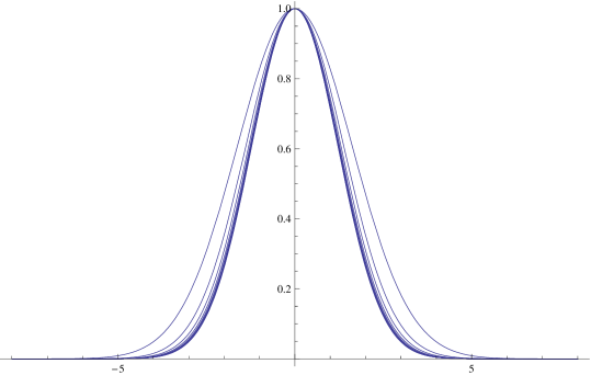
Figure 2.1: Fourier transform of the contraction $\langle\tilde{\Omega}^{L},:e^{ikX}:\rangle$ for the Witten deformation at $u=1$, plotted for $L=1,...,10$. The profiles are Gaussians $e^{-x^{2}/\Delta}$ which become localized up to a minimum width $\Delta\approx 1.46$ for large $L$. In this plot we have normalized the height of the Gaussians to $1$. Calculating the absolute normalization in our approach requires evaluating the trace of infinite dimensional matrices which are only known numerically, and convergence is unfortunately too slow to obtain acceptable accuracy, especially for large $L$. However, our numerics indicates that the normalization is finite and nonzero for $L\to\infty$.

3 The BMT and Ellwood Solutions

Ellwood’s original proposal for the lump solution[1] is given by writing the Schnabl gauge marginal solution[18, 19] as a formal gauge transformation of the tachyon vacuum, and then relaxing the assumption of marginality of the matter operator inside the gauge parameter. Extending this construction to dressed Schnabl gauges[15] yields a class of solutions of the form

$$\Phi_{f,g}=f\left(c\phi-\frac{1}{K+\phi}\phi^{\prime}\partial c\right)\frac{1}{1+\frac{1-fg}{K}\phi}\,Bc\,g.$$ (3.1)

We will call these Ellwood solutions. They are conjectured to be solutions in a string field theory formulated around $\mathrm{BCFT}_{0}$ which describe the endpoint of an RG flow triggered by $\phi(s)$, $\mathrm{BCFT}^{*}$. The string fields $f$ and $g$ (subject to a few conditions) can be any elements of the algebra of wedge states. Ellwood’s original solution corresponds to choosing $f$ and $g$ to be the square root of the $SL(2,\mathbb{R})$ vacuum. The motivation behind this proposal is a long story, discussed in depth in [1]; essentially it amounts to a formal argument that the solution should support the correct cohomology of open string states. Further evidence in favor of (3.1) was provided by BMT, who showed (in the special case $f=g=1$) that it has the correct coupling to closed string states[2]. Note that (3.1) assumes the existence of an inverse for $K+\phi$. This factor contains most of the physics of the solution, and, paradoxically, also the source of its difficulties.

In a few special cases (3.1) reduces to known solutions. If $\phi$ is a marginal operator (with nonsingular OPE), $\phi^{\prime}$ vanishes and (3.1) reduces to the dressed Schnabl gauge marginal solution[23]. Choosing $\phi=\phi^{\prime}=1$ gives the dressed Schnabl gauge tachyon vacuum solution[9].

The BMT solution[2] is a special case of (3.1) with $f=g=1$:

$$\Phi=c\phi-B\frac{1}{K+\phi}\phi^{\prime}c\partial c.$$ (3.2)

This is by far the simplest solution in the class (3.1). However, the presence of the identity-like term $c\phi$ means the BMT solution is more singular than other Ellwood solutions. However, it is not more singular in a sense which is important for the calculation of observables. For most of this paper (except section 5) we will study the BMT solution as a prototypical example. The general Ellwood solution can be obtained from the BMT solution by a transformation discovered by Zeze

$$Z_{f,g}[\Phi]=f\Phi\frac{1}{1+A\Phi}g,$$ (3.3)

where $A=\frac{1-fg}{K}B$. The Zeze map is a gauge transformation only on-shell.

The crucial ingredient in the solution is the definition of $\frac{1}{K+\phi}$. We will follow BMT and define it (via the Schwinger parameterization) as an integral over all deformed wedge states:

$$\frac{1}{K+\phi}=\int_{0}^{\infty}dt\,\tilde{\Omega}^{t}.$$ (3.4)

This integral converges only if the deformed sliver state $\tilde{\Omega}^{\infty}$ vanishes. However, keeping in mind condition 3), we would not expect the deformed sliver to vanish unless the solution describes the tachyon vacuum. Therefore, in interesting examples, the integral (3.4) is divergent. We can regulate this divergence, but there is another, more serious problem: Except for tachyon vacuum solutions, the integral (3.4) does not invert $K+\phi$,

$$(K+\phi)\left(\int_{0}^{\infty}dt\,\tilde{\Omega}^{t}\right)=-\int_{0}^{\infty}dt\frac{d}{dt}\tilde{\Omega}^{t}=1-\tilde{\Omega}^{\infty},$$ (3.5)

so the definition (3.4) does not accomplish its intended purpose. This means that if we substitute (3.4) in place of $\frac{1}{K+\phi}$, the BMT and Ellwood solutions will not satisfy the equations of motion.

We can ask whether it is possible to regulate the solution so as to restore the equations of motion. One way to do this is to replace $\phi$ with $\phi+\epsilon$ for $\epsilon>0$ (and therefore $\phi^{\prime}$ with $\phi^{\prime}+\epsilon$), which automatically regulates the Schwinger integral by exponentially suppressing the $t=\infty$ boundary of moduli space. The expression

$$\Psi_{\mathrm{tv}}(\epsilon)=c(\phi+\epsilon)-B\frac{1}{K+\phi+\epsilon}(\phi^{\prime}+\epsilon)c\partial c$$ (3.6)

is a solution to the equations of motion for all $\epsilon>0$, since $\phi+\epsilon$ is simply another choice of $\phi$. Unfortunately, this regularization drastically alters the physical interpretation of the solution: For all $\epsilon>0$, this is a (non universal) solution for the tachyon vacuum. To see this, note that the boundary interaction of $\phi(s)+\epsilon$ on a very large cylinder vanishes (assuming $\phi(s)$ is already tuned), thanks to the divergent integration of $\epsilon$ along the boundary.

Paradoxically, the unwanted sliver term in (3.5) which threatens the equations of motion is physically necessary. If it were possible to invert $K+\phi$, we could trivialize the cohomology around the BMT solution with the homotopy operator[2]

$$\frac{B}{K+\phi}.$$ (3.7)

Furthermore, the same mechanism which produces the unwanted boundary term also accounts for the correct IR coupling to closed string states[2]. Therefore in this setup there is a basic tension between the equations of motion and the desire to reproduce the physics of a nontrivial boundary conformal field theory in the infrared. This observation is already enough to exclude the BMT and Ellwood solutions as viable descriptions of the lump. Undoubtedly, another class of solutions, perhaps even closely related, can resolve this problem, but our goal in this paper is more narrow: We will show that, in spite of the failure of the equations of motion, the BMT and Ellwood solutions reproduce essentially all of the expected physics of the lump, when properly interpreted. The significance of this observation is currently unclear to us, but it seems potentially important.

Given that $\frac{1}{K+\phi}$ is divergent in the Fock space, one might worry that the BMT and Ellwood solutions are also divergent. Actually, this is not the case, because in (3.1) $\frac{1}{K+\phi}$ always appears multiplied by $B$, which annihilates the linear divergence proportional to the deformed sliver state ($B\tilde{\Omega}^{t}$ vanishes as $1/t^{3}$ for large $t$). As we will see, this cancellation is not enough to restore the equations of motion. In fact, it is in a sense accidental. There are other solutions which are in principle equivalent to Ellwood and BMT but actually diverge in the Fock space. Consider for example the solution

$$\hat{\Phi}=c\phi-\frac{1}{2}B\frac{1}{K+\phi}\phi^{\prime}c\partial c-\frac{1}{2}\phi^{\prime}c\partial c\frac{1}{K+\phi}B+\frac{1}{4}B\frac{1}{K+\phi}\phi^{\prime}\partial c\frac{1}{K+\phi}\phi^{\prime}\partial c\frac{1}{K+\phi},$$

which, unlike (3.1), satisfies the string field reality condition. Regulating $\frac{1}{K+\phi}$ with a cutoff, one can easily show that this expression has the correct coupling to closed string states. Nevertheless, unless $\phi$ triggers an RG flow to the tachyon vacuum, this solution diverges in the Fock space since the last term has too many powers of $\frac{1}{K+\phi}$. At present we do not know of any solution describing a nontrivial $\mathrm{BCFT}^{*}$ which is both real and finite.

4 BMT solution

4.1 Regularization and Closed String Overlap

The BMT and Ellwood solutions (3.2) and (3.1) are not well-defined string fields as they stand (except when they describe the tachyon vacuum), and to give them meaning we must apply some regularization. Implicitly the computations of [2] regulate by imposing a hard cutoff for the Schwinger integral (3.4). However, a finite cutoff is cumbersome for most calculations. Instead, we will consider the BMT solution as the $\epsilon\to 0$ limit of the string field

$$\Phi(\epsilon)=c\phi-B\frac{1}{K+\phi+\epsilon}\phi^{\prime}c\partial c,$$ (4.1)

where

$$\frac{1}{K+\phi+\epsilon}=\int_{0}^{\infty}dt\,e^{-\epsilon t}\tilde{\Omega}^{t}.$$ (4.2)

Here $\epsilon$ regulates the Schwinger integral by exponentially suppressing the $t=\infty$ boundary of moduli space. Therefore (4.1) is a finite, well-defined string field for all $\epsilon>0$. We will discuss the regularization of Ellwood solutions in section 5.

The nice thing about the regularization (4.1) is that $\Phi(\epsilon)$ can be neatly separated into two terms: the tachyon vacuum solution $\Psi_{\mathrm{tv}}(\epsilon)$ in (3.6), and a term $\Delta(\epsilon)$ which “builds” the lump on top of the tachyon vacuum:

$$\Phi(\epsilon)=\Psi_{\mathrm{tv}}(\epsilon)+\Delta(\epsilon),$$ (4.3)

where

$$\Delta(\epsilon)=-\epsilon c+B\frac{\epsilon}{K+\phi+\epsilon}c\partial c.$$ (4.4)

In the $\epsilon\to 0$ limit $\Delta(\epsilon)$ becomes a sliver-like state, but vanishes in the level expansion. Nevertheless it has a crucial effect on the calculation of observables. In this sense it is a kind of “phantom term.” Note the differing roles $\epsilon$ plays in (4.3). In $\Phi(\epsilon)$ it plays the role of a regulating parameter, but in $\Psi_{\mathrm{tv}}(\epsilon)$ it is a gauge parameter labeling a class of equivalent solutions for the tachyon vacuum.

Equation (4.3) is very useful for calculating observables, since it allows us to cleanly separate the “trivial” contribution from the tachyon vacuum from the physically interesting contribution of the lump. To illustrate this point, let us present an alternative computation of the closed string overlap, which was already computed in [2]. Recall from [25, 2] that the closed string overlap of the BMT solution should satisfy

$$\lim_{\epsilon\to 0}\mathop{\rm Tr}\nolimits[\mathcal{V}\,\Phi(\epsilon)]=-\mathcal{A}_{0}(\mathcal{V})+\mathcal{A}^{*}(\mathcal{V}),$$ (4.5)

where $\mathcal{A}_{0}(\mathcal{V})$ is the disk amplitude in $\mathrm{BCFT}_{0}$ with one on-shell closed string insertion $\mathcal{V}=c\tilde{c}\mathcal{V}^{\mathrm{m}}$, $\mathcal{A}^{*}(\mathcal{V})$ is the same quantity in $\mathrm{BCFT}^{*}$, and $\mathop{\rm Tr}\nolimits[\mathcal{V}\cdot]$ is the 1-string vertex with a midpoint insertion of $\mathcal{V}$. Plugging the regularized BMT solution into the right hand side of (4.5) we find two terms:

$$\mathop{\rm Tr}\nolimits[\mathcal{V}\,\Phi(\epsilon)]=\mathop{\rm Tr}\nolimits[\mathcal{V}\,\Psi_{\mathrm{tv}}(\epsilon)]+\mathop{\rm Tr}\nolimits[\mathcal{V}\,\Delta(\epsilon)].$$ (4.6)

The first term is the closed string overlap of a tachyon vacuum solution. Since the disk tadpole amplitude around the tachyon vacuum vanishes, the first term only contributes minus the disk amplitude around $\mathrm{BCFT}_{0}$. Therefore,

$$\mathop{\rm Tr}\nolimits[\mathcal{V}\,\Phi(\epsilon)]=-\mathcal{A}_{0}(\mathcal{V})+\mathop{\rm Tr}\nolimits[\mathcal{V}\,\Delta(\epsilon)].$$ (4.7)

Without any calculation we are already half-way done. The second term from $\Delta(\epsilon)$ must exclusively account for the nontrivial coupling between closed strings and $\mathrm{BCFT}^{*}$. Modulo ghost factors, we can already see that this is essentially guaranteed since $\Delta(\epsilon)$ is proportional to the deformed sliver state in the $\epsilon\to 0$ limit, and when we take the trace the boundary conditions are driven to the IR, producing the disk tadpole amplitude in $\mathrm{BCFT}^{*}$. Let us see this explicitly:

$$\mathop{\rm Tr}\nolimits[\mathcal{V}\,\Delta(\epsilon)]=\epsilon\int_{0}^{\infty}dt\,e^{-\epsilon t}\mathop{\rm Tr}\nolimits[\mathcal{V}\,\tilde{\Omega}^{t}Bc\partial c].$$ (4.8)

Simplifying the ghost correlator and substituting $\alpha=\epsilon t$ this becomes

$$\mathop{\rm Tr}\nolimits[\mathcal{V}\,\Delta(\epsilon)]=\int_{0}^{\infty}d\alpha\,e^{-\alpha}\left(-\,\frac{\epsilon}{\alpha}\mathop{\rm Tr}\nolimits[\mathcal{V}\,\tilde{\Omega}^{\alpha/\epsilon}c]\right).$$ (4.10)

The factor in the integrand can be written as a correlation function on the cylinder:

$$-\,\frac{\epsilon}{\alpha}\mathop{\rm Tr}\nolimits[\mathcal{V}\,\tilde{\Omega}^{\alpha/\epsilon}c]=-\left\langle\exp\left[\int_{0}^{\alpha/\epsilon}ds\,\phi(s)\right]\left(\frac{\alpha}{\epsilon}\right)\circ\Big{[}\mathcal{V}(i\infty)c(0)\Big{]}\right\rangle_{C_{\alpha/\epsilon}}.$$ (4.11)

In the $\epsilon\to 0$ limit the cylinder becomes very large, and the boundary conditions flow to the IR as described in condition 3). Thus,

$$\lim_{\epsilon\to 0}\left(-\,\frac{\epsilon}{\alpha}\mathop{\rm Tr}\nolimits[\mathcal{V}\,\tilde{\Omega}^{\alpha/\epsilon}c]\right)=-\langle\mathcal{V}(i\infty)c(0)\rangle_{C_{1}}^{\mathrm{BCFT}^{*}}.$$ (4.12)

The right hand side is precisely the amplitude for a single closed string to be emitted from the background $\mathrm{BCFT}^{*}$, as defined in the conventions of [25]. Integrating over $\alpha$ gives

$$\lim_{\epsilon\to 0}\mathop{\rm Tr}\nolimits[\mathcal{V}\,\Delta(\epsilon)]=\mathcal{A}^{*}(\mathcal{V}).$$ (4.13)

In total

$$\lim_{\epsilon\to 0}\mathop{\rm Tr}\nolimits[\mathcal{V}\,\Phi(\epsilon)]=-\mathcal{A}_{0}(\mathcal{V})+\mathcal{A}^{*}(\mathcal{V}),$$ (4.14)

as expected. Unlike the closed string overlap, the energy is a nonlinear function of the string field, and its separation into a tachyon vacuum and lump contribution is less obvious. We will see how this happens in section 4.3.

4.2 Anomaly in Equations of Motion

The regularization (4.1) does not produce a solution to the equations of motion, since, despite formal appearances, $\frac{1}{K+\phi+\epsilon}$ does not define an inverse for $K+\phi$ in the $\epsilon\to 0$ limit. We can check this:

$$(K+\phi)\frac{1}{K+\phi+\epsilon}=1-\frac{\epsilon}{K+\phi+\epsilon}.$$ (4.15)

The second term is not zero because the vanishing of $\epsilon$ is compensated by a linear divergence in $\frac{1}{K+\phi+\epsilon}$. To see what happens explicitly, plug in the Schwinger integral for $\frac{1}{K+\phi+\epsilon}$ and make a substitution $\alpha=\epsilon t$:

$$\frac{\epsilon}{K+\phi+\epsilon}=\int_{0}^{\infty}d\alpha\,e^{-\alpha}\tilde{\Omega}^{\alpha/\epsilon}.$$ (4.16)

Note that the overall factor of $\epsilon$ has disappeared. Taking $\epsilon\to 0$, the deformed wedge state in the integrand becomes the deformed sliver, independent of $\alpha$. Integration over $\alpha$ then produces a factor of 1 and we find

$$\lim_{\epsilon\to 0}(K+\phi)\frac{1}{K+\phi+\epsilon}=1-\tilde{\Omega}^{\infty},$$ (4.17)

exactly as we found in equation (3.5).

It is important to calculate precisely how the equations of motion fail. For this purpose, write the regularized BMT solution in the form

$$\Phi(\epsilon)=c\phi-A(\epsilon)\phi^{\prime}c\partial c,\ \ \ \ \ \ \ \ \ A(\epsilon)=\frac{B}{K+\phi+\epsilon},$$ (4.18)

where $A(\epsilon)$ is the homotopy operator which trivializes the cohomology around the tachyon vacuum solution $\Psi_{\mathrm{tv}}(\epsilon)$ in (3.6):

$$Q_{\Psi_{\mathrm{tv}}(\epsilon)}A(\epsilon)=1.$$ (4.19)

Now note from table 1 that the kinetic term of the equations of motion can be written

$$Q\Phi(\epsilon)=(1-QA(\epsilon))\phi^{\prime}c\partial c,$$ (4.20)

while the quadratic term can be written

$$\Phi(\epsilon)^{2}=-[\Phi(\epsilon),A(\epsilon)]\phi^{\prime}c\partial c.$$ (4.21)

The commutator of the right hand side is there for free, because the product of $\Phi(\epsilon)$ with $\phi^{\prime}c\partial c$ vanishes upon the collision of $c$s. Adding (4.20) and (4.21) together, we find

$$Q\Phi(\epsilon)+\Phi(\epsilon)^{2}=\Big{[}1-Q_{\Phi(\epsilon)}A(\epsilon)\Big{]}\phi^{\prime}c\partial c.$$ (4.22)

Therefore, the validity of the the equations of motion is directly related to question of whether the BMT solution supports open string states. If it does support open string states, then $Q_{\Phi(\epsilon)}A(\epsilon)$ cannot be $1$ since otherwise $A(\epsilon)$ would trivialize the cohomology. But then (4.22) implies the equations of motion cannot be satisfied.

Let us complete the computation of (4.22):

$$Q_{\Phi(\epsilon)}A(\epsilon)\!\!\!\!\!\!\!\! =Q_{\Psi_{\mathrm{tv}}(\epsilon)}A(\epsilon)+[\Delta(\epsilon),A(\epsilon)],$$ (4.23)

$$=1+[\Delta(\epsilon),A(\epsilon)].$$

The commutator is explicitly,

$$[\Delta(\epsilon),A(\epsilon)]=-cB\frac{\epsilon}{K+\phi+\epsilon}-\frac{\epsilon}{K+\phi+\epsilon}Bc+\frac{\epsilon}{K+\phi+\epsilon}\partial c\frac{B}{K+\phi+\epsilon}.$$ (4.24)

Now write $\partial c=[K+\phi+\epsilon,c]$. This allows us to cancel one of the inverse factors of $K+\phi+\epsilon$ in the third term, and adding up what remains gives simply

$$[\Delta(\epsilon),A(\epsilon)]=-\frac{\epsilon}{K+\phi+\epsilon}.$$ (4.25)

Therefore,

$$Q_{\Phi(\epsilon)}A(\epsilon)=1-\frac{\epsilon}{K+\phi+\epsilon},$$ (4.26)

and

$$Q\Phi(\epsilon)+\Phi(\epsilon)^{2}\!\!\!\!\!\!\!\! =\frac{\epsilon}{K+\phi+\epsilon}\phi^{\prime}c\partial c,$$ (4.27)

$$\equiv\Gamma(\epsilon),$$

where $\Gamma(\epsilon)$ is the anomaly in the equations of motion.

For $\epsilon>0$, the anomaly is (of course) nonzero, since $\Phi(\epsilon)$ is not intended to be a solution for nonzero $\epsilon$. In the limit $\epsilon\to 0$ we find

$$\Gamma(0)=\tilde{\Omega}^{\infty}\phi^{\prime}c\partial c.$$ (4.28)

In [2] it was implicitly assumed that this state vanishes. The intuition behind this expectation is that the deformed sliver tends to drive the boundary conditions to the IR, where $\phi^{\prime}$ vanishes by conformal invariance. Nevertheless, (4.28) is a nonvanishing state. The reason is because $\phi^{\prime}$ appears at the outer edge of the deformed sliver, where test states do not see the boundary conditions as conformal. More formally, since $\phi^{\prime}$ is on the edge it can have contractions with nearby operators which do not vanish in the sliver limit, even though the 1-point function of $\phi^{\prime}$ does vanish.

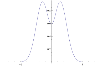
Figure 4.1: Fourier transform of the contraction $\langle\Gamma(0),c\!\!:\!\!e^{ikX}\!\!:\rangle$ assuming the Witten deformation at $u=1$. We were not able to accurately determine the normalization, but we believe it is finite and nonzero. We are not certain whether the double peak profile has a useful interpretation, though it is interesting to note that the equations of motion appear to be satisfied far away from the center of the lump. Perhaps not coincidentally, far away from the position of the brane we expect the solution to approximate the tachyon vacuum.

For the Witten deformation, we have calculated the overlap of $\Gamma(0)$ with a plane wave, giving the position space profile shown in figure 4.1. However, it is possible to see that the anomaly is nonvanishing with a simpler calculation. For the Witten deformation, consider a test state

$$\chi=\tilde{\Omega}^{1/2}(:\!X^{2}\!:\!\partial^{2}c)\tilde{\Omega}^{1/2},$$ (4.29)

where the strips on either side of the insertion are deformed. Contracting this with $\Gamma(0)$ gives a correlator whose entire boundary shares the same nonconformal boundary condition, and we can compute the correlator using formulas originally written down by Witten[14], reviewed in appendix A. The result is

$$\langle\Gamma(0),\chi\rangle=-16u\Big{[}\cos(2\pi u)\mathrm{ci}(2\pi u)+\sin(2\pi u)\mathrm{si}(2\pi u)\Big{]}^{2},$$ (4.30)

where $u$ is the boundary coupling of the Witten deformation and $\mathrm{ci}$ and $\mathrm{si}$ are the sine and cosine integrals

$$\mathrm{ci}(x)=-\int_{x}^{\infty}ds\frac{\cos s}{s}\ \ \ \ \ \ \ \ \mathrm{si}(x)=-\int_{x}^{\infty}ds\frac{\sin s}{s}.$$ (4.31)

We plot this as a function $u$ in figure 4.2. Note that the overlap vanishes for very large $u$:

$$\langle\Gamma(0),\chi\rangle\sim-\frac{1}{\pi^{4}u^{3}}\ \ \ (\mathrm{large}\ u).$$ (4.32)

This suggests that there is a sense in which the equations of motion are satisfied when formulating the solution directly at the infrared fixed point of the RG flow. We will say more about this when discussing the cohomology.

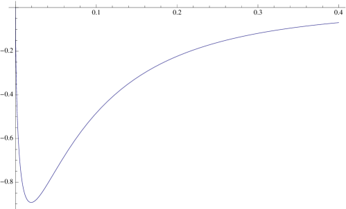
Figure 4.2: Anomaly in the equations of motion contracted with the state (4.29), plotted as a function of the boundary coupling $u$ of the Witten deformation (2.8) for $0<u<.4$.

4.3 Energy

Leaving the equations of motion to the side for a moment, let us proceed to calculate the energy of the BMT solution. For static backgrounds, we can calculate the energy by evaluating the action, and the result should be[2]

$$E=-S=\frac{1}{2\pi^{2}}(-g(0)+g(\infty)),$$ (4.33)

where $g(0)$ is the norm of the $SL(2,\mathbb{R})$ vacuum in $\mathrm{BCFT}_{0}$ and $g(\infty)$ is the norm of the $SL(2,\mathbb{R})$ vacuum in $\mathrm{BCFT}^{*}$. Note that $g(0)$ and $g(\infty)$ are related via RG flow of the disk partition function

$$g(L)=\mathop{\rm Tr}\nolimits[\tilde{\Omega}^{L}]^{m},$$ (4.34)

where $\mathop{\rm Tr}\nolimits[\cdot]^{m}$ is the trace in the matter component of $\mathrm{BCFT}_{0}$.

Since the equations of motion are not satisfied, there is no reason to expect to find the correct energy by computing the kinetic or cubic terms alone. Therefore, we will calculate the full gauge invariant action

$$S=\mathop{\rm Tr}\nolimits\left[-\frac{1}{2}\Phi(\epsilon)Q\Phi(\epsilon)-\frac{1}{3}\Phi(\epsilon)^{3}\right].$$ (4.35)

in the limit $\epsilon\to 0$.

Keeping track of the anomaly in the equations of motion, we can write the action

$$S=\mathop{\rm Tr}\nolimits\left[\frac{1}{6}\Phi(\epsilon)^{3}-\frac{1}{2}\Phi(\epsilon)\Gamma(\epsilon)\right].$$ (4.36)

Our strategy is to use the decomposition

$$\Phi(\epsilon)=\Psi_{\mathrm{tv}}(\epsilon)+\Delta(\epsilon)$$ (4.37)

to separate the action into a contribution from the tachyon vacuum and a contribution from the lump. We start by substituting this decomposition into the $\Phi(\epsilon)^{3}$ term:

$$S\!\!\!\!\!\!\!\! =\mathop{\rm Tr}\nolimits\left[\frac{1}{6}(\Psi_{\mathrm{tv}}(\epsilon)+\Delta(\epsilon))^{3}-\frac{1}{2}\Phi(\epsilon)\Gamma(\epsilon)\right],$$ (4.38)

$$=\mathop{\rm Tr}\nolimits\left[\frac{1}{6}\Psi_{\mathrm{tv}}(\epsilon)^{3}+\frac{1}{2}\Delta(\epsilon)\Psi_{\mathrm{tv}}(\epsilon)^{2}+\frac{1}{2}\Delta(\epsilon)^{2}\Psi_{\mathrm{tv}}(\epsilon)+\frac{1}{6}\Delta(\epsilon)^{3}-\frac{1}{2}\Phi(\epsilon)\Gamma(\epsilon)\right].$$

Now write the last four terms back in terms of $\Phi(\epsilon)$, keeping the $\Psi_{\mathrm{tv}}(\epsilon)^{3}$ term:

$$S=\mathop{\rm Tr}\nolimits\left[\frac{1}{6}\Psi_{\mathrm{tv}}(\epsilon)^{3}\right]+\mathop{\rm Tr}\nolimits\left[\frac{1}{2}\Delta(\epsilon)\Phi(\epsilon)^{2}-\frac{1}{2}\Delta(\epsilon)^{2}\Phi(\epsilon)+\frac{1}{6}\Delta(\epsilon)^{3}-\frac{1}{2}\Phi(\epsilon)\Gamma(\epsilon)\right].$$ (4.39)

The first term is the gauge invariant action evaluated on a solution for the tachyon vacuum. Without any calculation, we know what this quantity is: it is the vacuum energy of the reference $\mathrm{BCFT}_{0}$:

$$\frac{1}{6}\mathop{\rm Tr}\nolimits[\Psi_{\mathrm{tv}}(\epsilon)^{3}]=\frac{1}{2\pi^{2}}g(0).$$ (4.40)

We will take this equation as given. We do not have a general proof except to note that $\Psi_{\mathrm{tv}}(\epsilon)$ is related to other solutions for the tachyon vacuum, whose energy has been computed analytically, by gauge transformations which we believe are nonsingular and can be continuously deformed to the identity. For the Witten deformation we are able to verify (4.40) numerically, as discussed in appendix B.

Assuming (4.40), all we have to do is show that the four remaining terms in (4.39) conspire to give the energy of the lump. To simplify, we use the identity

$$\Delta(\epsilon)\Phi(\epsilon)=\Gamma(\epsilon).$$ (4.41)

This equality is easy to verify using the relations of table 1, though we don’t have an interpretation of why it holds. There does not seem to be an analogous relation for Ellwood solutions. At any rate, plugging (4.41) into (4.39), the term with the anomaly contracted with the solution cancels, and we are left with

$$S=\frac{1}{2\pi^{2}}g(0)+\mathop{\rm Tr}\nolimits\left[-\frac{1}{2}\Delta(\epsilon)\Gamma(\epsilon)+\frac{1}{6}\Delta(\epsilon)^{3}\right].$$ (4.42)

On the right hand side, both terms in the trace are sliver-like, and so they drive the boundary conditions to the IR. The term with the anomaly however has an insertion of $\phi^{\prime}$, which tends to kill the correlator as the boundary conditions become conformal. Therefore we can anticipate that only the $\Delta(\epsilon)^{3}$ term contributes to the energy of the lump. This is exactly as we would expect if $\Delta(\epsilon)$ were a genuine solution of the equations of motion for the lump expanded around the tachyon vacuum. However, as we know from previous discussion, it is not.

We now compute the right hand side of (4.42) explicitly. Start with the term

$$\mathop{\rm Tr}\nolimits[\Delta(\epsilon)\Gamma(\epsilon)]\!\!\!\!\!\!\!\! =\mathop{\rm Tr}\nolimits\left[\frac{\epsilon}{K+\phi+\epsilon}Bc\partial c\frac{\epsilon}{K+\phi+\epsilon}\phi^{\prime}c\partial c\right].$$ (4.43)

Expanding out the Schwinger integrals, making a change of variables, and separating the trace into matter and ghost components gives the expression

$$\mathop{\rm Tr}\nolimits[\Delta(\epsilon)\Gamma(\epsilon)]=\frac{1}{\epsilon}\int_{0}^{\infty}d\alpha\,\alpha^{2}e^{-\alpha}\mathop{\rm Tr}\nolimits[\tilde{\Omega}^{\alpha/\epsilon}\phi^{\prime}]^{m}\int_{0}^{1}dq\mathop{\rm Tr}\nolimits[\Omega^{1-q}Bc\partial c\Omega^{q}c\partial c]^{gh}.$$ (4.44)

Evaluating the ghost integral,

$$\mathop{\rm Tr}\nolimits[\Delta(\epsilon)\Gamma(\epsilon)]=-\frac{1}{2\pi^{2}}\frac{1}{\epsilon}\int_{0}^{\infty}d\alpha\,\alpha^{2}e^{-\alpha}\mathop{\rm Tr}\nolimits[\tilde{\Omega}^{\alpha/\epsilon}\phi^{\prime}]^{m}.$$ (4.45)

To get rid of the $\phi^{\prime}$ use the relation

$$\mathop{\rm Tr}\nolimits[\tilde{\Omega}^{L}\phi^{\prime}]^{m}=-\frac{d}{dL}g(L).$$ (4.47)

Note that this implies that the 1-point function of $\phi^{\prime}$ on a very large cylinder vanishes, since the disk partition function approaches a constant in the infrared (the IR norm of the $SL(2,\mathbb{R})$ vacuum). This is the sense in which the anomaly was naively expected to vanish. Plugging (4.47) into (4.46) we find

$$\mathop{\rm Tr}\nolimits[\Delta(\epsilon)\Gamma(\epsilon)]=-\frac{1}{2\pi^{2}}\int_{0}^{\infty}d\alpha\,\alpha e^{-\alpha}\left.\left[L\frac{d}{dL}g(L)\right]\right|_{L=\alpha/\epsilon}.$$ (4.48)

Since $g(L)$ approaches a constant its derivative must vanish faster than $1/L$. Therefore

$$\lim_{\epsilon\to 0}\mathop{\rm Tr}\nolimits[\Delta(\epsilon)\Gamma(\epsilon)]=0.$$ (4.49)

From the perspective of the gauge invariant action, the anomaly in the equations of motion vanishes.

Finally, compute the term

$$\frac{1}{6}\mathop{\rm Tr}\nolimits[\Delta(\epsilon)^{3}]=\frac{1}{6}\mathop{\rm Tr}\nolimits\left[\left(\frac{\epsilon}{K+\phi+\epsilon}Bc\partial c\right)^{3}\right].$$ (4.50)

Expanding the Schwinger integrals, and making a change of variables, and separating into matter/ghost components,

$$\frac{1}{6}\mathop{\rm Tr}\nolimits[\Delta(\epsilon)^{3}]=\frac{1}{6}\int_{0}^{\infty}d\alpha\,\alpha^{2}e^{-\alpha}g\left({\textstyle\frac{\alpha}{\epsilon}}\right)\int_{0}^{1}dq\int_{0}^{q}dr\mathop{\rm Tr}\nolimits[\Omega^{1-q}Bc\partial c\Omega^{q-r}Bc\partial c\Omega^{r}Bc\partial c]^{gh}.$$ (4.51)

Evaluating the ghost integral

$$\int_{0}^{1}dq\int_{0}^{q}dr\mathop{\rm Tr}\nolimits[\Omega^{1-q}Bc\partial c\Omega^{q-r}Bc\partial c\Omega^{r}Bc\partial c]^{gh}=-\frac{3}{2\pi^{2}}$$ (4.52)

gives

$$\frac{1}{6}\mathop{\rm Tr}\nolimits[\Delta(\epsilon)^{3}]=-\frac{1}{4\pi^{2}}\int_{0}^{\infty}d\alpha\,\alpha^{2}e^{-\alpha}g\left({\textstyle\frac{\alpha}{\epsilon}}\right).$$ (4.53)

In the $\epsilon\to 0$ limit the disk partition function becomes the norm of the $SL(2,\mathbb{R})$ vacuum in the infrared, and the integration over $\alpha$ gives a factor of $2!$. Thus

$$\lim_{\epsilon\to 0}\frac{1}{6}\mathop{\rm Tr}\nolimits[\Delta(\epsilon)^{3}]=-\frac{1}{2\pi^{2}}g(\infty).$$ (4.54)

and the total energy is

$$E=-S=\frac{1}{2\pi^{2}}(-g(0)+g(\infty)),$$ (4.55)

as expected.

We may ask how this result depends on our choice of regularization. It depends to some degree, since the tachyon vacuum solution (3.6) can be viewed as a regularization of the BMT solution. That being said, we believe that the lump energy works for a large class of regularizations of the BMT solution. For example, with an assumption, the energy works for any regularization which represents $\frac{1}{K+\phi}$ as a limit of states in the deformed wedge algebra while leaving the rest of the solution unchanged. This includes, for example, regulating the solution with a hard cutoff for the upper limit of the Schwinger integral (3.4). Nevertheless, the regularization we have used produces highly nontrivial simplifications which may have a deeper explanation.

4.4 Equations of Motion Contracted with the Solution

It is interesting to ask whether we would have obtained the correct energy calculating only the cubic or kinetic terms of the action. The answer to this question depends on whether the anomaly contracted with the solution,

$$\lim_{\epsilon\to 0}\mathop{\rm Tr}\nolimits[\Phi(\epsilon)\Gamma(\epsilon)],$$ (4.56)

vanishes. We see no reason why this quantity should vanish in general, but its explicit computation depends on the choice of relevant deformation and, since it is not gauge invariant, the particular form of the BMT solution. Here we compute (4.56) using the Witten deformation.

Plugging in the anomaly and BMT solution gives

$$\mathop{\rm Tr}\nolimits[\Phi(\epsilon)\Gamma(\epsilon)]\!\!\!\!\!\!\!\! =-\mathop{\rm Tr}\nolimits\left[\frac{B}{K+\phi+\epsilon}\phi^{\prime}c\partial c\frac{\epsilon}{K+\phi+\epsilon}\phi^{\prime}c\partial c\right].$$ (4.57)

Now on the right hand side we expand the Schwinger integrals and separate them into an integration over the total width of the cylinder and an integration over the relative positions of the $\phi^{\prime}c\partial c$ insertions within a cylinder of fixed width. In the $\epsilon\to 0$ limit only a cylinder with infinite circumference contributes to the integral, and we are left only with the integral over the separation of the $\phi^{\prime}c\partial c$ insertions:

$$\lim_{\epsilon\to 0}\mathop{\rm Tr}\nolimits[\Phi(\epsilon)\Gamma(\epsilon)]=-\lim_{L\to\infty}\left(L\int_{0}^{1}dq\,\mathop{\rm Tr}\nolimits[B\tilde{\Omega}^{Lq}\,\phi^{\prime}c\partial c\,\tilde{\Omega}^{L(1-q)}\,\phi^{\prime}c\partial c]\right).$$ (4.58)

The integration variable $q$ is the ratio between the circumference of the cylinder and the separation between the $\phi^{\prime}c\partial c$ insertions. To go further we need to evaluate the matter correlator, which requires us to specialize to the Witten deformation. The 2-point function of $\phi^{\prime}$ in the presence of the Witten boundary interaction can be easily computed from (A.14) in appendix A. Dropping the contribution from the square of the 1-point function of $\phi^{\prime}$, which vanishes as $1/L^{4}$, and computing the ghost correlator leaves the integral

$$\lim_{\epsilon\to 0}\mathop{\rm Tr}\nolimits[\Phi(\epsilon)\Gamma(\epsilon)]=-\frac{g(\infty)}{2\pi^{2}}\lim_{L\to\infty}\left(L^{2}\int_{0}^{1}dq\,\Big{[}\pi(1-q)\sin 2\pi q+\cos 2\pi q-1\Big{]}G(Lq,L)^{2}\right),$$ (4.59)

where $G(s,L)$ is the boundary Green’s function for the Witten deformation of two $X$ insertions separated by a distance $s$ on a cylinder of circumference $L$:

$$\left\langle e^{-\int_{0}^{L}dt\,\phi_{u}(t)}X(s)X(0)\right\rangle_{C_{L}}^{\mathrm{BCFT}_{0}}=g(L)G(s,L).$$ (4.60)

Its explicit form is given in (A.10). For generic $q$ the Green’s function in the integrand vanishes for large $L$, because the boundary conditions on a very large cylinder are effectively Dirichlet which forces $X=0$. The integral therefore can only receive contribution from singular contractions between two $X$s in the vicinity of $q=0$ and $q=1$. Furthermore, at $q=1$ the singular contraction between the $X$s is suppressed by a vanishing contraction between the pair of $c\partial c$s. Therefore, in the large $L$ limit the integral only receives contribution from the vicinity of $q=0$. To clearly extract this contribution, we make a substitution of variables $x=2\pi Lq$:

$$\lim_{\epsilon\to 0}\mathop{\rm Tr}\nolimits[\Phi(\epsilon)\Gamma(\epsilon)]=-\frac{g(\infty)}{4\pi^{2}}\lim_{L\to\infty}\left(L\int_{0}^{2\pi L}dx\,\frac{1}{\pi}\left[\pi\left(1-\frac{x}{2\pi L}\right)\sin\frac{x}{L}+\cos\frac{x}{L}-1\right]G\left(\frac{x}{2\pi},L\right)^{2}\right).$$ (4.61)

Making a series expansion of the trigonometric factor in the integrand, the integral further simplifies

$$\lim_{\epsilon\to 0}\mathop{\rm Tr}\nolimits[\Phi(\epsilon)\Gamma(\epsilon)]=-\frac{g(\infty)}{4\pi^{2}}\int_{0}^{\infty}dx\,x\,\lim_{L\to\infty}G\left(\frac{x}{2\pi},L\right)^{2}.$$ (4.62)

Thus we need to know the 2-point function of $X$s with fixed separation on a very large cylinder. This limit is given in (A.18). Thus the equations of motion contracted with the solution is

$$\lim_{\epsilon\to 0}\mathop{\rm Tr}\nolimits[\Phi(\epsilon)\Gamma(\epsilon)]=-\frac{g(\infty)}{\pi^{2}}w,$$ (4.63)

where $w$ is the value of the integral

$$w=\int_{0}^{\infty}dx\,x(\cos(x)\,\mathrm{ci}(x)+\sin(x)\mathrm{si}(x))^{2}=0.36685.$$ (4.64)

This means that if we had evaluated the cubic term in the action expecting to find the correct energy, instead we would have found

$$-\lim_{\epsilon\to 0}\frac{1}{6}\mathop{\rm Tr}\nolimits[\Phi(\epsilon)^{3}]\!\!\!\!\!\!\!\! =E-\frac{1}{2}\lim_{\epsilon\to 0}\mathop{\rm Tr}\nolimits[\Phi(\epsilon)\Gamma(\epsilon)]$$ (4.65)

$$=\frac{1}{2\pi^{2}}\Big{[}-g(0)+(1+w)g(\infty)\Big{]}.$$

which is incorrect.

5 Ellwood Solutions

5.1 Regularization

So far we have focused our analysis on the BMT solution. In a sense, the BMT solution is a degenerate example of Ellwood’s more general construction, and it is important to understand how much our analysis depends on accidental simplifications or singularities of this particular example.

Therefore in this section we study Ellwood solutions. The first question which arises is how the Ellwood solutions should be regularized. One obvious approach is to define the regulated Ellwood solution as a gauge transformation of the regulated BMT solution (4.1), by some off-shell extension of the Zeze map (3.3). However, this approach leads to regularizations which seem artificial, and it does not give any independent confirmation of the physics behind the BMT solution. Furthermore, one of the most important properties of Ellwood solutions is that they are (in general) much less singular than the BMT solution from the perspective of the identity string field. However, any gauge transformation of the BMT solution produces a state which is essentially as identity-like as the BMT solution.

Therefore we search for a way to regulate Ellwood solutions directly. Compared to BMT, where the physics of the solution appears to be reasonably independent of the choice of regularization, the regularization of Ellwood solutions is delicate. Many natural proposals turn out to be unphysical. We study one particular regularization which works: the $\epsilon\to 0$ limit of the string field

$$\Phi_{f,g}(\epsilon)=f\left[c\phi-\frac{1}{K+\phi+\epsilon}\phi^{\prime}\partial c\right]\frac{B}{1+\frac{1-fg}{K}(\phi+\epsilon)}cg.$$ (5.1)

Under reasonable assumptions about $f$ and $g$, this is a well-defined string field for all $\epsilon>0$. Like (4.1), this expression can be separated into a tachyon vacuum solution $\Psi^{\mathrm{tv}}_{f,g}(\epsilon)$ plus a term $\Delta_{f,g}(\epsilon)$ which “builds” the lump on top of the tachyon vacuum:

$$\Phi_{f,g}(\epsilon)=\Psi^{\mathrm{tv}}_{f,g}(\epsilon)+\Delta_{f,g}(\epsilon),$$ (5.2)

where

$$\Psi^{\mathrm{tv}}_{f,g}(\epsilon)\!\!\!\!\!\!\!\! =f\left[c(\phi+\epsilon)-\frac{1}{K+\phi+\epsilon}(\phi^{\prime}+\epsilon)\partial c\right]R(\epsilon)Bcg,$$

$$\Delta_{f,g}(\epsilon)\!\!\!\!\!\!\!\! =f\left[-\epsilon c+\frac{\epsilon}{K+\phi+\epsilon}\partial c\right]R(\epsilon)Bcg,$$ (5.3)

and for short we have defined the factor

$$R(\epsilon)\equiv\frac{1}{1+\frac{1-fg}{K}(\phi+\epsilon)}.$$ (5.4)

Note the extra $\epsilon$ in the denominator of the rightmost factor of (5.1). This $\epsilon$ plays no role in regulating the Schwinger integral, and if it was not there (5.1) would still be a well-defined string field for $\epsilon>0$. Nevertheless this $\epsilon$ turns out to be necessary to recover the correct physics in the infrared; it is not sufficient to only regulate the divergent Schwinger integral. Also note that (5.1) is not a gauge transformation of BMT. Therefore, to see the correct physics emerge in the infrared requires genuinely new calculations.

The Ellwood solution has the same problem with inverting $K+\phi$ as the BMT solution, so we would not expect it to satisfy the equations of motion. Computing the equations of motion from (5.1) we find

$$Q\Phi_{f,g}(\epsilon)+\Phi_{f,g}(\epsilon)^{2}=f\Big{[}\Gamma(\epsilon)-\Phi(\epsilon)\Delta(\epsilon)\Big{]}R(\epsilon)Bcg+\Big{[}f\Phi(\epsilon)R(\epsilon)Bcg\Big{]}\Big{[}f\Delta(\epsilon)R(\epsilon)Bcg\Big{]},$$ (5.5)

where $\Phi(\epsilon),\Delta(\epsilon)$, and $\Gamma(\epsilon)$ are defined in section 4. The anomaly is a complicated expression, and we will not attempt to calculate its overlap with test states. We do not expect it to vanish in the $\epsilon\to 0$ limit.

5.2 Overlap and Energy

We now show that the regularization (5.1) correctly captures the physics of the lump, just like the BMT solution.

We start by computing the closed string overlap:

$$\mathop{\rm Tr}\nolimits[\mathcal{V}\,\Phi_{f,g}(\epsilon)]\!\!\!\!\!\!\!\! =\mathop{\rm Tr}\nolimits[\mathcal{V}\,\Phi(\epsilon)R(\epsilon)Bc\,\omega]$$ (5.6)

$$=\mathop{\rm Tr}\nolimits[\mathcal{V}\,c\phi R(\epsilon)Bc\,\omega]-\mathop{\rm Tr}\nolimits\left[\mathcal{V}\,\frac{1}{K+\phi+\epsilon}\phi^{\prime}\partial cR(\epsilon)Bc\,\omega\right],$$

where $\omega\equiv fg$ for short. Now in the second term insert a trivial factor of $Bc$ next to the $\partial c$. This allows us to eliminate the $Bc$ between $R(\epsilon)$ and $\omega$ to find

$$\mathop{\rm Tr}\nolimits[\mathcal{V}\,\Phi_{f,g}(\epsilon)]=\mathop{\rm Tr}\nolimits[\mathcal{V}\,c\phi R(\epsilon)Bc\,\omega]-\mathop{\rm Tr}\nolimits\left[\mathcal{V}\,B\phi^{\prime}c\partial c\left(R(\epsilon)\,\omega\frac{1}{K+\phi+\epsilon}\right)\right].$$ (5.7)

The factor in parentheses on the right can be simplified in a useful way. To see how, we write $\omega$ in a particular form:

$$\omega\!\!\!\!\!\!\!\! =-\frac{1-\omega}{K}K+1,$$ (5.8)

$$=-\frac{1-\omega}{K}(K+\phi+\epsilon)+1+\frac{1-\omega}{K}(\phi+\epsilon),$$

$$=R(\epsilon)^{-1}-\frac{1-\omega}{K}(K+\phi+\epsilon).$$

Therefore

$$R(\epsilon)\,\omega\frac{1}{K+\phi+\epsilon}=\frac{1}{K+\phi+\epsilon}-R(\epsilon)\frac{1-\omega}{K}.$$ (5.9)

Plugging this into the parentheses of (5.6) the $\frac{1}{K+\phi+\epsilon}$ term above combines with the insertions to give the overlap of the regularized BMT solution. Keeping track of the other terms gives

$$\mathop{\rm Tr}\nolimits[\mathcal{V}\,\Phi_{f,g}(\epsilon)]=\mathop{\rm Tr}\nolimits[\mathcal{V}\,\Phi(\epsilon)]+\mathop{\rm Tr}\nolimits\Big{[}\mathcal{V}\,c\phi R(\epsilon)Bc\,\omega\Big{]}+\mathop{\rm Tr}\nolimits\left[\mathcal{V}\,B\phi^{\prime}c\partial cR(\epsilon)\frac{1-\omega}{K}\right].$$ (5.10)

The overlap of the BMT solution was already computed in section 4.1 and [2], and we know it gives the correct shift in the closed string tadpole. All we have to do is show that the last two terms cancel in the $\epsilon\to 0$ limit. This can be done with a few specially chosen manipulations:

$$\mathop{\rm Tr}\nolimits[\mathcal{V}\,\Phi_{f,g}(\epsilon)]-\mathop{\rm Tr}\nolimits[\mathcal{V}\,\Phi(\epsilon)]\!\!\!\!\!\!\!\! =\mathop{\rm Tr}\nolimits\left[\mathcal{V}\,R(\epsilon)Bc\left(\omega c\phi+B\frac{1-\omega}{K}\phi^{\prime}c\partial c\right)\right],$$ (5.11)

$$=-\mathop{\rm Tr}\nolimits\left[\mathcal{V}\,R(\epsilon)Bc\,Q\left(B\frac{1-\omega}{K}c\phi\right)\right].$$

Replace the $R(\epsilon)Bc$ factor in the trace by an equivalent expression dressed up with redundant factors of $Bc$:

$$\mathop{\rm Tr}\nolimits[\mathcal{V}\,\Phi_{f,g}(\epsilon)]-\mathop{\rm Tr}\nolimits[\mathcal{V}\,\Phi(\epsilon)]\!\!\!\!\!\!\!\! =-\mathop{\rm Tr}\nolimits\left[\mathcal{V}\,\frac{1}{1+B\frac{1-\omega}{K}c(\phi+\epsilon)}Q\left(B\frac{1-\omega}{K}c\phi\right)\right].$$ (5.12)

The right hand side is almost the overlap of a pure gauge solution. We just have to fix up the string field inside the BRST variation:

$$\mathop{\rm Tr}\nolimits[\mathcal{V}\,\Phi_{f,g}(\epsilon)]-\mathop{\rm Tr}\nolimits[\mathcal{V}\,\Phi(\epsilon)]\!\!\!\!\!\!\!\! =-\mathop{\rm Tr}\nolimits\left[\mathcal{V}\,\frac{1}{1+B\frac{1-\omega}{K}c(\phi+\epsilon)}Q\left(1+B\frac{1-\omega}{K}c(\phi+\epsilon)\right)\right],$$ (5.13)

$$\ \ \ \ \ \ +\epsilon\mathop{\rm Tr}\nolimits\left[\mathcal{V}\,R(\epsilon)Bc\,Q\left(B\frac{1-\omega}{K}c\right)\right].$$

The first term is the closed string overlap of a pure gauge solution. Assuming $R(\epsilon)$ admits a convergent geometric series expansion in powers of $\frac{1-\omega}{K}(\phi+\epsilon)$, this term can be shown to vanish order by order. Therefore only the second term contributes for finite $\epsilon$, giving

$$\mathop{\rm Tr}\nolimits[\mathcal{V}\,\Phi_{f,g}(\epsilon)]=\mathop{\rm Tr}\nolimits[\mathcal{V}\,\Phi(\epsilon)]+\epsilon\mathop{\rm Tr}\nolimits\left[\mathcal{V}\,R(\epsilon)Bc\,Q\left(B\frac{1-\omega}{K}c\right)\right].$$ (5.14)

The second term vanishes since the string field in the trace is regular in the $\epsilon\to 0$ limit. Therefore the Ellwood solutions (5.1) have precisely the correct coupling to closed string states.

The overlaps of the Ellwood and BMT solutions are not precisely equal for $\epsilon>0$ because the regularized Ellwood solution (5.1) is not a gauge transformation of the regularized BMT solution (4.1). However, one might think that the overlaps must be equal in the $\epsilon\to 0$ limit because the Ellwood and BMT solutions are (formally) gauge equivalent. Actually, this is not the case. Many other regularizations of the Ellwood solution do not reproduce the correct coupling to closed strings. Consider what would happen if we had only regulated the Schwinger integral, and not included the extra $\epsilon$ in the rightmost factor of (5.1). In this case the regularized Ellwood solution would be

$$\Phi_{f,g}(\epsilon)=f\Phi(\epsilon)R(0)Bcg,$$ (5.15)

where $R(0)$ is (5.4) at $\epsilon=0$. The calculation of the overlap proceeds analogously, but, to extract the overlap of the regularized BMT solution, instead of (5.9) we need the relation

$$R(0)\,\omega\frac{1}{K+\phi+\epsilon}=\frac{1}{K+\phi+\epsilon}-R(0)\frac{1-\omega}{K}-R(0)\frac{1-\omega}{K}\frac{\epsilon}{K+\phi+\epsilon}.$$ (5.16)

The main difference between this and (5.9) is the third term. While the third term is proportional to $\epsilon$, it is nonvanishing in the $\epsilon\to 0$ limit, and actually gives the sole contribution to the difference between the Ellwood and BMT overlaps:

$$\mathop{\rm Tr}\nolimits[\mathcal{V}\,\Phi_{f,g}(\epsilon)]=\mathop{\rm Tr}\nolimits[\mathcal{V}\,\Phi(\epsilon)]+\mathop{\rm Tr}\nolimits\left[\mathcal{V}\,B\phi^{\prime}c\partial cR(0)\frac{1-\omega}{K}\frac{\epsilon}{K+\phi+\epsilon}\right].$$ (5.17)

In the $\epsilon\to 0$ limit the second term becomes

$$\mathop{\rm Tr}\nolimits\left[\mathcal{V}\,B\phi^{\prime}c\partial cR(0)\frac{1-\omega}{K}\tilde{\Omega}^{\infty}\right].$$ (5.18)

This does not appear to vanish for generic choice of $f$ and $g$. Therefore the fact that the closed string overlap works in (5.14) is not a consequence of a formal gauge equivalence, but is an independent confirmation of the physics behind the construction.

We can calculate the energy of the Ellwood solutions (5.1) by analogy with the BMT solution. The idea is to extract the negative energy from the tachyon vacuum, and to reduce the remaining terms to their BMT counterparts by repeated use of the identity (5.9). The calculation requires keeping track of many terms, and is too lengthy and mostly routine to be worth presenting here. Some aspects however deserve mention. The first is that for the Ellwood solutions (with this regularization) there is no simple relation between the anomaly, solution, and phantom term analogous to (4.41). This relation was crucial for simplifying the action from (4.39) to (4.42). For Ellwood solutions this simplification does not happen automatically, and the terms which would otherwise simplify have to be expanded and shown to cancel in a nontrivial fashion. The second point is that the calculation produces many spurious terms which do not cancel identically for $\epsilon>0$. Most of these terms are impractical to explicitly compute for $\epsilon>0$, and they must be argued to vanish for general reasons in the $\epsilon\to 0$ limit. These terms take one of three forms:

$$\epsilon\mathop{\rm Tr}\nolimits[X(\epsilon)],\ \ \ \ \ \ \epsilon\mathop{\rm Tr}\nolimits\left[X(\epsilon)\frac{\epsilon}{K+\phi+\epsilon}\right],\ \ \ \ \ \ \mathop{\rm Tr}\nolimits\left[X(\epsilon)B\frac{\epsilon}{K+\phi+\epsilon}\right],$$ (5.19)

where $X(\epsilon)$ is a finite and not sliver-like string field, generally some combination of $R(\epsilon),\ \omega,\ \frac{1-\omega}{K},\ \phi,\ \phi^{\prime}$, and ghosts. The first two classes of terms vanish because an overall factor $\epsilon$ multiplies a trace we believe is finite in the $\epsilon\to 0$ limit. The third class of terms vanish because in the $\epsilon\to 0$ limit the ghost component of the correlator has insertions with effectively positive scaling dimension on a very large cylinder. This is essentially the reasons why $B$ annihilates the sliver in the Fock space. With this understanding, the calculation of the energy is straightforward and reproduces the expected answer (4.55).

6 Cohomology?

It is interesting to ask whether the BMT solution supports the expected cohomology of open string states. Of course, taken literally this question has no meaningful answer, since the shifted kinetic operator is not nilpotent:

$$Q_{\Phi(\epsilon)}^{2}=[\Gamma(\epsilon),\cdot]$$ (6.1)

So the existence of cohomology is closely related to the equations of motion. In this section we argue that the BMT solution satisfies the equations of motion when contracted with states of the IR boundary conformal field theory, in a sense described below. Then, the BMT kinetic operator is nilpotent in $\mathrm{BCFT}^{*}$, and defines a cohomology.

As a first step, let us explain what it means to contract the equations of motion, which is a state in $\mathrm{BCFT}_{0}$, with states in $\mathrm{BCFT}^{*}$. Suppose

$$\Pi_{i}^{*}=\Omega^{1/2}\pi_{i}^{*}\Omega^{1/2}$$ (6.2)

are a basis of Fock states of $\mathrm{BCFT}^{*}$, where $\pi_{i}^{*}$ are vertex operators and (in this equation) $\Omega$ is the $SL(2,\mathbb{R})$ vacuum of $\mathrm{BCFT}^{*}$. This basis can be equivalently characterized in $\mathrm{BCFT}_{0}$ as a singular, projector-like limit of states of the form

$$\Pi_{i}(\epsilon)=\tilde{\Omega}^{1/2\epsilon}\pi_{i}(\epsilon)\tilde{\Omega}^{1/2\epsilon},$$ (6.3)

when $\epsilon\to 0$. The equivalence between $\Pi_{i}^{*}$ and $\Pi_{i}(\epsilon)$ can be explained as follows: In correlation functions on the cylinder, $\Pi_{i}(\epsilon)$ represents a strip of worldsheet of width $1/\epsilon$ with deformed boundary conditions and an operator $\pi_{i}(\epsilon)$ inserted in the middle. With a reparameterization, we can squeeze the strip to width $1$, whereupon the boundary conditions flow to $\mathrm{BCFT}^{*}$, and the operator $\pi_{i}(\epsilon)$, if appropriately chosen, flows to $\pi_{i}^{*}$. In particular, this means that $N$-string vertices of $\Pi_{i}(\epsilon)$, when $\epsilon\to 0$, are equal to the corresponding $N$-string vertices of $\Pi_{i}^{*}$, and so for string field theory purposes the states are indistinguishable.

With this understanding, the BMT solution satisfies the equations of motion in $\mathrm{BCFT}^{*}$ in the following sense:

$$\lim_{\epsilon\to 0}\Big{\langle}\Pi_{i}(\epsilon),\,Q\Phi(\epsilon)+\Phi(\epsilon)^{2}\Big{\rangle}=\lim_{\epsilon\to 0}\Big{\langle}\Pi_{i}(\epsilon),\Gamma(\epsilon)\Big{\rangle}=0.$$ (6.4)

To see why (6.4) holds, note that, because of the very large width of the test state $\Pi_{i}(\epsilon)$, contractions between $\phi^{\prime}$ and the vertex operator $\pi_{i}(\epsilon)$ are suppressed by cluster decomposition. Therefore (6.4) should be proportional to the one point function of $\phi^{\prime}$ on a very large (deformed) cylinder. This vanishes faster than $\epsilon$ because the disk partition function is constant in the infrared, by (4.47). The ghost correlator diverges as $\frac{1}{\epsilon}$, but this is not enough to cancel the vanishing matter correlator.

Let us clarify a possibly confusing point: (6.4) does not imply that the BMT solution is a well defined state in $\mathrm{BCFT}^{*}$ satisfying the equations of motion. In fact it is not: the overlap of $\Phi(\epsilon)$ with $\Pi_{i}(\epsilon)$ diverges in the $\epsilon\to 0$ limit. However, the anomaly in the equations of motion is a well-defined state in $\mathrm{BCFT}^{*}$, and it is precisely zero. This is all we need for the cohomology.

Acting within $\mathrm{BCFT}^{*}$, the BMT kinetic operator takes the form

$$\Big{\langle}\Pi_{i}(\epsilon),\,Q_{\Phi(\epsilon)}\Pi_{j}(\epsilon)\Big{\rangle}=\Big{\langle}\Pi_{i}(\epsilon),\,Q\Pi_{j}(\epsilon)+[\Phi(\epsilon),\Pi_{j}(\epsilon)]\Big{\rangle}.$$ (6.5)

Since the BMT solution is not well-defined in $\mathrm{BCFT}^{*}$, it is not obvious that the BMT kinetic operator should be meaningful either. To see what happens, concentrate first on the action of the BRST operator, $Q$. When $Q$ acts on a deformed wedge state, it can be naturally separated into two pieces:

$$Q=-[c\phi,\,\cdot\,]+\tilde{Q}.$$ (6.6)

If $\phi$ were a marginal operator, the first part would be the BRST variation of the boundary condition changing operator, and the second part, $\tilde{Q}$, would be the BRST operator of the marginally deformed boundary conformal field theory. Since $\phi$ is not marginal, $\tilde{Q}$ is not a BRST charge, and it is not nilpotent:

$$\tilde{Q}^{2}=[\phi^{\prime}c\partial c,\,\cdot\,].$$ (6.7)

However, the operator $\phi^{\prime}c\partial c$ vanishes in $\mathrm{BCFT}^{*}$ for the same reason that the anomaly vanishes. Therefore, in the $\epsilon\to 0$ limit $\tilde{Q}$ is nilpotent and can be naturally identified with the BRST operator of the infrared boundary conformal field theory:

$$\lim_{\epsilon\to 0}\langle\Pi_{i}(\epsilon),\tilde{Q}\Pi_{j}(\epsilon)\rangle=\langle\Pi_{i}^{*},Q\Pi_{j}^{*}\rangle.$$ (6.8)

The $-[c\phi,\cdot]$ term in the BRST operator diverges as $\epsilon\to 0$, but thankfully it cancels against the corresponding divergence from the BMT solution in (6.5). The remaining piece of the BMT solution, $-\frac{1}{K+\phi+\epsilon}B\phi^{\prime}c\partial c$, does not contribute in the $\epsilon\to 0$ limit because the $1$-point function of $\phi^{\prime}$ kills the matter correlator. Adding everything up gives the simple result:

$$\lim_{\epsilon\to 0}\Big{\langle}\Pi_{i}(\epsilon),Q_{\Phi(\epsilon)}\Pi_{j}(\epsilon)\Big{\rangle}=\langle\Pi_{i}^{*},Q\Pi_{j}^{*}\rangle.$$ (6.9)

Therefore the BMT kinetic operator in the infrared is the same as the BRST operator of $\mathrm{BCFT}^{*}$, and they share the same cohomology.

It is interesting to see how the cohomology disappears for the tachyon vacuum regularization of the BMT solution, $\Psi_{\mathrm{tv}}(\epsilon)$ in (3.6). Repeating the above steps, in the tachyon vacuum kinetic operator in the IR takes the form

$$\lim_{\epsilon\to 0}\Big{\langle}\Pi_{i}(\epsilon),Q_{\Psi_{\mathrm{tv}}(\epsilon)}\Pi_{j}(\epsilon)\Big{\rangle}=\langle\Pi_{i}^{*},Q\Pi_{j}^{*}\rangle-\lim_{\epsilon\to 0}\Big{\langle}\Pi_{i}(\epsilon),[\Delta(\epsilon),\Pi_{j}(\epsilon)]\Big{\rangle},$$ (6.10)

Performing a scale transformation of the second term, we can replace $\Pi_{i}(\epsilon)$ with $\Pi_{i}^{*}$ and $\Delta(\epsilon)$ with $-c+\frac{1}{K+1}Bc\partial c$, where “$K$” is now the $K$ of the IR boundary conformal field theory. Therefore

$$\lim_{\epsilon\to 0}\Big{\langle}\Pi_{i}(\epsilon),Q_{\Psi_{\mathrm{tv}}(\epsilon)}\Pi_{j}(\epsilon)\Big{\rangle}=\left\langle\Pi_{i}^{*},Q\Pi_{j}^{*}+\left[\frac{1}{K+1}(c+Q(Bc)),\Pi_{j}^{*}\right]\right\rangle.$$ (6.11)

The right hand side is precisely the kinetic operator of the “simple” tachyon vacuum solution described in [15]. Note that because

$$\lim_{\epsilon\to 0}\Big{\langle}\Pi_{i}(\epsilon),\Delta(\epsilon)\Big{\rangle}=-\left\langle\Pi_{i}^{*},\frac{1}{K+1}(c+Q(Bc))\right\rangle,$$ (6.12)

$\Delta(\epsilon)$ is a well defined state in $\mathrm{BCFT}^{*}$, and is precisely the perturbative vacuum of $\mathrm{BCFT}^{*}$ as seen from the tachyon vacuum. This is consistent with the interpretation of $\Delta(\epsilon)$ as “building” the lump on top of the tachyon vacuum.

7 Concluding Remarks

In this paper we studied a class of formal solutions which were conjectured to describe lower dimensional branes as tachyon lumps in open string field theory. We found that the solutions do not satisfy the equations of motion. Nevertheless, they have the correct coupling to closed string states, and evaluating the action gives the expected energy.

The current situation is puzzling since the correct solution remains to be found, yet clearly this construction is capturing the physics of the desired solution in a nontrivial fashion. The question now is how to proceed. We offer a few possibilities:

• It is possible that while the specific solutions (3.1) are problematic, other solutions within the subset of states generated by multiplying $K,B,c,\phi$, and $\phi^{\prime}$ could describe a tachyon lump. It is difficult to analyze the full set of candidate solutions in generality, but we have found that the difficulties with Ellwood’s proposal are fairly generic. Perhaps a novel mechanism selects a particular subclass of solutions for which the equations of motion can be made non-anomalous.

• It is possible that the Ellwood and BMT solutions satisfy the equations of motion when correctly defined, but we have not identified the necessary definition of expressions such as $\frac{1}{K+\phi}$ when they appear inside the solution. It is worth mentioning that analogous problems with defining $\frac{1}{K}$ appear when studying of multibrane solutions[27], and new developments on this front may also have implications for lump solutions.

• Finally, it is possible that the current setup is for some reason inadequate to capture nonsingular lump solutions. Perhaps a different approach, for example based on boundary condition changing operators, as suggested in [17], is needed.

We hope that the current work will stimulate further thought on this important problem.

Acknowledgments

We would like to thank the organizers of the conference SFT 2010 in Kyoto where this collaboration began, and Micheal Kiermaier , Yuji Okawa, and Martin Schnabl for useful conversations. We would like to thank L. Bonora for making his numerical computations available to us. We thank Ian Ellwood for comments on the second version of the paper. This research was supported by the EURYI grant GACR EYI/07/E010 from EUROHORC and ESF.

Appendix A Witten Deformation

In this appendix we give some formulas which allow for explicit computation of correlation functions on the cylinder in the presence of the Witten boundary interaction. Most of the formulas follow immediately from [14] with the appropriate transcription.

The Witten deformation is generated by inserting the operator

$$\exp\left[-\int_{0}^{L}ds\,\phi_{u}(s)\right]$$ (A.1)

into correlation functions on the cylinder in a reference $\mathrm{BCFT}_{0}$ which includes a noncompact free boson $X(z,\bar{z})$ subject to Neumann boundary conditions, where

$$\phi_{u}(s)=u\left[\frac{1}{2}:X(s)^{2}:+\gamma-1+\ln(2\pi u)\right]\\$$ (A.2)

and

$$\phi^{\prime}_{u}(s)=u\frac{d}{du}\phi_{u}(s)=\phi_{u}(s)+u.$$ (A.3)

Here $u$ is a parameter which we are free to choose. Different $u$s are related by the scale transformation (2.6). For short, let’s write

$$\langle...\rangle^{u}_{C_{L}}=\left\langle\exp\left[-\int_{0}^{L}ds\,\phi_{u}(s)\right]...\right\rangle_{C_{L}}^{\mathrm{BCFT}_{0}}.$$ (A.4)

The $X$ part of the worldsheet theory is Gaussian and therefore completely defined by the zero point and bulk 2-point functions

$$\langle 1\rangle^{u}_{C_{L}}\!\!\!\!\!\!\!\! =g(L)$$ (A.5)

$$\langle X(z_{1},\bar{z}_{1})X(z_{2},\bar{z}_{2})\rangle^{u}_{C_{L}}\!\!\!\!\!\!\!\! =g(L){\bf G}(z_{1},\bar{z_{1}};z_{2},\bar{z}_{2};L),$$ (A.6)

where, leaving the $u$ dependence implicit, $g(L)$ is the disk partition function and ${\bf G}$ is the bulk Green’s function:

$$g(L)\!\!\!\!\!\!\!\! =\sqrt{\frac{uL}{2\pi}}\left(\frac{e}{uL}\right)^{uL}\Gamma(uL)$$ (A.7)

$${\bf G}(z_{1},\bar{z_{1}};z_{2},\bar{z}_{2};L)\!\!\!\!\!\!\!\! =-\frac{1}{2}\left(\ln|Z_{1}-Z_{2}|^{2}-\ln|1-Z_{1}\bar{Z}_{2}|^{2}\right)$$ (A.8)

$$\ \ \ \ \ \ \ \ \ \ \ \ \ \ \ \ \ -\frac{1}{uL}+2\mathrm{Re}\big{[}\Phi(Z_{1}\bar{Z_{2}},1,uL)\big{]}\ \ \ \ \ \ \ \ (Z=e^{\frac{2\pi i}{L}z}),\ \ \ \ \ \ \ \$$

where $\Phi(z,s,a)$ is the Lerch zeta function

$$\Phi(z,s,a)=\sum_{k=0}^{\infty}\frac{z^{k}}{(k+a)^{s}}.$$ (A.9)

For most applications we are interested in computing $n$-point functions of $\phi_{u}(s)$. For this purpose it is helpful to define the boundary Green’s function and the normalized 1-point function:

$$G(s,L)\!\!\!\!\!\!\!\! =-\frac{1}{uL}+2\mathrm{Re}\left[\Phi\left(e^{\frac{2\pi i}{L}s},1,uL\right)\right],$$ (A.10)

$$W(L)\!\!\!\!\!\!\!\! =-u\left[1+\frac{1}{2uL}+\psi(uL)-\ln(uL)\right],$$ (A.11)

where $\psi$ is the digamma function. With these objects can write explicit expressions for the $0,1,2$ and $3$ point functions using Wick’s theorem:

$$\langle 1\rangle^{u}_{C_{L}}\!\!\!\!\!\!\!\! =g(L),$$ (A.12)

$$\langle\phi_{u}(s)\rangle^{u}_{C_{L}}\!\!\!\!\!\!\!\! =g(L)W(L),$$ (A.13)

$$\langle\phi_{u}(s_{1})\phi_{u}(s_{2})\rangle^{u}_{C_{L}}\!\!\!\!\!\!\!\! =g(L)\left[W(L)^{2}+\frac{u^{2}}{2}G(s_{12},L)^{2}\right],$$ (A.14)

$$\langle\phi_{u}(s_{1})\phi_{u}(s_{2})\phi_{u}(s_{3})\rangle^{u}_{C_{L}}\!\!\!\!\!\!\!\! =g(L)\left[W(L)^{3}+\frac{u^{2}}{2}W(L)\big{(}G(s_{12},L)^{2}+G(s_{23},L)^{2}+G(s_{31},L)^{2}\big{)}\right.$$ (A.15)

$$\ \ \ +u^{3}G(s_{12},L)G(s_{23},L)G(s_{31},L)\Big{]}.$$

We can write similar expressions for higher point functions as well, but we will not need them.

For computations related to the anomaly it is useful to have asymptotic formulas for the large $L$ behavior of these $n$-point functions. For this purpose we list some large $L$ expansions:

$$g(L)\!\!\!\!\!\!\!\! =1\,+\,\frac{1}{12}\frac{1}{uL}\,+\,\frac{1}{288}\frac{1}{(uL)^{2}}\,-\,\frac{139}{51840}\frac{1}{(uL)^{3}}+...$$ (A.16)

$$=\exp\left[\sum_{n=1}^{\infty}\frac{B_{2n}}{2n(2n-1)}\frac{1}{(uL)^{2n-1}}\right],$$

$$W(L)\!\!\!\!\!\!\!\! =-u\left[\,1\,-\,\frac{1}{12}\frac{1}{(uL)^{2}}\,+\,\frac{1}{120}\frac{1}{(uL)^{4}}\,-\,...\right]$$ (A.17)

$$=-u\left[1-\sum_{n=1}^{\infty}\frac{B_{2n}}{2n}\frac{1}{(uL)^{2n}}\right],$$

where $B_{n}$ are the Bernoulli numbers. For the boundary Green’s function we can derive an asymptotic expansion for large $L$ and fixed separation $s$ between the $X$ insertions:

$$G(s,L)=-2\Big{[}\cos(2\pi us)\mathrm{ci}(2\pi us)+\sin(2\pi us)\mathrm{si}(2\pi us)\Big{]}+2\sum_{n=1}^{\infty}\frac{B_{2n}}{2n(uL)^{2n}}\cos_{n}(2\pi us),$$ (A.18)

where $\mathrm{si}$ and $\mathrm{ci}$ are the sine and cosine integrals (4.31) and $\cos_{n}$ is a partial sum of the cosine series,

$$\cos_{n}(x)=\sum_{k=0}^{n-1}\frac{(-1)^{k}x^{2k}}{(2n)!}.$$ (A.19)

Another useful formula is the large $L$, fixed $q=\frac{s}{L}$ behavior of the boundary Green’s function

$$G(qL,L)\!\!\!\!\!\!\!\! =\frac{1}{(uL)^{2}}\frac{1}{2}\csc^{2}(\pi q)\,-\,\frac{1}{(uL)^{4}}\frac{1}{4}\csc^{4}(\pi q)\big{[}2+\cos(2\pi q)\big{]}\,+\,...$$ (A.20)

$$=2\sum_{n=0}^{\infty}(-1)^{n}\left(\frac{\csc(\pi q)}{2uL}\right)^{2n+2}\sum_{k=0}^{2n}\left\langle{2n+1\atop k}\right\rangle\cos\big{[}2\pi(k-n)q\big{]},$$

where $\left\langle{m\atop n}\right\rangle$ are the Eulerian numbers. Note that, in this expansion, the boundary Green’s function vanishes as $1/L^{2}$ for large $L$, as we would expect since the boundary conditions on the cylinder become Dirichlet ($X=0$) in the $L\to\infty$ limit. However, the leading $1/L^{2}$ behavior comes with a coefficient which depends on the normalized separation $q$ between the $X$ insertions which has a double pole when the insertions become coincident. This is not the usual logarithmic behavior we would expect from the $X$-$X$ OPE, and the double pole accounts for the fact that the large $L$ but fixed $s$ limit of $G(s,L)$ (A.18) is actually nonzero despite the fact that the boundary conditions are becoming Dirichlet as $L\to\infty$. This is essentially the reason why the anomaly in the equations of motion (4.27) does not vanish.

Appendix B Tachyon Vacuum Energy for Witten Deformation

In this appendix we compute the action of the tachyon vacuum solution (3.6) for the Witten deformation. Our computation serves as an independent check of the effectively equivalent numerical computation first appearing in [29]. Thanks to improved analytic control of the Green’s functions, we are able to obtain more precision.

Using the results of equations (4.54) and (4.63), we can compute the action of the tachyon vacuum in terms of the cubic vertex evaluated on the BMT solution:

$$\mathop{\rm Tr}\nolimits\left[\frac{1}{6}\Psi_{\mathrm{tv}}(\epsilon)^{3}\right]=\lim_{\epsilon\to 0}\mathop{\rm Tr}\nolimits\left[\frac{1}{6}\Phi(\epsilon)^{3}\right]+\frac{g(\infty)}{2\pi^{2}}(1+w).$$ (B.1)

Focus on the computation of $\mathop{\rm Tr}\nolimits[\Phi(\epsilon)^{3}]$. Substituting the solution, expanding out the Schwinger integrals, and evaluating the matter and ghost correlators gives an expression of the form

$$\lim_{\epsilon\to 0}\mathop{\rm Tr}\nolimits\left[\frac{1}{6}\Phi(\epsilon)^{3}\right]=-\frac{1}{6}\lim_{\ell\to 0}\int_{\ell}^{\infty}dL\int_{0}^{1}dq\int_{0}^{1-q}dr\,F(L,q,r)K(q,r).$$ (B.2)

We have already taken the $\epsilon\to 0$ limit on the right hand side, since the integration is convergent for large $L$. However, we introduce a unrelated regularization $\ell\to 0$ for the lower limit of the integral. This has nothing to do with singularities of the BMT solution, but represents a regularization of the divergent energy from the infinite volume of the reference D-brane. We will say more about this in a moment. The functions $F$ and $K$ above come from evaluating the appropriate matter/ghost correlators. The ghost factor is given by

$$K(q,r)=-\frac{4}{\pi}\,\sin\pi q\,\sin\pi r\,\sin\pi(q+r),$$ (B.3)

and the matter factor comes from the 3-point function of $\phi^{\prime}$, which can be written as the sum of three terms:

$$F(L,q,r)=F_{1}(L)+F_{2}(L,q,r)+F_{3}(L,q,r),$$ (B.4)

where

$$F_{1}(L)\!\!\!\!\!\!\!\! =L^{2}g(L)\Big{(}W(L)+1\Big{)}^{3},$$ (B.5)

$$F_{2}(L,q,r)\!\!\!\!\!\!\!\! =\frac{1}{2}L^{2}g(L)\Big{(}W(L)+1\Big{)}\Big{(}G(Lq,L)^{2}+G(L(r+q),L)^{2}+G(Lr,L)^{2}\Big{)},$$ (B.6)

$$F_{3}(L,q,r)\!\!\!\!\!\!\!\! =L^{2}g(L)\Big{(}G(Lq,L)G(L(r+q),L)G(Lr,L)\Big{)},$$ (B.7)

The integral (B.2) is independent of $u$ and we are free to choose a canonical value. We set $u=1$.

The matter correlator $F(L,q,r)$ diverges as $\frac{1}{\sqrt{L^{3}}}$ for small $L$, and therefore the integral (B.2) diverges as $\frac{1}{\sqrt{\ell}}$ in the $\ell\to 0$ limit. This divergence is related to the divergence of the norm of the $SL(2,\mathbb{R})$ vacuum in $\mathrm{BCFT}_{0}$, which corresponds to the $\ell\to 0$ limit of the expression

$$g(\ell)=\frac{1}{\sqrt{2\pi}}\frac{1}{\sqrt{\ell}}+\mathcal{O}(\sqrt{\ell}).$$ (B.8)

This suggests that the integral (B.2) can be defined by subtracting the $\frac{1}{\sqrt{\ell}}$ divergence and replacing it with $\frac{g(0)}{2\pi^{2}}$. Note that because the subleading terms in (B.8) vanish as $\ell\to 0$, we should subtract only the $\frac{1}{\sqrt{\ell}}$ divergence and leave the finite remainder untouched. Therefore we write

$$\lim_{\epsilon\to 0}\mathop{\rm Tr}\nolimits\left[\frac{1}{6}\Phi(\epsilon)^{3}\right]=\frac{g(0)}{2\pi^{2}}-\frac{1}{6}\int_{0}^{\infty}dL\int_{0}^{1}dq\int_{0}^{1-q}dr\,F^{*}(L,q,r)K(q,r).$$ (B.9)

The function $F^{*}(L,q,r)$ is related to $F(L,q,r)$ by adding a total derivative term:

$$F^{*}(L,q,r)=F(L,q,r)+\frac{15}{8\sqrt{2\pi}}\frac{d}{dL}\left(\frac{1}{L^{1/2}}e^{-L}\right).$$ (B.10)

The coefficient in front of the total derivative has been fixed so that integration produces a boundary term at $L=\ell$ which precisely cancels the $\frac{1}{\sqrt{\ell}}$ divergence from $F$. The finite contribution from $F$ is unchanged because the subleading contributions from the boundary term at $L=\ell$ vanish as $\ell\to 0$, and the $L=\infty$ boundary term vanishes due to the $e^{-L}$ suppression. Actually, in the following we will compute the contribution to the energy from the three terms $F_{1},F_{2}$ and $F_{3}$ separately. Accordingly, we define subtracted functions $F_{1}^{*},F_{2}^{*}$ and $F_{3}^{*}$ following the above prescription.

With this preparation, we can put these integrals into a computer. The $F_{1}$ integral is easily done since only the ghost sector enters into the integration over $q$ and $r$, which can be performed analytically. The remaining numerical integral over $L$ gives the result

$$-\frac{1}{6}\int_{0}^{\infty}dL\int_{0}^{1}dq\int_{0}^{1-q}dr\,K(q,r)\,F_{1}^{*}(L)=-\frac{1}{2\pi^{2}}(0.406818).$$ (B.11)

To evaluate the contribution from $F_{2}$ we observe that because of a symmetry $q\to 1-q$ of the Green’s function, $G(Lq,L)$, we can replace

$$F_{2}(L,q,r)\rightarrow\frac{3}{2}L^{2}\Big{(}W(L)+1\Big{)}G(Lq,L)^{2}.$$ (B.12)

inside the integral. The integral over $r$ now only involves the ghost factor $K(q,r)$, and the remaining integration over $q$ and $L$ can be done numerically. (To help the computer in the $L\sim 0$ region we found it convenient to substitute the integrand with its first term in the Taylor expansion in the interval $L\in(0,10^{-9})$, so that the $q$-integration can be performed exactly in this region. This introduces a small error which, as we checked, is under control and of order $10^{-5}$). In total

$$-\frac{1}{6}\int_{0}^{\infty}dL\int_{0}^{1}dq\int_{0}^{1-q}dr\,K(q,r)\,F_{2}^{*}(L,q,r)=-\frac{1}{2\pi^{2}}(0.9862)\,.$$ (B.13)

To compute the final contribution from $F_{3}$ we use a trick to get rid of one integral analytically. Note that $K(q,r)F_{3}(L,q,r)$ can written as the product of three copies of a single function evaluated at $q$, $r$ and $q+r$. Inserting the appropriate step functions we can extend the range of integration over $q$ and $r$ from plus to minus infinity, and inserting an auxiliary integral over $s$ (with a delta function) allows  us to write

$$\int_{0}^{1}dq\int_{0}^{1-q}K(q,r)F_{3}(L,q,r)=-\frac{4}{\pi}L^{2}g(L)\int_{\mathbb{R}^{3}}dqdrds\,\delta(q+r-s)h(L,q)h(L,r)h(L,s),$$ (B.14)

where

$$h(L,q)=\sin(\pi q)G(Lq,L)\theta_{[0,1]}(q),$$ (B.15)

and $\theta_{[0,1]}(q)$ is a unit step function with support on the interval $q\in[0,1]$. Note that (B.14) looks like the cubic vertex of a field $h$ in momentum space, with a delta function for momentum conservation. With a Fourier transform, the three integrals over the momenta turn into a single integral over the interaction point $x$:

$$\int_{0}^{1}dq\int_{0}^{1-q}K(q,r)F_{3}(L,q,r)=-\frac{2}{\pi^{2}}L^{2}g(L)\int_{\mathbb{R}}dx\,\tilde{h}(L,x)\left|\tilde{h}(L,x)\right|^{2},$$ (B.16)

where

$$\tilde{h}(L,x)=\int_{\mathbb{R}}dq\,h(L,q)\,e^{iqx},$$ (B.17)

The function $\tilde{h}(L,x)$ can be computed analytically, although its form is not particularly interesting to write it down. Therefore, to compute the $F_{3}$ contribution we only need to evaluate a numerical integral over over $L$ and $x$. This gives the result

$$-\frac{1}{6}\int_{0}^{\infty}dL\int_{0}^{1}dq\int_{0}^{1-q}dr\,K(q,r)\,F_{3}^{*}(L,q,r)=-\frac{1}{2\pi^{2}}(-0.0263029).$$ (B.18)

Adding the contributions from $F_{1}$, $F_{2}$, and $F_{3}$ together, we find

$$\lim_{\epsilon\to 0}\mathop{\rm Tr}\nolimits\left[\frac{1}{6}\Phi(\epsilon)^{3}\right]\!\!\!\!\!\!\!\! =\frac{g(0)}{2\pi^{2}}-\frac{g(\infty)}{2\pi^{2}}(0.406818+0.9862-0.0263029),$$ (B.19)

$$=\frac{g(0)}{2\pi^{2}}-\frac{g(\infty)}{2\pi^{2}}(1.3668).$$

Plugging into (B.1), the terms proportional to $g(\infty)$ cancel within the expected error, leaving the energy for the tachyon vacuum solution:

$$E=-\frac{1}{6}\mathop{\rm Tr}\nolimits[\Psi_{\mathrm{tv}}(\epsilon)^{3}]=-\frac{g(0)}{2\pi^{2}}.$$ (B.20)

References

- [1] I. Ellwood, “Singular gauge transformations in string field theory,” JHEP 0905, 037 (2009) [arXiv:0903.0390 [hep-th]].
- [2] L. Bonora, C. Maccaferri and D. D. Tolla, “Relevant Deformations in Open String Field Theory: a Simple Solution for Lumps,” [arXiv:1009.4158 [hep-th]].
- [3] A. Sen, “Descent relations among bosonic D-branes,” Int. J. Mod. Phys. A 14, 4061 (1999) [arXiv:hep-th/9902105]. A. Sen, “Descent relations among bosonic D-branes,” Int. J. Mod. Phys. A14 (1999) 4061-4078. [arXiv:hep-th/9902105].
- [4] A. Sen, “Universality of the tachyon potential,” JHEP 9912, 027 (1999) [arXiv:hep-th/9911116].
- [5] N. Moeller, A. Sen and B. Zwiebach, D-branes as tachyon lumps in string field theory, JHEP 0008 (2000) 039 [arXiv:hep-th/0005036].
- [6] I. Affleck and A. W. W. Ludwig, Universal noninteger ‘ground state degeneracy’ in critical quantum systems, Phys. Rev. Lett. 67 (1991) 161.
- [7] L. Rastelli, A. Sen and B. Zwiebach, “Boundary CFT construction of D-branes in vacuum string field theory,” JHEP 0111, 045 (2001) [arXiv:hep-th/0105168].
- [8] M. Schnabl, “Analytic solution for tachyon condensation in open string field theory,” Adv. Theor. Math. Phys. 10, 433 (2006) [arXiv:hep-th/0511286].
- [9] Y. Okawa, “Comments on Schnabl’s analytic solution for tachyon condensation in Witten’s open string field theory,” JHEP 0604, 055 (2006) [arXiv:hep-th/0603159].
- [10] E. Fuchs, M. Kroyter and R. Potting, “Marginal deformations in string field theory,” JHEP 0709, 101 (2007) [arXiv:0704.2222 [hep-th]].
- [11] M. Kiermaier and Y. Okawa, Exact marginality in open string field theory: a general framework, JHEP 0801 (2008) 028. [arXiv:hep-th/0701249].
- [12] J. A. Harvey, D. Kutasov and E. J. Martinec, “On the relevance of tachyons,” [arXiv:hep-th/0003101].
- [13] P. Fendley, H. Saleur and N. P. Warner, “Exact solution of a massless scalar field with a relevant boundary interaction,” Nucl. Phys. B 430, 577 (1994) [arXiv:hep-th/9406125].
- [14] E. Witten, “Some computations in background independent off-shell string theory,” Phys. Rev. D 47, 3405 (1993) [arXiv:hep-th/9210065].
- [15] T. Erler and M. Schnabl, “A Simple Analytic Solution for Tachyon Condensation,” JHEP 0910, 066 (2009) [arXiv:0906.0979 [hep-th]].
- [16] T. Erler, “Split string formalism and the closed string vacuum,” JHEP 0705, 083 (2007) [arXiv:hep-th/0611200].
- [17] M. Kiermaier, Y. Okawa and P. Soler, “Solutions from boundary condition changing operators in open string field theory,” JHEP 1103, 122 (2011) [arXiv:1009.6185 [hep-th]].
- [18] M. Schnabl, “Comments on marginal deformations in open string field theory,” Phys. Lett. B 654, 194 (2007) [arXiv:hep-th/0701248].
- [19] M. Kiermaier, Y. Okawa, L. Rastelli and B. Zwiebach, “Analytic solutions for marginal deformations in open string field theory,” JHEP 0801, 028 (2008) [arXiv:hep-th/0701249].
- [20] M. R. Gaberdiel and B. Zwiebach, “Tensor constructions of open string theories I: Foundations,” Nucl. Phys. B 505, 569 (1997) [arXiv:hep-th/9705038].
- [21] M. Schnabl, “Algebraic solutions in Open String Field Theory - a lightning review,” arXiv:1004.4858 [hep-th].
- [22] T. Erler, “Exotic Universal Solutions in Cubic Superstring Field Theory,” JHEP 1104, 107 (2011) [arXiv:1009.1865 [hep-th]].
- [23] T. Erler, “Marginal Solutions for the Superstring,” JHEP 0707, 050 (2007) [arXiv:0704.0930 [hep-th]].
- [24] I. Kishimoto and Y. Michishita, “Comments on solutions for nonsingular currents in open string field theories,” Prog. Theor. Phys. 118, 347 (2007) [arXiv:0706.0409 [hep-th]].
- [25] I. Ellwood, “The closed string tadpole in open string field theory,” JHEP 0808, 063 (2008) [arXiv:0804.1131 [hep-th]].
- [26] L. Bonora, S. Giaccari and D. D. Tolla, “The energy of the analytic lump solution in SFT,” arXiv:1105.5926 [hep-th].
- [27] M. Murata and M. Schnabl, “On Multibrane Solutions in Open String Field Theory,” [arXiv:1103.1382 [hep-th]].
- [28] C. Ferreira and J. López, “Asymptotic expansions of the Hurwitz-Lerch Zeta Function,” J. Math. Anal. Appl. 298 (2004).
- [29] L. Bonora, “A lump Solution and its energy,” Prog. Theor. Phys. Suppl. 188 (2011)