A random phase approximation study of one-dimensional fermions after a quantum quench

Abstract

The effect of interactions on a system of fermions that are in a non-equilibrium steady state due to a quantum quench is studied employing the random-phase-approximation (RPA). As a result of the quench, the distribution function of the fermions is highly broadened. This gives rise to an enhanced particle-hole spectrum and over-damped collective modes for attractive interactions between fermions. On the other hand, for repulsive interactions, an undamped mode above the particle-hole continuum survives. The sensitivity of the result on the nature of the non-equilibrium steady state is explored by also considering a quench that produces a current carrying steady-state.

I Introduction

Recent remarkable experiments weiss with cold atoms have motivated an explosion of theoretical interest in the area of non-equilibrium quantum dynamics with a focus on addressing fundamental questions about thermalization, chaos and integrability, issues that are very relevant to these experimental systems. polkovrev10 Without many general results on generic non-equilibrium phenomena, the analysis of specific, tractable models is a common way to make progress. One hopes clues gathered from these specific systems will lead to more general predictions.

One-dimensional (1D) systems are where much of the theoretical work has taken place since a wide array of tools is available for investigating dynamics. An interesting class of these systems is integrable models, where conserved quantities tightly constrain the time evolution. While a consensus lacks on a rigorous definition of quantum integrability, caux2011 progress has been made using many quantum models satisfying classical notions of integrability. Fruitful studies have investigated dynamics of Bethe-ansatz solvable models, mosselcaux2010 but the simplest integrable models are the quadratic ones. These effectively non-interacting theories, including those considered in this paper, allow for exact analytical treatment of the non-trivial dynamics. jllam1 ; antal2 ; caz1 ; iucci ; caz2 ; kennes2010 In 1D, efficient numerical studies are also possible with the time-dependent density matrix renormalization group (tDMRG),tdmrg ; tdmrg2 and exact diagonalization studies of finite systems. rigol2009 ; santosrigol2010

Some of the analytical and numerical studies have revealed that 1D systems after a quantum quench often reach athermal steady states which can be characterized by a generalized Gibbs ensemble (GGE) constructed from identifying the conserved quantities of the system. Rigol07 ; caz1 ; iucci ; cardy ; kennes2010 There are also many counter-examples where such a description fails, as not all physical quantities can be described using the GGE. jllam1 ; iucci ; Barthel08 ; Gangardt08 ; Silva10 ; Silva11

One important question concerns the stability of these athermal steady states generated after a quantum quench to other perturbations such as non-trivial interactions that introduce mode-coupling and/or the breaking of integrability. Precisely this question was addressed recently in Ref mitra11b, . In particular an initial interaction quench in a Luttinger liquid gives rise to an athermal steady state characterized by new power-law exponents, caz1 ; iucci ; mitra11b which can also be captured using a GGE. The effect of mode-coupling arising due to a periodic potential on this non-equilibrium state was studied in Ref. mitra11b, using perturbative renormalization group. The analysis revealed that infinitesimally small perturbations can generate not only an effective-temperature but also a dissipation or a finite lifetime of the bosonic modes. While the appearance of an effective-temperature, although highly non-trivial in itself, can be rationalized on the grounds that a system after a quench is in a highly excited state, and that interactions between particles will somehow cause the system to “thermalize”, the appearance of dissipation is an unexpected and non-trivial result. Thus one of the motivations of the current paper is to identify other physical situations where this dissipation might appear, and to try to investigate the physical mechanisms that could be behind it. Due to the close parallels between interacting bosons and fermions in 1D, a natural candidate for analyzing this question is a one-dimensional system of free fermions that is in a non-equilibrium steady state after a quench. We analyze the effect of weak interactions on this system by employing the random-phase-approximation (RPA).

In equilibrium, 1D systems are the ideal playground for invoking the RPA. It is an exact low-energy treatment of weak interactions in 1D.larkin ; everts ; dover ; Giamarchibook In particular, by applying RPA to a 1D system of electrons dassarma2 ; dassarma one recovers the standard bosonization of the model, described by a Luttinger liquid.Giamarchibook Note that this direct equivalence only holds for the long wavelength properties, while other excitations require more sophisticated methods such as bosonization. While the accuracy of RPA in 1D is known in equilibrium, its applicability out of equilibrium is not guaranteed. In the type of quench problem considered here, the initial state has nonzero overlap with excited eigenstates of the Hamiltonian generating time evolution. It is far from certain that a low-energy description captures all the important physics. While this caveat leads to intriguing, unanswered questions, we will use in this paper RPA as an approximation scheme and will not address the deeper question of its potential breakdown out of equilibrium.

In this paper, we thus apply the RPA to a non-equilibrium state in the $XXZ$ spin-chain. This state is prepared as follows. The system is initially in the ground state of an exactly solvable Hamiltonian $H_{i}$. We choose two different models for $H_{i}$, one corresponding to the transverse-field Ising model with the magnetic field tuned to the critical value where the spectrum is gapless, and the second is the same as above but with an additional Dzyaloshinskii-Moriya interaction added. A quantum quench is then performed by switching off the field and changing the exchange anisotropy so that the time evolution is due to the $XX$ model. Since this model is described by free fermions, at long times after the quench, the system reaches an athermal steady state characterized by a GGE. For $H_{i}$ that has Dzyaloshinskii-Moriya interactions, the steady state is qualitatively different in that it carries a net current. We then ask how these athermal steady states are affected by weak Ising interactions of the $XXZ$ chain ($J^{z}\sum_{j}{\hat{S}}^{z}_{j}{\hat{S}}^{z}_{j+1}$) which are assumed to have been switched on very slowly. The effects of the Ising interactions are treated using RPA.

We demonstrate the existence of a single undamped collective mode for repulsive interactions ($J_{z}>0$) which is qualitatively similar to the predictions of the RPA in equilibrium, but with some quantitative changes to the mode-velocity. On the other hand for attractive interactions ($J_{z}<0$), no undamped modes are found for both the athermal states that have been studied. This is because immediately after the quench the distribution function of the fermions is highly broadened, thus creating an enlarged particle-hole continuum. As a consequence for attractive interactions either no solutions are found, or only damped solutions that lie in the particle-hole continuum are found. Further, if the current in the athermal steady state is larger than a critical value, then even the undamped mode for repulsive interactions vanishes in the long-wavelength limit.

These results are consistent with the ones obtained in Ref mitra11b, where it was found that as a result of a quantum quench and mode-coupling, a Luttinger liquid description is replaced by a low energy effective theory of thermal bosons with a finite lifetime. Indeed, in equilibrium, the undamped collective modes obtained from RPA can also be described as a Luttinger liquid. Giamarchibook The RPA analysis shows that for attractive interactions the collective modes lie in the particle-hole continuum and are therefore overdamped. The analysis of the present paper thus allows one to interpret the generation of the friction that was put in evidence by the RG analysis of Ref mitra11b, as due to a generalization to an out of equilibrium case of Landau damping.

The paper is organized as follows. In section II the models that will be studied and the notations and conventions are defined. In section III the RPA analysis where the quench is from the gapless phase of the transverse-field Ising model to the $XX$ model is considered. In section IV RPA involving fermions in a current carrying steady state is presented, and in section V we summarize our results.

II Model

Below we describe the two different quenches which lead to non-equilibrium steady states without (sub-section II.1) and with (sub-section II.2) currents.

II.1 Quench from ground state

The $XY\,$ spin chain in a magnetic field is defined as

$$\hat{H}_{i} = -J\sum_{j}\left[(1+\gamma)\hat{S}^{x}_{j}\hat{S}_{j+1}^{x}+(1-\gamma)\hat{S}_{j}^{y}\hat{S}_{j+1}^{y}\right]$$ (1)

$$+ h\sum_{j}\hat{S}_{j}^{z}.$$

where $\gamma=1$ corresponds to the transverse-field Ising model. The $XY$ model has been extensively studied,lsm ; barouch3 ; taylor and its equilibrium properties are well understood. It is also a popular modelcardy ; levitov ; prosen for studying non-equilibrium situations due to its simple mapping to free fermions. Writing this Hamiltonian in terms of Jordan-Wigner fermions,lsm

$$\hat{S}_{j}^{+} = c^{\dagger}_{j}\exp\left[i\pi\sum_{n<j}c_{n}^{\dagger}c_{n}\right],$$ (2)

$$\hat{S}_{j}^{-} = \exp\left[-i\pi\sum_{n<j}c_{n}^{\dagger}c_{n}\right]c_{j},$$ (3)

$$\hat{S}^{z}_{j} = c_{j}^{\dagger}c_{j}-\frac{1}{2}.$$ (4)

we obtain

$$\hat{H}_{i} = -\frac{J}{2}\sum_{j}\left[c_{j}^{\dagger}c_{j+1}+c_{j+1}^{\dagger}c_{j}+\gamma c_{j}^{\dagger}c_{j+1}^{\dagger}+\gamma c_{j+1}c_{j}\right]$$ (5)

$$+ h\sum_{j}c_{j}^{\dagger}c_{j}.$$

This is diagonalized by a Bogoliubov rotationbarouch3

$$\hat{H}_{i}=\sum_{k}\epsilon_{k}^{i}\eta_{k}^{\dagger}\eta_{k},$$ (6)

where

$$\epsilon_{k}^{i}=-J\mbox{sign}\left(\cos k-\frac{h}{J}\right)\sqrt{\left(\cos k-\frac{h}{J}\right)^{2}+\gamma^{2}\sin^{2}k}$$ (7)

and

$$\left(\begin{array}[]{c}c_{k}\\ c_{-k}^{\dagger}\end{array}\right)=\left(\begin{array}[]{cc}\cos\frac{\theta_{k}}{2}&-i\sin\frac{\theta_{k}}{2}\\ -i\sin\frac{\theta_{k}}{2}&\cos\frac{\theta_{k}}{2}\end{array}\right)\left(\begin{array}[]{c}\eta_{k}\\ \eta_{-k}^{\dagger}\end{array}\right).$$ (8)

with

$$\cos\theta_{k} = \frac{|\cos k-(h/J)|}{\sqrt{\left(\cos k-\frac{h}{J}\right)^{2}+\gamma^{2}\sin^{2}k}},$$ (9)

$$\sin\theta_{k} = \frac{\mbox{sign}(\cos k-(h/J))\gamma\sin k}{\sqrt{\left(\cos k-\frac{h}{J}\right)^{2}+\gamma^{2}\sin^{2}k}}.$$ (10)

Here $c_{j}=\frac{1}{\sqrt{N}}\sum_{k}e^{ikj}c_{k}$. The ground state is obtained by occupying all modes with negative energy. We will be interested in the special case of $\gamma=h/J=1$, where the system is critical.sachdev The ground state is defined by $\eta_{k}\left|\Phi_{0}\right\rangle=0\,$ for all $k$, as $\epsilon_{k}^{i}=2J\left|\sin\frac{k}{2}\right|\,$ is always non-negative.

Given this initial state, we perform the quench by suddenly switching off the anisotropy $\gamma\,$ and magnetic field $h$. The subsequent time evolution is due to the $XX$-Hamiltonian,

$$\hat{H}_{XX} = -J\sum_{j}\left[\hat{S}^{x}_{j}\hat{S}^{x}_{j+1}+\hat{S}^{y}_{j}\hat{S}^{y}_{j+1}\right]$$ (11)

$$= \sum_{k}\epsilon_{k}c_{k}^{\dagger}c_{k},$$ (12)

where $\epsilon_{k}=-J\cos k\,$ and the $c_{k}\,$ are the momentum-space Jordan-Wigner fermions defined above. At long times after the quench, the system approaches a diagonal ensemble. To see this, note that immediately after the quench, the following quantities are fixed by the initial state

$$\left\langle c_{k}^{\dagger}c_{k}\right\rangle_{0} = \cos^{2}\frac{\theta_{k}}{2}\left\langle\eta_{k}^{\dagger}\eta_{k}\right\rangle+\sin^{2}\frac{\theta_{k}}{2}\left\langle\eta_{-k}\eta_{-k}^{\dagger}\right\rangle$$ (13)

$$\left\langle c_{k}c_{-k}\right\rangle_{0} = i\sin\frac{\theta_{k}}{2}\cos\frac{\theta_{k}}{2}\left[\left\langle\eta_{k}\eta_{k}^{\dagger}\right\rangle-\left\langle\eta_{-k}^{\dagger}\eta_{-k}\right\rangle\right].$$ (14)

Time evolution of the $c$-operators takes the simple form $c_{k}(t)=e^{-i\epsilon_{k}t}c_{k}$. One finds

$$\left\langle c_{k}^{\dagger}(t)c_{k}(t)\right\rangle = \left\langle c_{k}^{\dagger}c_{k}\right\rangle_{0},$$ (15)

$$\left\langle c_{k}(t)c_{-k}(t)\right\rangle = e^{-2i\epsilon_{k}t}\left\langle c_{k}c_{-k}\right\rangle_{0}.$$ (16)

When averaged over long times,

$$\frac{1}{t_{b}-t_{a}}\int_{t_{a}}^{t_{b}}dt\left\langle c_{k}(t)c_{-k}(t)\right\rangle\rightarrow 0$$ (17)

for $(t_{b}-t_{a})\rightarrow\infty$, due to the rapidly oscillating exponential. Thus we obtain a diagonal ensemble in the long-time limit with a highly broadened momentum distribution given by

$$\left\langle c_{k}^{\dagger}c_{k}\right\rangle_{0}=\frac{1}{2}\left(1-\left|\sin\frac{k}{2}\right|\right).$$ (18)

Note that, as we discuss at the end of this section, such an approximation is not necessary and one can retain the oscillating modes. It however considerably simplifies the expressions to explicitly eliminate them. By equating the above non-equilibrium distribution function to a Fermi function, one may define a (momentum dependent) effective temperature Essler11

$$T_{\mbox{\scriptsize eff}}^{c_{k}}=-J\cos k\left(\ln\left[\frac{1+|\sin\frac{k}{2}|}{1-|\sin\frac{k}{2}|}\right]\right)^{-1},$$ (19)

where one notes $T_{\mbox{\scriptsize eff}}^{c_{k}}<0$ for $k<\pi/2$. As we shall see later, since the system is out of equilibrium, this temperature is not universal, but depends on the quantity being studied.

Once the above steady state has been reached, we consider the effect of nearest-neighbor Ising interactions in the $XXZ\,$ model

$$\hat{H}_{f}=\hat{H}_{XX}+J^{z}\sum_{j}\hat{S}_{j}^{z}\hat{S}_{j+1}^{z},$$ (20)

where we assume that $J^{z}$ was switched on very slowly, so that in the absence of a quench, the fermions will evolve into the ground state of the $XXZ$ chain. The effects of this interaction term will be treated within the RPA.

The basic fermionic Green’s functions defined by

$$G^{R}_{f}(k;t,t^{\prime}) = -i\theta(t-t^{\prime})\langle\{c_{k}(t),c_{k}^{\dagger}(t^{\prime})\}\rangle,$$ (21)

$$G^{K}_{f}(k;t,t^{\prime}) = -i\langle\left[c_{k}(t),c_{k}^{\dagger}(t^{\prime})\right]\rangle,$$ (22)

are found to be

$$G^{R}_{f}(k;t,t^{\prime}) = -i\theta(t-t^{\prime})e^{-i\epsilon_{k}(t-t^{\prime})},$$ (23)

$$G^{K}_{f}(k;t,t^{\prime}) = -ie^{-i\epsilon_{k}(t-t^{\prime})}\left|\sin\frac{k}{2}\right|\mbox{sign}(\epsilon_{k}^{i}).$$ (24)

Within the RPA, the particle-hole bubbles arekamenev

$$\Pi^{R}(1,2) = \frac{-i}{2}\left[G^{R}_{f}(1,2)G^{K}_{f}(2,1)\right.$$ (25)

$$+ \left.G^{K}_{f}(1,2)G^{A}_{f}(2,1)\right],$$

$$\Pi^{K}(1,2) = \frac{-i}{2}\left[G^{K}_{f}(1,2)G^{K}_{f}(2,1)+G^{R}_{f}(1,2)G^{A}_{f}(2,1)\right.$$ (26)

$$+ \left.G^{A}_{f}(1,2)G^{R}_{f}(2,1)\right].$$

which in frequency-momentum space are given by,

$$\Pi^{R}(q,\omega) = \frac{-i}{2}\int\frac{dk}{2\pi}\frac{d\Omega}{2\pi}\left[G^{R}_{f}(k+q,\omega+\Omega)G^{K}_{f}(k,\Omega)\right.$$ (27)

$$+ \left.G^{K}_{f}(k+q,\omega+\Omega)G^{A}_{f}(k,\Omega)\right]$$

$$\Pi^{K}(q,\omega) = \frac{-i}{2}\int\frac{dk}{2\pi}\frac{d\Omega}{2\pi}\left[G^{K}_{f}(k+q,\omega+\Omega)G^{K}_{f}(k,\Omega)\right.$$ (28)

$$+ G^{R}_{f}(k+q,\omega+\Omega)G^{A}_{f}(k,\Omega)$$

$$+ \left.G^{A}_{f}(k+q,\omega+\Omega)G^{R}_{f}(k,\Omega)\right].$$

The collective mode dispersion is defined by the roots of the complex dielectric function,dassarma

$$\epsilon_{\mbox{\scriptsize RPA}}(q,\omega_{q})=1-V_{q}\Pi^{R}(q,\omega_{q})=0,$$ (29)

where we neglect the $q$-dependence of $V_{q}$ and take it to be $V_{q}=J^{z}\equiv V_{0}$. The RPA analysis is given in Section III.

As mentioned above, it is not critical to work with the diagonal ensemble. If we had retained the full time-dependence in Eq. (16), the integration over the internal $k$ variable in the evaluation of the RPA bubbles would result in terms that decay with time. Since we are ultimately interested in the long-time limit, these contributions are not important for us.

II.2 Quench resulting in a current-carrying state

We will also be interested in how the collective dynamics change when the athermal steady state is characterized by a net current. This is generated by adding a Dzyaloshinskii-Moriya interaction termdm to the $XY$ model, $\hat{H}_{i}\rightarrow\hat{H}_{i}+\hat{H}_{DM}$, where

$$\hat{H}_{DM}=-\lambda\sum_{j}\left[\hat{S}_{j}^{y}\hat{S}_{j+1}^{x}-\hat{S}_{j}^{x}\hat{S}_{j+1}^{y}\right].$$ (30)

This new Hamiltonian is diagonalized by the same Bogoliubov rotationderzhko ; siskens that diagonalizes the pure $XY$-model. In the isotropic case ($XX\,$ chain), this can be interpreted as a spatially dependent, physical rotation of the spins.perk1976 ; antal1 For the more general anisotropic chain, the spectrum is similarly modifiedderzhko ; das2011

$$\hat{H}_{i}(\lambda) = \sum_{k}\epsilon^{\prime}_{k}\eta_{k}^{\dagger}\eta_{k},$$ (31)

$$\epsilon^{\prime}_{k} = \epsilon_{k}^{i}-\lambda\sin k.$$ (32)

with $\epsilon_{k}^{i}$ given in Eq. (7). $\lambda$ has the effect of raising the energies of states with $k<0\,$ while lowering the energies of modes with positive $k$. The occupation number is now nonzero for $\lambda>J$, and the $\eta$-fermion occupation is $n_{k}\equiv\left\langle\eta_{k}^{\dagger}\eta_{k}\right\rangle=\theta(k)\theta(k_{0}-k)$, with

$$k_{0}=2\cos^{-1}\frac{J}{\lambda}.$$ (33)

We will see in section IV that the presence of this non-zero “Fermi momentum” will give rise to multiple damped modes within the particle-hole continuum that are not present for the zero-current steady-state. Furthermore, above a certain critical filling factor the single undamped collective mode will cease to exist.

The asymmetry in momentum space drives a current in the modified ground state given by

$$\left\langle j_{n}\right\rangle=J\mbox{Im}\left\langle\hat{S}^{+}_{n+1}\hat{S}_{n}^{-}\right\rangle=\left\{\begin{array}[]{cc}0&(\lambda<J)\\ \frac{J}{\pi}\left(1-\left(\frac{J}{\lambda}\right)^{2}\right)&(\lambda>J)\end{array}\right.$$ (34)

It should be noted that this operator can be interpreted as the current operator only within the $XX$-model where the total magnetization commutes with the Hamiltonian.

Performing a quench where $\lambda$, $h$ and $\gamma$ are switched off allows this state to evolve under the $XX\,$ model, obtaining a non-equilibrium momentum distribution

$$\left\langle c_{k}^{\dagger}c_{k}\right\rangle_{0} = \frac{1}{2}\left(1-\left|\sin\frac{k}{2}\right|\right)$$ (35)

$$+ \frac{\theta(k)\theta(k_{0}-k)}{2}\left(1+\left|\sin\frac{k}{2}\right|\right)$$

$$- \frac{\theta(-k)\theta(k_{0}+k)}{2}\left(1-\left|\sin\frac{k}{2}\right|\right).$$

and a current given by Eq. (34). The distribution function for several different current strengths is shown in Fig. 1.

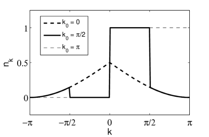
Figure 1: Initial $c$-fermion distributions for (a) no current ($k_{0}=0$), (b) non-zero current ($k_{0}=\pi/2$), and (c) maximum current ($k_{0}=\pi$). Note the sharp discontinuity for the case of non-zero current.

After the decay of transients $\left\langle c_{k}c_{-k}\right\rangle$, $\left\langle c^{\dagger}_{k}c^{\dagger}_{-k}\right\rangle$, we investigate the collective modes by employing the RPA analysis outlined in sub-section II.1. The RPA requires knowledge of the single-particle Green’s functions. The presence of a current does not affect the retarded Green’s function (Eq. (23)), but modifies the Keldysh Green’s function as follows

$$G^{K}_{f}(k;t,t^{\prime}) = -ie^{-i\epsilon_{k}(t-t^{\prime})}\left[\left|\sin\frac{k}{2}\right|(1-n_{k}-n_{-k})\right.$$ (36)

$$- \left.(n_{k}-n_{-k})\right],$$

where $n_{k}=\theta(k)\theta(k_{0}-k)\,$ is the occupation number of the $\eta$-fermions in the initial state.

III RPA for quench from ground state

In this section, we investigate the effect of interactions on the athermal steady state (sub-section II.1) obtained from quenching from the ground state of the transverse-field Ising model. The RPA particle-hole bubbles are

$$\Pi^{R}(q,\omega) = -\frac{1}{2}\int\frac{dk}{2\pi}\left[\frac{\cos\theta_{k}(1-2n_{k})}{(\omega+i\delta)+\epsilon_{k}-\epsilon_{k+q}}\right.$$ (37)

$$- \left.\frac{\cos\theta_{k+q}(1-2n_{k+q})}{(\omega+i\delta)+\epsilon_{k}-\epsilon_{k+q}}\right].$$

$$\Pi^{K}(q,\omega)=\frac{i}{2}(2\pi)\int\frac{dk}{2\pi}\delta(\omega+\epsilon_{k}-\epsilon_{k+q})$$

$$\times[\cos\theta_{k}\cos\theta_{k+q}(1-2n_{k})(1-2n_{k+q})-1].$$ (38)

For the case of interest, $\gamma=h/J=1$, we have $\cos\theta_{k}=\left|\sin\frac{k}{2}\right|$, and the distribution of the $\eta$ fermions $n_{k}=0$.

There are some basic symmetries of the polarization bubbles that are worth mentioning. Firstly $\Pi^{R,K}(q,\omega)=\Pi^{R,K}(-q,\omega)$, while ${\rm Re}[\Pi^{R}](q,-\omega)={\rm Re}[\Pi^{R}](q,\omega),\Pi^{K}(q,-\omega)=\Pi^{K}(q,\omega)$ and ${\rm Im}[\Pi^{R}(q,-\omega)]=-{\rm Im}[\Pi^{R}](q,\omega)$. Therefore in what follows we will assume $q>0,\omega>0$, and the results for the other regimes can be extrapolated from the above symmetries.

There are two regimes which we will study separately. One is $\omega>2J\sin\frac{q}{2}$ where ${\rm Im}[\Pi^{R}]=\Pi^{K}=0$, and the other is $\omega<2J\sin\frac{q}{2}$ where ${\rm Im}[\Pi^{R}]\neq 0,\Pi^{K}\neq 0$.

III.1 Evaluation for $\omega>2J\sin\frac{q}{2}$

In this regime, the integrand contains no poles, and the result is purely real: $\mbox{Re}\left[\Pi^{R}(q,\omega)\right]=\Pi^{R}(q,\omega)\,$ and $\mbox{Im}\left[\Pi^{R}(q,\omega)\right]=0$. One may safely take $\delta\rightarrow 0\,$ to find

$$\Pi^{R}(q,\omega)=\frac{-\cos\frac{q}{4}}{2\pi i\sqrt{\omega^{2}-(2J\sin\frac{q}{2})^{2}}}$$ (39)

$$\times \left\{z_{+}\ln\left[\frac{1+\frac{\sin\frac{q}{4}}{z_{+}}}{1-\frac{\sin\frac{q}{4}}{z_{+}}}\right]-z_{-}\ln\left[\frac{1+\frac{\sin\frac{q}{4}}{z_{-}}}{1-\frac{\sin\frac{q}{4}}{z_{-}}}\right]\right\}$$

$$- \frac{\sin\frac{q}{4}}{2\pi i\sqrt{\omega^{2}-(2J\sin\frac{q}{2})^{2}}}$$

$$\times \left\{z_{+}\ln\left[\frac{1+\frac{\cos\frac{q}{4}}{z_{+}}}{1-\frac{\cos\frac{q}{4}}{z_{+}}}\right]-z_{-}\ln\left[\frac{1+\frac{\cos\frac{q}{4}}{z_{-}}}{1-\frac{\cos\frac{q}{4}}{z_{-}}}\right]\right\},$$

with

$$z_{\pm}^{2} = \frac{1}{2}\pm\frac{1}{2}\sqrt{1-\left(\frac{\omega}{2J\sin\frac{q}{2}}\right)^{2}}\,\,\forall\omega<2J\sin\frac{q}{2}$$ (40)

$$= \frac{1}{2}\pm\frac{i}{2}\sqrt{\left(\frac{\omega}{2J\sin\frac{q}{2}}\right)^{2}-1}\,\,\forall\omega>2J\sin\frac{q}{2}$$

Note that our convention is to place the branch-cut of the logarithm on the negative real axis. In this same regime of $\omega>2J\sin\frac{q}{2}$ there are no roots to the argument of the delta function in the Keldysh component, and we have $\Pi^{K}(q,\omega)=0$. With $\Pi^{R}(q,\omega)\,$ purely real, this regime lies outside the particle-hole continuum. In sub-section III.3 we will demonstrate the existence of an undamped collective mode lying just above the particle-hole continuum for repulsive interactions only.

III.2 Evaluation for $\omega<2J\sin\frac{q}{2}$

For $\omega<2J\sin\frac{q}{2}\,$ the integrand generically contains poles. We extract the real and imaginary parts in the usual way by writing,

$$\int\frac{dk}{2\pi}\frac{f(k)}{\omega+i\delta+\epsilon_{k}-\epsilon_{k+q}}=\int\frac{dk}{2\pi}{\cal P}\left(\frac{f(k)}{\omega+\epsilon_{k}-\epsilon_{k+q}}\right)$$ (41)

$$-i\pi\int\frac{dk}{2\pi}f(k)\delta(\omega+\epsilon_{k}-\epsilon_{k+q})$$

$$\equiv \mbox{Re}\left[\Pi^{R}\right]+i\mbox{Im}\left[\Pi^{R}\right]$$ (42)

where ${\cal P}$ denotes taking the principal value of the integral. We obtain

$$\mbox{Re}\left[\Pi^{R}(q,\omega)\right]=\frac{-\cos\frac{q}{4}}{2\pi\sqrt{(2J\sin\frac{q}{2})^{2}-\omega^{2}}}$$ (43)

$$\times \left\{z_{+}\ln\left|\frac{1+\frac{\sin\frac{q}{4}}{z_{+}}}{1-\frac{\sin\frac{q}{4}}{z_{+}}}\right|-z_{-}\ln\left|\frac{1+\frac{\sin\frac{q}{4}}{z_{-}}}{1-\frac{\sin\frac{q}{4}}{z_{-}}}\right|\right\}$$

$$- \frac{\sin\frac{q}{4}}{2\pi\sqrt{(2J\sin\frac{q}{2})^{2}-\omega^{2}}}$$

$$\times \left\{z_{+}\ln\left|\frac{1+\frac{\cos\frac{q}{4}}{z_{+}}}{1-\frac{\cos\frac{q}{4}}{z_{+}}}\right|-z_{-}\ln\left|\frac{1+\frac{\cos\frac{q}{4}}{z_{-}}}{1-\frac{\cos\frac{q}{4}}{z_{-}}}\right|\right\},$$

with $z_{\pm}\,$ defined in Eq. (40). The results for the imaginary part, $\mbox{Im}\left[\Pi^{R}\right]=\frac{\Pi^{R}-\Pi^{A}}{2i}$, and the Keldysh component subdivide the particle-hole continuum into two sub-regions, $0<\omega<2J\sin^{2}\frac{q}{2}\,$ and $2J\sin^{2}\frac{q}{2}<\omega<2J\sin\frac{q}{2}$.

For $0<\omega<2J\sin^{2}\frac{q}{2}\,$ one finds

$$\mbox{Im}\left[\Pi^{R}(q,\omega)\right] = \frac{-1}{2\sqrt{(2J\sin\frac{q}{2})^{2}-\omega^{2}}}\left[\left(\cos\frac{q}{4}+\sin\frac{q}{4}\right)\right.$$ (44)

$$\times \left.\sin\left[\frac{1}{2}\sin^{-1}\frac{\omega}{2J\sin\frac{q}{2}}\right]\right]$$

$$\Pi^{K}(q,\omega) = \frac{i}{2\sqrt{(2J\sin\frac{q}{2})^{2}-\omega^{2}}}$$ (45)

$$\times \left[\cos\left(\sin^{-1}\left(\frac{\omega}{2J\sin\frac{q}{2}}\right)\right)-2\right].$$

whereas in the region $2J\sin^{2}\frac{q}{2}<\omega<2J\sin\frac{q}{2}$, the result is

$$\mbox{Im}\left[\Pi^{R}(q,\omega)\right] = \frac{-1}{2\sqrt{(2J\sin\frac{q}{2})^{2}-\omega^{2}}}$$ (46)

$$\times \left[\sin\frac{q}{4}\left(\sin\left[\frac{1}{2}\sin^{-1}\frac{\omega}{2J\sin\frac{q}{2}}\right]\right.\right.$$

$$+ \left.\left.\cos\left[\frac{1}{2}\sin^{-1}\frac{\omega}{2J\sin\frac{q}{2}}\right]\right)\right]$$

$$\Pi^{K}(q,\omega) = \frac{i}{2\sqrt{(2J\sin\frac{q}{2})^{2}-\omega^{2}}}\left[\cos\frac{q}{2}-2\right].$$ (47)

The particle-hole continuum, which is the region in $\omega,q$ space where ${\rm Im}\Pi^{R}\neq 0$ is indicated as the shaded region in Fig. 2 and compared with the equilibrium (no quench) result (inset). The two different shadings refer to the discontinuity in the functional forms of ${\rm Im}[\Pi]^{R},\Pi^{K}$ across $\omega=2J\sin^{2}\frac{q}{2}$. The consequences of these results are discussed below.

III.3 Undamped mode for $\omega>2J\sin\frac{q}{2}$ and $V_{0}>0$

The undamped mode is obtained from the solution of

$$1-V_{0}\Pi^{R}(q,\omega)=0$$ (48)

with $\Pi^{R}(q,\omega)$ given in Eq. (39). For sufficiently small $V_{0}$, we need to identify the points where $\Pi^{R}$ diverges. This occurs for $\omega=2J\sin(q/2)$. Thus in the limit of $\omega\rightarrow 2J\sin\frac{q}{2}$, we can write $z_{\pm}=\sqrt{\frac{1}{2}}\left(1\pm\frac{i\epsilon}{4J\sin\frac{q}{2}}\right)\,$ with $\epsilon=\sqrt{\omega^{2}-\left(2J\sin\frac{q}{2}\right)^{2}}$. The dominant contribution assuming that $q\rightarrow 0$ (so that $\cos\frac{q}{4}\approx 1$) is given by

$$\Pi^{R}(q,\omega) \simeq -\frac{\sin\frac{q}{4}}{2\pi i\sqrt{\omega^{2}-\left(2J\sin\frac{q}{2}\right)^{2}}}$$ (49)

$$\times \left\{z_{+}\ln\left[\frac{1+\sqrt{2}+i\frac{\epsilon\sqrt{2}}{4J\sin\frac{q}{2}}}{1-\sqrt{2}+i\frac{\epsilon\sqrt{2}}{4J\sin\frac{q}{2}}}\right]\right.$$

$$- \left.z_{-}\ln\left[\frac{1+\sqrt{2}-i\frac{\epsilon\sqrt{2}}{4J\sin\frac{q}{2}}}{1-\sqrt{2}-i\frac{\epsilon\sqrt{2}}{4J\sin\frac{q}{2}}}\right]\right\}.$$

Due to the branch-cut in the logarithm (chosen to be on the negative real axis), in the limit $\epsilon\rightarrow 0$, the above expression can be further simplified to give

$$\Pi^{R}(q,\omega) \simeq \frac{\sin\frac{q}{4}}{\sqrt{2}\sqrt{\omega^{2}-(2J\sin\frac{q}{2})^{2}}},$$ (50)

Thus from Eq. (48) we find a single undamped mode provided $V_{0}\,$ is positive with a dispersion

$$\omega_{q}\simeq\theta(V_{0})J|q|\sqrt{1+\frac{V_{0}^{2}}{32J^{2}}}.$$ (51)

This can be compared to the undamped mode in the equilibrium problem,dassarma2 ; dassarma

$$\omega_{q}^{\mbox{\scriptsize eq}}\simeq J|q|\sqrt{1+\frac{V_{0}}{\pi J}},$$ (52)

which exists for both attractive and repulsive interactions. Thus, for repulsive interactions, the obtained sound wave is qualitatively similar to the equilibrium case, but with a slightly modified velocity of propagation, whereas for attractive interactions, no undamped modes exist.

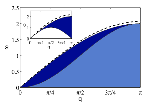
Figure 2: Undamped mode (dashed line) above the extended particle-hole continuum (shaded region). Inset: equilibrium continuum and undamped mode.

III.4 Enhanced particle-hole continuum and effective temperature

The highly broadened initial fermion distribution gives one way to define an effective temperature in this non-equilibrium state (cf. Eq. (19)). By analogy with the equilibrium properties of the particle-hole bubbles, one may define an effective temperature in terms of the collective degrees of freedom. Since the system is out of equilibrium, this temperature will in general depend on $\omega,q$ and also the chosen correlation function

$$\frac{\Pi^{R}(q,\omega)-\Pi^{A}(q,\omega)}{\Pi^{K}(q,\omega)}=\tanh\left(\frac{\omega}{2T^{\prime}_{\rm eff}(q,\omega)}\right).$$ (53)

For small frequencies, this ratio yields

$$\frac{\Pi^{R}-\Pi^{A}}{\Pi^{K}}\xrightarrow{\omega\rightarrow 0}\frac{\omega}{2J\sin\frac{q}{2}}\left(\sin\frac{q}{4}+\cos\frac{q}{4}\right),$$ (54)

so that for $\omega\rightarrow 0$, we obtain an effective-temperature

$$T^{\prime}_{\mbox{\scriptsize eff}}(q,\omega\rightarrow 0)=\frac{J\sin\frac{q}{2}}{\cos\frac{q}{4}+\sin\frac{q}{4}}.$$ (55)

We argue below that $T^{\prime}_{\rm eff}(q,\omega\rightarrow 0)$ is responsible for smearing out the particle-hole continuum in much the same way that temperature in an equilibrium system does. To see this recall that the particle-hole continuum represents the region in the $(q,\omega)$-plane where a collective mode of frequency $\omega\,$ and wave-vector $q\,$ is unstable to decay into single particle-hole excitations. The upper and lower continuum boundaries in equilibrium at zero temperature are given by Pearson62 ; todani

$$\omega_{L}(q)=J\sin q,$$ (56)

$$\omega_{U}(q)=2J\sin\frac{q}{2}.$$ (57)

A simple argument makes these boundaries plausible: consider the energy of a single particle-hole excitation which is created by removing a particle of momentum $k\,$ and creating a particle of momentum $k+q$,

$$\omega(k,q)=\epsilon_{k+q}-\epsilon_{k}=2J\sin\frac{q}{2}\sin\left(k+\frac{q}{2}\right).$$ (58)

This excitation energy depends not only on the momentum of the excitation, but also on the momentum of the original particle, $k$. For a half-filled band at zero temperature, the occupation of fermions is $\left\langle c_{k}^{\dagger}c_{k}\right\rangle_{\mbox{\scriptsize eq}}=\theta\left(\frac{\pi}{2}-|k|\right)$. The only momenta available for hole creation are those with $|k|<k_{F}=\frac{\pi}{2}$. Because the cosine dispersion has maximal slope at $k=\frac{\pi}{2}$, the maximum excitation energy occurs for a given $q\,$ with $k=\frac{\pi}{2}-\frac{q}{2}$. The smallest excitation energy for a given $q\,$ at zero temperature occurs at $k=\frac{\pi}{2}\,$ or $k=\frac{\pi}{2}-q$. Thus

$$\omega_{\mbox{\scriptsize max}}(q) = \omega\left(\frac{\pi}{2}-\frac{q}{2},q\right)=2J\sin\frac{q}{2},$$ (59)

$$\omega_{\mbox{\scriptsize min}}(q) = \omega\left(\frac{\pi}{2},q\right)=J\sin q.$$ (60)

which are just the upper and lower boundaries of the particle-hole continuum (inset Fig. 2). Now, consider lowering $k_{F}$. Excitations of smaller energy for a given $q\,$ are now possible, and in the limit $k_{F}\rightarrow 0$, we have $\omega_{\mbox{\scriptsize min}}\rightarrow 2J\sin^{2}\frac{q}{2}$. The result is the same if one considers the opposite limit of $k_{F}\rightarrow\pi\,$ at zero temperature.

In the present non-equilibrium situation, we find a particle-hole continuum ($\mbox{Im}\left[\Pi^{R}(q,\omega)\right]\neq 0$) that extends below this lower-bound all the way to $\omega=0$. A finite temperature is known to smear out this lower boundary,derzhko2 due to the smoothing out of the zero-temperature step function for the occupation probability. It is interesting to note that the expressions for $\mbox{Im}\left[\Pi^{R}(q,\omega)\right]\,$ and $\Pi^{K}(q,\omega)\,$ are actually continuous across the line $\omega=2J\sin^{2}\frac{q}{2}$, with discontinuities appearing in their derivatives. In Fig. 2 we plot the undamped collective mode dispersion with the particle-hole continuum represented by the shaded region. The two different shadings are separated by the line $\omega=2J\sin^{2}\frac{q}{2}$. The analogous plot for the equilibrium situation is shown in the inset.

IV RPA for current carrying state

We now apply RPA to study the current carrying non-equilibrium steady state described in section II.2. The Keldysh component of the fermion Green’s function is,

$$iG_{f}^{K}(k;t,t^{\prime}) = \left[\cos\theta_{k}(1-n_{k}-n_{-k})\right.$$ (61)

$$- \left.(n_{k}-n_{-k})\right]e^{-i\epsilon_{k}(t-t^{\prime})}.$$

while the retarded Green’s function is given in Eq. (23), and $n_{k}=\theta(k)\theta(k_{0}-k)$. Eq. (61) implies that the distribution function for the Jordan-Wigner fermions in the current carrying post-quench state is not only broad as for the zero current case, but is also asymmetric in $k$, with sharp discontinuities superimposed on it (see Fig. 1). Thus we will find that as for the zero-current case, the particle-hole continuum here too is broadened (extending everywhere below the line $\omega_{\rm max}=2J\sin\frac{q}{2}$), while the sharp structure in the distribution gives rise to some discontinuities in the expression for ${\rm Im}[\Pi^{R}]$, and the appearance of additional damped modes.

The particle-hole bubbles are now given by

$$\Pi^{R}(q,\omega) = -\frac{1}{2}\int\frac{dk}{2\pi}\left[\frac{\cos\theta_{k}(1-n_{k}-n_{-k})}{\omega+i\delta-2J\sin\frac{q}{2}\sin\left(k+\frac{q}{2}\right)}\right.$$ (62)

$$- \frac{(n_{k}-n_{-k})}{\omega+i\delta-2J\sin\frac{q}{2}\sin\left(k+\frac{q}{2}\right)}$$

$$- \frac{\cos\theta_{k+q}(1-n_{k+q}-n_{-k-q})}{\omega+i\delta-2J\sin\frac{q}{2}\sin\left(k+\frac{q}{2}\right)}$$

$$+ \left.\frac{(n_{k+q}-n_{-k-q})}{\omega+i\delta-2J\sin\frac{q}{2}\sin\left(k+\frac{q}{2}\right)}\right]$$

$$\Pi^{K}(q,\omega)=\frac{i}{2}(2\pi)\int\frac{dk}{2\pi}\delta(\omega+\epsilon_{k}-\epsilon_{k+q})$$

$$\times\left\{\left[\cos\theta_{k}(1-n_{k}-n_{-k})-(n_{k}-n_{-k})\right]\right.$$

$$\times\left[\cos\theta_{k+q}(1-n_{k+q}-n_{-k-q})-(n_{k+q}-n_{-k-q})\right]$$

$$\left.-1\right\}.$$ (63)

As before two regions appear, one where $\omega>2J\sin\frac{q}{2}$ for which ${\rm Im}[\Pi^{R}]=\Pi^{K}=0$, and the second being $\omega<2J\sin\frac{q}{2}$ where a particle-hole continuum is found to exist. We discuss these two regions separately.

IV.1 Evaluation for $\omega>2J\sin\frac{q}{2}$

In this regime, as before, the result is entirely real and we let $\delta\rightarrow 0$. We find it convenient to write $\Pi^{R}=\Pi^{(1)}+\Pi^{(2)}$, where $\Pi^{(1)}\,$ depends on the Bogoliubov angle, $\cos\theta_{k}=\left|\sin\frac{k}{2}\right|$, while $\Pi^{(2)}$ contains the rest. As before it is convenient to summarize the symmetries of the polarization bubbles. We find $\Pi^{(1)}(-q,\omega)=\Pi^{(1)}(q,\omega)$, however due to current flow, $\Pi^{(2)}(-q,\omega)=-\Pi^{(2)}(q,\omega)$. Similarly, ${\rm Re}[\Pi^{(1)}](q,-\omega)={\rm Re}[\Pi^{(1)}](q,\omega)$, while ${\rm Re}[\Pi^{(2)}](q,-\omega)=-{\rm Re}[\Pi^{(2)}](q,\omega)$. In the discussion that follows, we take $q>0,\omega>0$.

We find,

$$\Pi^{(1)}(q,\omega)=-\frac{\cos\frac{q}{4}}{4\pi i\sqrt{\omega^{2}-(2J\sin\frac{q}{2})^{2}}}$$ (64)

$$\times \left\{\mathcal{F}\left(\sin\left[\frac{k_{0}}{2}+\frac{q}{4}\right]\right)+\mathcal{F}\left(\sin\left[-\frac{k_{0}}{2}+\frac{q}{4}\right]\right)\right\}$$

$$- \frac{\sin\frac{q}{4}}{4\pi i\sqrt{\omega^{2}-(2J\sin\frac{q}{2})^{2}}}$$

$$\times \left\{\mathcal{F}\left(\cos\left[\frac{k_{0}}{2}+\frac{q}{4}\right]\right)+\mathcal{F}\left(\cos\left[-\frac{k_{0}}{2}+\frac{q}{4}\right]\right)\right\},$$

where

$$\mathcal{F}(z)=z_{+}\ln\left[\frac{\left(1+\frac{z}{z_{+}}\right)}{\left(1-\frac{z}{z_{+}}\right)}\right]-z_{-}\ln\left[\frac{\left(1+\frac{z}{z_{-}}\right)}{\left(1-\frac{z}{z_{-}}\right)}\right].$$ (65)

In the limit $k_{0}\rightarrow 0$, we recover the results of section III. The remaining terms can be collected as

$$\Pi^{(2)}=\frac{1}{4\pi}\left\{\int_{k_{0}-q/2}^{k_{0}+q/2}-\int_{-q/2}^{q/2}\right\}$$

$$\times dk\left\{\frac{1}{\omega-2J\sin\frac{q}{2}\sin k}+\frac{1}{\omega+2J\sin\frac{q}{2}\sin k}\right\}$$

$$= -\frac{1}{4\pi i\sqrt{\omega^{2}-(2J\sin\frac{q}{2})^{2}}}$$

$$\times \left\{\ln\left[\frac{1+\frac{\omega\tan\left(\frac{k_{0}}{2}+\frac{q}{4}\right)}{4J\sin\frac{q}{2}z_{+}^{2}}}{1-\frac{\omega\tan\left(\frac{k_{0}}{2}+\frac{q}{4}\right)}{4J\sin\frac{q}{2}z_{+}^{2}}}\right]-\ln\left[\frac{1+\frac{\omega\tan\left(\frac{k_{0}}{2}-\frac{q}{4}\right)}{4J\sin\frac{q}{2}z_{+}^{2}}}{1-\frac{\omega\tan\left(\frac{k_{0}}{2}-\frac{q}{4}\right)}{4J\sin\frac{q}{2}z_{+}^{2}}}\right]\right.$$

$$- \ln\left[\frac{1+\frac{\omega\tan\left(\frac{k_{0}}{2}+\frac{q}{4}\right)}{4J\sin\frac{q}{2}z_{-}^{2}}}{1-\frac{\omega\tan\left(\frac{k_{0}}{2}+\frac{q}{4}\right)}{4J\sin\frac{q}{2}z_{-}^{2}}}\right]+\ln\left[\frac{1+\frac{\omega\tan\left(\frac{k_{0}}{2}-\frac{q}{4}\right)}{4J\sin\frac{q}{2}z_{-}^{2}}}{1-\frac{\omega\tan\left(\frac{k_{0}}{2}-\frac{q}{4}\right)}{4J\sin\frac{q}{2}z_{-}^{2}}}\right]$$

$$- \left.2\ln\left[\frac{1+\frac{\omega\tan\left(\frac{q}{4}\right)}{4J\sin\frac{q}{2}z_{+}^{2}}}{1-\frac{\omega\tan\left(\frac{q}{4}\right)}{4J\sin\frac{q}{2}z_{+}^{2}}}\right]+2\ln\left[\frac{1+\frac{\omega\tan\left(\frac{q}{4}\right)}{4J\sin\frac{q}{2}z_{-}^{2}}}{1-\frac{\omega\tan\left(\frac{q}{4}\right)}{4J\sin\frac{q}{2}z_{-}^{2}}}\right]\right\},$$ (67)

The consequence of the above expressions for $\Pi^{(1,2)}$ will be discussed in section IV.3.

IV.2 Evaluation for $\omega<2J\sin\frac{q}{2}$

In this regime, the real part of $\Pi^{R}(q,\omega)\,$ is given by the principal value of the integral in Eq. (62). Writing $\mbox{Re}\left[\Pi^{R}(q,\omega)\right]={\rm Re}[{\Pi}^{(1)}]+{\rm Re}[{\Pi}^{(2)}]$, where

$${\rm Re}[{\Pi}^{(1)}](q,\omega)=-\frac{\cos\frac{q}{4}}{4\pi\sqrt{(2J\sin\frac{q}{2})^{2}-\omega^{2}}}$$ (68)

$$\times \left\{\tilde{\mathcal{F}}\left(\sin\left[\frac{k_{0}}{2}+\frac{q}{4}\right]\right)+\tilde{\mathcal{F}}\left(\sin\left[-\frac{k_{0}}{2}+\frac{q}{4}\right]\right)\right\}$$

$$- \frac{\sin\frac{q}{4}}{4\pi\sqrt{(2J\sin\frac{q}{2})^{2}-\omega^{2}}}$$

$$\times \left\{\tilde{\mathcal{F}}\left(\cos\left[\frac{k_{0}}{2}+\frac{q}{4}\right]\right)+\tilde{\mathcal{F}}\left(\cos\left[-\frac{k_{0}}{2}+\frac{q}{4}\right]\right)\right\},$$

where

$$\tilde{\mathcal{F}}(z)=z_{+}\ln\left|\frac{\left(1+\frac{z}{z_{+}}\right)}{\left(1-\frac{z}{z_{+}}\right)}\right|-z_{-}\ln\left|\frac{\left(1+\frac{z}{z_{-}}\right)}{\left(1-\frac{z}{z_{-}}\right)}\right|,$$ (69)

and

$${\rm Re}[\Pi^{(2)}](q,\omega)=-\frac{1}{4\pi\sqrt{(2J\sin\frac{q}{2})^{2}-\omega^{2}}}$$

$$\times\left\{\ln\left|\frac{1+\frac{\omega\tan\left(\frac{k_{0}}{2}+\frac{q}{4}\right)}{4J\sin\frac{q}{2}z_{+}^{2}}}{1-\frac{\omega\tan\left(\frac{k_{0}}{2}+\frac{q}{4}\right)}{4J\sin\frac{q}{2}z_{+}^{2}}}\right|-\ln\left|\frac{1+\frac{\omega\tan\left(\frac{k_{0}}{2}-\frac{q}{4}\right)}{4J\sin\frac{q}{2}z_{+}^{2}}}{1-\frac{\omega\tan\left(\frac{k_{0}}{2}-\frac{q}{4}\right)}{4J\sin\frac{q}{2}z_{+}^{2}}}\right|\right.$$

$$-\ln\left|\frac{1+\frac{\omega\tan\left(\frac{k_{0}}{2}+\frac{q}{4}\right)}{4J\sin\frac{q}{2}z_{-}^{2}}}{1-\frac{\omega\tan\left(\frac{k_{0}}{2}+\frac{q}{4}\right)}{4J\sin\frac{q}{2}z_{-}^{2}}}\right|+\ln\left|\frac{1+\frac{\omega\tan\left(\frac{k_{0}}{2}-\frac{q}{4}\right)}{4J\sin\frac{q}{2}z_{-}^{2}}}{1-\frac{\omega\tan\left(\frac{k_{0}}{2}-\frac{q}{4}\right)}{4J\sin\frac{q}{2}z_{-}^{2}}}\right|$$

$$-\left.2\ln\left|\frac{1+\frac{\omega\tan\left(\frac{q}{4}\right)}{4J\sin\frac{q}{2}z_{+}^{2}}}{1-\frac{\omega\tan\left(\frac{q}{4}\right)}{4J\sin\frac{q}{2}z_{+}^{2}}}\right|+2\ln\left|\frac{1+\frac{\omega\tan\left(\frac{q}{4}\right)}{4J\sin\frac{q}{2}z_{-}^{2}}}{1-\frac{\omega\tan\left(\frac{q}{4}\right)}{4J\sin\frac{q}{2}z_{-}^{2}}}\right|\right\},$$ (70)

We do not give expressions for $\mbox{Im}\left[\Pi^{R}\right],\Pi^{K}$ as the boundaries of the particle-hole continuum are the same as in Fig. 2, though there are additional discontinuities within the continuum besides the one along $\omega=2J\sin^{2}\frac{q}{2}$. Instead in the subsequent sections, by studying the divergences in ${\rm Re}[\Pi^{R}]$ we will identify a single undamped mode for repulsive interactions and $k_{0}<\pi/2$, and several damped modes for both repulsive and attractive interactions.

IV.3 Undamped mode for $\omega>2J\sin\frac{q}{2}$ and $V_{0}>0$

In this section we demonstrate that an undamped collective mode survives provided the current is not too large. As before, define $\epsilon=\sqrt{\omega^{2}-\left(2J\sin\frac{q}{2}\right)^{2}}$. In the limit $q\rightarrow 0\,$ and for small $k_{0}$, the most divergent terms in $\Pi^{R}(q,\omega)\,$ are

$$\Pi^{R}(q,\omega) \simeq -\frac{\sin\frac{q}{4}}{4\pi\sqrt{\left(2J\sin\frac{q}{2}\right)^{2}-\omega^{2}}}\left\{\mathcal{F}\left[\cos\left(\frac{k_{0}}{2}\right)\right]\right.$$

$$+ \left.\mathcal{F}\left[\cos\left(-\frac{k_{0}}{2}\right)\right]\right\}$$

$$\simeq \frac{\sin\frac{q}{4}}{2\pi i\sqrt{2}\sqrt{\omega^{2}-(2J\sin\frac{q}{2})^{2}}}$$

$$\times \left\{\ln\left[1-\sqrt{2}\cos\frac{k_{0}}{2}+i\frac{\epsilon\sqrt{2}\cos\frac{k_{0}}{2}}{2J\sin\frac{q}{2}}\right]\right.$$

$$- \left.\ln\left[1-\sqrt{2}\cos\frac{k_{0}}{2}-i\frac{\epsilon\sqrt{2}\cos\frac{k_{0}}{2}}{2J\sin\frac{q}{2}}\right]\right\}$$ (72)

The above expression shows that provided $k_{0}<\frac{\pi}{2}$, which corresponds to the logarithms having a branch-cut, we obtain

$$\Pi^{R}(q,\omega) = \frac{\sin\frac{q}{4}}{\sqrt{2}\sqrt{\omega^{2}-(2J\sin\frac{q}{2})^{2}}},$$ (73)

Thus by setting $1-V_{0}\Pi^{R}=0$, we recover the same dispersion as in the absence of current

$$\omega_{q}\simeq J|q|\sqrt{1+\frac{V_{0}^{2}}{32J^{2}}}\theta(V_{0})\theta(\pi/2-k_{0})$$ (74)

Thus, the undamped mode is unchanged for a current which is below the threshold value of $k_{0}<\pi/2$. On the other hand, for currents larger than this value ($k_{0}>\pi/2$) and for $q\ll k_{0}$, no undamped modes exist.

IV.4 Damped modes for $\omega<2J\sin\frac{q}{2}$

In this regime, all modes are damped. We identify these damped modes by looking for solutions to $1-V_{0}{\rm Re}[\Pi^{R}](q,\omega_{q})=0$. For $V_{0}\rightarrow 0$, all we need to do is identify where $\mbox{Re}\left[\Pi^{R}\right]\rightarrow\pm\infty$. Then positive divergences correspond to damped modes with repulsive interactions, while negative divergences correspond to damped modes with attractive interactions.

Upon examining Eqns. (68) and  (70), we find logarithmic divergences in $\mbox{Re}\left[\Pi^{R}(q,\omega)\right]\,$ along the characteristic lines (for $\omega,q>0$)

$$\omega_{1}(q) = 2J\sin^{2}\frac{q}{2},$$ (75)

$$\omega_{2}(q) = 2J\sin\frac{q}{2}\sin\left(k_{0}+\frac{q}{2}\right),$$ (76)

$$\omega_{3}^{\pm}(q) = \pm 2J\sin\frac{q}{2}\sin\left(\frac{q}{2}-k_{0}\right),$$ (77)

Note that $\omega_{2,3}$ coincide with the characteristic lines in the equilibrium problem with an arbitrary Fermi momentum $k_{0}$.derzhko2 In the equilibrium problem, these lines represent boundaries across which $\mbox{Im}\left[\Pi^{R}\right]\,$ undergoes a jump discontinuity. This is also the case here, though we will focus our attention on the behavior of the real part.

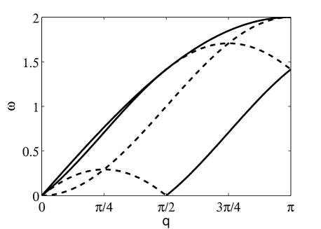
Figure 3: Characteristic lines along which $\mbox{Re}\left[\Pi^{R}(q,\omega)\right]\,$ diverges, giving rise to damped modes for repulsive (solid lines) and attractive (dashed lines) interactions for $k_{0}=\frac{\pi}{4}$. Only the top line $\omega=2J\sin\frac{q}{2}\,$ corresponds to an undamped mode existing above the particle-hole continuum.

One finds $\mbox{Re}\left[\Pi^{R}\right]\rightarrow+\infty\,$ along the line $\omega_{3}^{+}(q)\,$ for $2k_{0}<q<\pi\,$ and along the line $\omega_{2}(q)\,$ for $q<\pi-2k_{0}$. These correspond to damped collective modes for repulsive interactions. Furthermore, $\mbox{Re}\left[\Pi^{R}\right]\rightarrow-\infty\,$ along the line $\omega_{1}(q)\,$ for all $q\in(0,\pi)$, along $\omega_{3}^{-}(q)\,$ for $q<2k_{0}$, and along $\omega_{2}(q)\,$ for $q>\pi-2k_{0}$. These negative divergences represent collective modes created by attractive interactions. We plot these characteristic lines in Fig. 3 and indicate whether the mode exists for attractive or repulsive interactions.

Such damped modes are usually considered physically uninterestingdassarma compared to any undamped excitations in the system, as the damping makes these modes experimentally unobservable. The divergences in $\Pi^{R}(q,\omega)\,$ that give rise to these damped modes are of a different nature than those giving rise to the undamped mode. To see this consider the case of $\omega\simeq\omega_{1}=2J\sin\frac{q}{2}\left(\sin\frac{q}{2}\pm\epsilon\right)\,$ for small $\epsilon$. The dominant contribution is given by

$$\mbox{Re}\left[\Pi^{R}(q,\omega)\right]\simeq\frac{-1}{8\pi J\sin\frac{q}{2}\left|\cos\frac{q}{2}\right|}\left[2\log\frac{A_{q}}{\epsilon}\right].$$ (78)

where $A_{q}$ is a $q$-dependent factor.

Solving $1=V_{0}\mbox{Re}\Pi^{R}\left[(q,\omega_{q})\right]\,$ to leading order in $\epsilon$, one finds

$$\mbox{Re}\left[\omega_{q}\right]\simeq 2J\sin\frac{q}{2}\left(\sin\frac{q}{2}\pm A_{q}e^{-(2\pi J\sin q)/|V_{0}|}\right),$$ (79)

where $q>0\,$ is assumed. In general, for any of the characteristic lines described above, the ansatz $\omega=\omega_{c}\pm 2J\epsilon\sin\frac{q}{2}\,$ leads to a divergence of the form $\Pi^{R}(q,\omega)\sim\pm\log\frac{1}{\epsilon}$. Each logarithmic divergence corresponds to two damped modes lying exponentially close to each characteristic line.

One may study the modes near $\omega\approx\omega_{2}(q)\,$ in a way similar to our analysis for the modes near $\omega_{1}$. For $\omega\approx\omega_{2}(q)\pm 2J\epsilon\sin\frac{q}{2}$, one finds

$$\mbox{Re}\left[\Pi^{R}(q,\omega)\right]\simeq\frac{1+\sin\frac{k_{0}}{2}}{8\pi J\sin\frac{q}{2}\left|\cos\left(k_{0}+\frac{q}{2}\right)\right|}\log\frac{A^{\prime}_{q}}{\epsilon},$$ (80)

which gives rise to damped modes for repulsive interactions ($V_{0}>0$) when $q<\pi-2k_{0}$ with

$$\mbox{Re}\left[\omega_{q}\right]\simeq 2J\sin\frac{q}{2}\left(\sin\left(\frac{q}{2}+k_{0}\right)\right.$$ (81)

$$\pm \left.A_{q}^{\prime}\exp\left[-\frac{8\pi J\sin\frac{q}{2}\left|\cos\left(k_{0}+\frac{q}{2}\right)\right|}{V_{0}\left(1+\sin\frac{k_{0}}{2}\right)}\right]\right).$$

The results for the other characteristic line $\omega_{3}^{+}$ is similar and we do not discuss it further.

V Summary and Conclusions

In this paper, we have applied the RPA to study the effect of weak Ising interactions in a non-equilibrium steady state of the $XXZ\,$ spin chain. This non-equilibrium state was created in two different ways. One is by quenching from the ground state of the transverse-field Ising model at critical magnetic field to the $XX$-model. The second was to modify the Hamiltonian before the quench by adding Dzyaloshinskii-Moriya interactions. This had the effect of creating a current carrying state.

The RPA for both the steady-states shows the existence of a single, undamped, collective mode for repulsive interactions which is qualitatively similar to the sound mode in equilibrium, but with quantitative changes to the mode velocity (c.f. Eq. (51)). However if the current is larger than a threshold value, this undamped mode ceases to exist in the long-wavelength limit (c.f. Eq. (74)). The primary effect of the quench is to give rise to a highly broadened distribution function (c.f. Fig. 1, Eq. (35)) which results in an enhanced particle-hole continuum. The boundaries of the particle-hole continuum are shown in Fig. 2. Thus for attractive interactions either no modes are found for the first steady-state, or some damped collective modes are found for the steady-state with current.

These results, and in particular the generation of a finite friction due to an out of equilibrium situation, are rather generic and do not depend on the details of the non-equilibrium steady-state. Further, the upper boundary of the particle-hole continuum occurs at $\omega_{\rm max}=2J\sin\frac{q}{2}$ and is related to the fact that the system is on a lattice, and therefore the excitations have a maximum velocity. If instead a quadratic dispersion for the fermions is adopted, then there is no upper-limit to the velocity of excitations. This together with the fact that immediately after a quench, the Fermi-distribution is very broad with no well defined $k_{F}$ will further enhance the upper boundary of the particle-hole continuum, damping even the mode with repulsive interactions.

An important future direction for research is to explore how these results change when an explicit time-dependence on $J^{z}$ is introduced. In particular it is important to understand how slowly $J^{z}$ has to be turned on in order to recover the results of this paper.

Acknowledgments: This work was supported by NSF DMR (Grant No. 1004589) (JL and AM) and by the Swiss SNF under MaNEP and Division II (TG).

References

• (1) T. Kinoshita, T. Wenger, and D. S. Weiss, Nature (London) 440, 900 (2006).
• (2) A. Polkovnikov, K. Sengupta, A. Silva, and M. Vengalattore, arXiv:1007.5331.
• (3) J. S. Caux and J. Mossel, J. Stat. Mech. P02023 (2011).
• (4) J. Mossel and J. S. Caux, New J. Phys. 12, 055028 (2010).
• (5) J. Lancaster and A. Mitra, Phys. Rev. E 81, 061134 (2010).
• (6) M. A. Cazalilla, Phys. Rev. Lett. 97, 156403 (2006).
• (7) A. Iucci and M. A. Cazalilla, Phys. Rev. A 80, 063619 (2009).
• (8) A. Iucci and M. A. Cazalilla, New J. Phys. 12, 055019 (2010).
• (9) T. Antal, Z. Rácz, A. Rákos, G. M. Schütz, Phys. Rev. E 59, 4912 (1999).
• (10) D. M. Kennes and V. Meden, Phys. Rev. B 82, 085109 (2010).
• (11) D. Gobert, C. Kollath, U. Schollwöck, and G Schütz, Phys. Rev. E 71, 036102 (2005).
• (12) S. Trotzky, Y. Chen, A. Flesch, I. P. McCulloch, U. Schollwöck, J. Eisert, and I. Bloch, arXiv:1101.2659.
• (13) M. Rigol, Phys. Rev. Lett. 103, 100403 (2009); Phys. Rev. A 80, 053607 (2009).
• (14) L. Santos and M. Rigol, Phys. Rev. E 81, 036206 (2010).
• (15) M. Rigol, V. Dunjko, V. Yurovsky, and M. Olshanii, Phys. Rev. Lett. 98, 050405 (2007).
• (16) P. Calabrese and J. Cardy, Phys. Rev. Lett. 96, 136801 (2006).
• (17) T. Barthel and U. Schollwöck, Phys. Rev. Lett. 100, 100601 (2008).
• (18) D. M. Gangardt and M. Pustilnik, Phys. Rev. A 77, 041604 (2008).
• (19) D. Rossini, S. Suzuki, G. Mussardo, G. E. Santoro, and A. Silva, Phys. Rev. B 82, 144302 (2010).
• (20) T. Caneva, E. Canovi, D. Rossini G. E. Santoro, and A. Silva, arXiv:1105.3176.
• (21) A. Mitra and T. Giamarchi, arXiv:1105.0124.
• (22) I. E. Dzyaloshinskii and A. I. Larkin, Zh. Eksp. Tero. Fiz. 38, 202 (1974).
• (23) H. U. Everts and H. Schulz, Solid State Comm. 15 1413 (1974).
• (24) C. Dover, Ann. Phys. 50, 500 (1968).
• (25) T. Giamarchi, Quantum Physics in One Dimension (Oxford University Press, Oxford, 2004).
• (26) Q. P. Li, S. Das Sarma, and R. Joynt, Phys. Rev. B 45, 13713 (1992).
• (27) S. Das Sarma and E. H. Hwang, Phys. Rev. B 54, 1936 (1996).
• (28) E. Lieb, T. Schultz, and D. Mattis, Ann. Phys. (N.Y.) 16, 407 (1961).
• (29) E. Barouch and B. McCoy, Phys. Rev. A 3, 2137-2140 (1971).
• (30) J. H. Taylor and G. Müller, Physica 130A, 1 (1985).
• (31) R. W. Cherng and L. S. Levitov, Phys. Rev. A 73, 043614 (2006).
• (32) Tomaz̆ Prosen and Iztok Piz̆orn, Phys. Rev. Lett. 101, 105701 (2008).
• (33) S. Sachdev Quantum Phase Transitions (Cambridge University Press, Cambridge, England, 1999).
• (34) P. Calabrese, F. H. L. Essler and M. Fagotti, Phys. Rev. Lett. 106, 227203 (2011).
• (35) A. Kamenev and A. Levchenko, Adv. Phys. 58, 197 (2009).
• (36) I. E. Dzyaloshinskii, J. Phys. Chem. Solids 4, 241 (1958); T. Moriya, Phys. Rev. 120, 91 (1960).
• (37) O. Derzhko, T. Verkholyak, T. Krokhmalskii and H. Büttner, Phys. Rev. B 73, 214407 (2006).
• (38) Th. J. Siskens, H. W. Capel, K. J. F. Gaemers, Physica 79A, 259 (1975).
• (39) J. H. H. Perk and H. W. Capel, Phys. Lett. A 58, 115 (1976).
• (40) T. Antal, Z. Rácz, A. Rákos, G. M. Schütz, Phys. Rev. E 57, 5184 (1998).
• (41) A. Das, S. Garnerone, S. Haas, arXiv:1104.5467.
• (42) J. des Cloizeaux and J. J. Pearson, Phys. Rev. 128, 2131 (1962)
• (43) T. Todani and K. Kawasaki, Prog. Theor. Phys. 50, 1216 (1973).
• (44) T. Verkholyak, O. Derzhko, T. Krokhmalskii, and J. Stolze, Phys. Rev. B 76, 144418 (2007).