A New Outer-Bound via Interference Localization and the Degrees of Freedom Regions of MIMO Interference Networks with no CSIT

Abstract

The two-user multi-input, multi-output (MIMO) interference and cognitive radio channels are studied under the assumption of no channel state information at the transmitter (CSIT) from the degrees of freedom (DoF) region perspective. With $M_{i}$ and $N_{i}$ denoting the number of antennas at transmitter $i$ and receiver $i$ respectively, the DoF regions of the MIMO interference channel were recently characterized by Huang et al., Zhu and Guo, and by the authors of this paper for all values of numbers of antennas except when $\min(M_{1},N_{1})>N_{2}>M_{2}$ (or $\min(M_{2},N_{2})>N_{1}>M_{1}$). This latter case was solved more recently by Zhu and Guo who provided a tight outer-bound. Here, a simpler and more widely applicable proof of that outer-bound is given based on the idea of interference localization. Using it, the DoF region is also established for the class of MIMO cognitive radio channels when $\min(M_{1}+M_{2},N_{1})>N_{2}>M_{2}$ (with the second transmitter cognitive) – the only class for which the inner and outer bounds previously obtained by the authors were not tight – thereby completing the DoF region characterization of the general 2-user MIMO cognitive radio channel as well.

I Introduction

Consider a multiple-input multiple-output (MIMO) interference channel (IC) consisting of two transmitters, T1 and T2, equipped with $M_{1}$ and $M_{2}$ antennas, respectively, and their paired or intended receivers R1 and R2 having $N_{1}$ and $N_{2}$ antennas, respectively. Each transmitter must communicate its message to its paired receiver over a shared additive Gaussian noise channel so that its transmission produces interference at the unpaired receiver. Denote such a channel as the $(M_{1},M_{2},N_{1},N_{2})$ MIMO IC. The input-output relationship in this MIMO IC is given as

$$\mbox{R1: }\hskip 1.0ptY(t)=H^{11}(t)X^{1}(t)+H^{12}(t)X^{2}(t)+W(t),$$ (1)

$$\mbox{R2: }Z(t)=H^{21}(t)X^{1}(t)+H^{22}(t)X^{2}(t)+W^{\prime}(t),$$ (2)

where at the $t^{th}$ channel use, $Y(t)\in\mathbb{C}^{N_{1}\times 1}$ and $Z(t)\in\mathbb{C}^{N_{2}\times 1}$ are the signals received by R1 and R2, respectively; $X^{1}(t)\in\mathbb{C}^{M_{1}\times 1}$ and $X^{2}(t)\in\mathbb{C}^{M_{2}\times 1}$ are the signals transmitted by T1 and T2, respectively; $W(t)$ and $W^{\prime}(t)$ are the additive white Gaussian noises; $H^{ij}(t)\in\mathbb{C}^{N_{i}\times M_{j}}$ represents the channel matrix between Tj and Ri, $i,j\in\{1,2\}$; there is a power constraint of $P$ at both transmitters, i.e.,

$$\lim_{b\to\infty}\frac{1}{b}\sum_{t=1}^{b}\mathbb{E}||X_{i}(t)||^{2}\leq P,~{}i=1,2.$$

Recently, [1, 2, 3] studied the DoF region of the MIMO IC with CSIR (i.e., with receivers having perfect channel knowledge) but with no CSIT. They provided inner and outer-bounds to the DoF region which coincide for a large class of MIMO ICs. In particular, these bounds yield the exact characterization of the no-CSIT DoF region except if either of the two inequalities, namely, $\min(M_{1},N_{1})>N_{2}>M_{2}$ or its symmetric counterpart, namely $\min(M_{2},N_{2})>N_{1}>M_{1}$, holds. For this latter class, [4] more recently obtained a tight outer-bound and proved that the inner-bound proposed earlier in [1, 2, 3] is indeed equal to the DoF region. The DoF region of the MIMO IC was determined earlier under the idealized CSIT (and CSIR) assumption in [5, 6].

Henceforth, MIMO ICs of interest in this work for which $\min(M_{1},N_{1})>N_{2}>M_{2}$ will be referred to as having asymmetrically constrained transmitters. In the following, we describe briefly why the outer-bounds of [1, 2, 3] are not tight for such MIMO ICs. Suppose $d_{2}$ DoF are to be achieved for the second (T2-R2) pair. Then, Fano’s inequality [7] can be used to show that the total interference at R2 can not have a multiplexing gain higher than $N_{2}-d_{2}$. Since the interference at R2 is caused by the transmission of T1, this condition puts constraints on $X^{1}(t)$, and hence on $d_{1}$ (the DoF of first pair T1-R1). Indeed, an outer-bound derived based on this idea suffices to characterize the no-CSIT DoF regions of all MIMO ICs except those with asymmetrically constrained transmitters. In this latter case, since $M_{2}<N_{2}$, the transmit signal of T2, namely, $X^{2}(t)$ can not span the entire $N_{2}$-dimensional receive-signal space of R2. Thus, if $d_{2}$ DoF are to be achieved for the second pair, the interference at R2 should satisfy not just the constraint that its multiplexing gain can not exceed $N_{2}-d_{2}$, but also that there exists an $M_{2}$-dimensional subspace at R2 which carries interference whose multiplexing gain is not more than $M_{2}-d_{2}$; because if any $M_{2}$-dimensional subspace at R2 contains interference with multiplexing gain (strictly) more than $M_{2}-d_{2}$, then R2 can not achieve $d_{2}$ DoF by decoding $X^{2}(t)$ since $X^{2}(t)$ lies within just an $M_{2}$-dimensional subspace. Accounting for this latter constraint becomes crucial for an IC with asymmetrically constrained transmitters because the condition $M_{1},N_{1}>N_{2}$ ensures that T1 can transmit a signal that violates this latter constraint (while R1 is still able to decode its desired signal). Thus, when $M_{2}<N_{2}<\min(M_{1},N_{1})$, one must consider a stricter constraint which, in essence, dictates that the interference at R2 can not be distributed arbitrarily in the receive signal-space of R2. This notion, which at $d_{2}=M_{2}$ asserts that the interference is localized within some $(N_{2}-M_{2})$-dimensional subspace, is referred to henceforth as interference localization. Indeed, it is because the outer-bounds derived in [1, 2, 3] do not use this stronger constraint that they fail to characterize the DoF region of the ICs with asymmetrically constrained transmitters. Section III-A provides a more detailed heuristic explanation. On the other hand, in [4], the authors overcome this problem by first showing that it is DoF-region optimal for T2 to transmit $X^{2}(t)$ which is Gaussian with a covariance matrix that is proportional to the identity matrix. Consequently, with such an $X^{2}(t)$, they prove that the $M_{2}$-dimensional subspace spanned by $X^{2}(t)$ at R2 can not carry interference with a non-zero multiplexing gain. In a way, this latter point can be seen to implicitly capture the idea of interference localization described above.

In this paper, we provide a simpler and more generic proof of the result of [4]. Unlike in [4], our proof does not require specialized techniques such as showing that the DoF-region optimality is retained by restricting $X_{2}$ to be Gaussian. Instead, the proof here makes use of basic information-theoretic identities such as the chain rules for differential entropy and mutual information, conditioning reduces entropy, etc. Consequently, the techniques developed here have the potential to be applicable for a wider class of networks.

As a case in point, we also study here the MIMO cognitive radio channel (CRC) [8], which is defined as the MIMO IC with T2 cognitive (i.e., T2 knows the message of T1 as well). For the MIMO CRC, we determine the no-CSIT DoF region for the only class of MIMO CRCs for which the inner and outer-bounds established earlier by the authors in [3] were not tight, namely, that defined by the inequality $\min(M_{1}+M_{2},N_{1})>N_{2}>M_{2}$. Our result here therefore completes the DoF region characterization of the MIMO CRC. In contrast, the applicability of the approach of [4] is unclear, because it is not clear if the optimality of Gaussian $X_{2}$ can be proved in this problem, which is a critical step in the proof of [4]. The DoF region of the MIMO CRC with CSIT was obtained in [5]. The reader is also referred to [3] for a comparison of the DoF region with CSIT with the achievable DoF region of [3] which in turn we show to be the fundamental DoF region in this paper.

It is also shown in [9] that the techniques of the present paper are also useful for characterizing the generalized degrees of freedom (GDoF) region [10] of the MIMO IC with asymmetrically constrained transmitters in the very weak interference regime. Here again, it is unclear if the approach of [4] is applicable.

The rest of the paper is organized as follows. Section II presents the channel model and states the main results regarding the no-CSIT DoF regions of the IC and CRC with asymmetrically constrained transmitters (see Theorems 1-4). Sections III-V present the proofs of those results with Section III-C contrasting the proof technique developed here with that of [4]. Section VI concludes this paper.

II Channel Model, Definitions, and Main Results

The input-output relationship for the MIMO IC is given by equations (1) and (2). Note that the $(M_{1},M_{2},N_{1},N_{2})$ CRC is also governed by the same relationship, except that in the case of CRC, T2 is cognitive in the sense that it knows the message of T1. We now state our assumptions about the distributions of the additive noises and channel matrices.

We let the elements of the additive noises $W(t)$ and $W^{\prime}(t)$ be independent and identically distributed (i.i.d.) according the circularly symmetric complex Gaussian distribution with zero mean and unit variance, denoted henceforth as $\mathcal{C}\mathcal{N}(0,1)$. The noise as well as the channel realizations are assumed to be i.i.d. across time. Moreover, all channel matrices and additive noises are taken to be independent.

Further, we assume that both the receivers know all channel matrices perfectly and instantaneously but the transmitters know only their distribution. This assumption is referred as the ‘no CSIT’ assumption.

We introduce some notation. Let $\mathbf{H}^{b}\stackrel{{\scriptstyle\triangle}}{{=}}\big{\{}H^{11}(t),H^{12}(t),H^{21}(t),H^{22}(t)\big{\}}_{t=1}^{b}$, $\mathbf{Y}^{b}\stackrel{{\scriptstyle\triangle}}{{=}}\{Y(t)\}_{t=1}^{b}$, and $\mathbf{Z}^{b}\stackrel{{\scriptstyle\triangle}}{{=}}\{Z(t)\}_{t=1}^{b}$. Further, define a binary-valued variable $1_{T2}$ which takes value $1$ if T2 is cognitive, else it is zero. In other words, $1_{T2}=1$ only when we are dealing with the CRC. For any random variable $V$, we define $1_{T2}V=V$ if $1_{T2}=1$, else $1_{T2}V=0$.

Let $M_{Y}$ and $M_{Z}$ be two independent messages, which are intended for R1 and R2, respectively, and are to be sent by the transmitters over a block of length $b$. It is assumed that $\mathcal{M}_{i}$ is distributed uniformly over a set of cardinality $2^{nR_{i}(P)}$, when there is a power constraint of $P$ at the transmitters. A coding scheme for blocklength $b$ consists of two encoding functions $f^{(i,b)}=\{f_{t}^{(i,b)}\}_{t=1}^{b}$, $i=1,2$, given as

$$X^{1}(t) = f_{t}^{(1,b)}\big{(}M_{Y}\big{)}\;{\rm and}$$

$$X^{2}(t) = f_{t}^{(2,b)}\big{(}M_{Z},1_{T2}M_{Y}\big{)},$$

$\forall t\in\{1,2,\cdots,b\}$ and two decoding functions defined as

$$\hat{M}_{Y} = g^{(1,b)}\big{(}\mathbf{Y}^{b},\mathbf{H}^{b}\big{)}\;{\rm and}$$

$$\hat{M}_{Z} = g^{(2,b)}\big{(}\mathbf{Z}^{b},\mathbf{H}^{b}\big{)}.$$

A rate tuple $\big{(}R_{1}(P),R_{2}(P)\big{)}$ is said to be achievable if there exists a sequence of coding schemes, one for each $b$, such that the probability of $M_{Y}\not=\hat{M}_{Y}$ or $M_{Z}\not=\hat{M}_{Z}$ tends to zero as $b\to\infty$.

The capacity region $\mathcal{C}(P)$ is defined as the set of all rate tuples that are achievable when there is a power constraint of $P$ at T1 and T2. If $\rm{MG}(x)\stackrel{{\scriptstyle\triangle}}{{=}}\lim_{P\to\infty}\frac{x}{\log_{2}P},$ then the DoF region is defined for now as

$$\mathbf{D}_{\rm{IC\backslash CRC}}=\Big{\{}(d_{1},d_{2})\Big{|}\exists\mbox{ a sequence }\Big{<}\big{(}R_{1}(P),R_{2}(P)\big{)}\Big{>}_{P}\Big{.}\Big{.}$$

$${}\Big{.}\in\mathcal{C}(P)\mbox{such that }0\leq d_{i}=\rm{MG}\big{(}R_{i}(P)\big{)}~{}\forall i\Big{\}}.$$

Note that the above definition of the DoF region is restrictive in the sense that a DoF pair $(d_{1},d_{2})\in\mathbf{D}_{\rm{IC\backslash CRC}}$ only if $d_{i}$ is the limit of the sequence $\left<\frac{R_{i}(P)}{\log_{2}P}\right>_{P}$, $i=1,2$. The existence of these limits however puts an implicit but undue constraint on the inputs. In Section III-D, we define the DoF region more generally using the limit superior [11] (cf. [12]) and prove that this constraint does not result in a larger “true” DoF region. Until then, the use of the definition in (II) allows us to keep the explanation of the key ideas of the proof relatively simple.

II-A Some Definitions

To specify the distributions of the channel matrices, we make use of the following definitions.

Definition 1 ([4])

An $M\times N$ random matrix $H$ is said to be isotropic if $H$ and $HU$ have the same distribution (denoted symbolically as $H\sim HU$) for any deterministic $N\times N$ unitary matrix $U$.

Definition 2 (isotropic fading)

The channel matrices are said to be isotropically distributed if all channel matrices are isotropically distributed, i.e., $H^{ij}(t)$ is isotropically distributed for all $t$, $i$, and $j$.

Definition 3 (i.i.d. Rayleigh fading)

The channel matrices are said to be i.i.d. Rayleigh-faded if all entries of all channel matrices $\{H^{ij}(t)\}_{i,j}$ are i.i.d. (across $i$, $j$, and $t$) according to $\mathcal{C}\mathcal{N}(0,1)$ distribution.

Note that if the channel matrices are i.i.d. Rayleigh-faded then they are also isotropically distributed, but not necessarily otherwise.

We now define a specific type of correlated Rayleigh fading. Let the entries of $H_{w}^{11}(t)$ and $H_{w}^{21}(t)$ be i.i.d. $\mathcal{C}\mathcal{N}(0,1)$ random variables. Further, consider two matrices $H^{12}_{w}(t)$ and $H^{22}_{w}(t)$ of sizes $N_{1}\times M_{2}$ and $N_{2}\times M_{2}$, respectively, such that the first $N_{1}-(N_{2}-M_{2})$ and $N_{2}-(N_{2}-M_{2})$ rows of them (resp.) consist of i.i.d. $\mathcal{C}\mathcal{N}(0,1)$ random variables, with the last $(N_{2}-M_{2})$ rows consisting only of zeros.

Definition 4 (correlated Rayleigh fading)

The channel matrices are said to follow correlated Rayleigh fading if, for each $i\in\{1,2\}$, $H^{i1}(t)\sim H^{i1}_{w}(t)$ and $H^{i2}(t)\sim U^{i2}H^{i2}_{w}(t)$ for some deterministic $N_{i}\times N_{i}$ unitary matrix $U^{i2}$.

Note that the channel matrices are full rank under correlated Rayleigh fading.

The following definition helps us state the DoF regions of the IC and the CRC.

Definition 5

For an integer-valued function $N_{1}^{\prime}$ of $(M_{1},M_{2},N_{1},N_{2})$,

$$\mathbf{D}(M_{1},M_{2},N_{1},N_{2},N_{1}^{\prime})\stackrel{{\scriptstyle\triangle}}{{=}}\Big{\{}(d_{1},d_{2})\Big{|}L_{o1}\equiv 0\leq d_{1}\leq N_{1}^{\prime},\Big{.}\Big{.}$$

$${}\Big{.}L_{o2}\equiv 0\leq d_{2}\leq M_{2},~{}L\equiv d_{1}+\frac{N_{1}^{\prime}+M_{2}-N_{2}}{M_{2}}d_{2}\leq N_{1}^{\prime}\Big{\}}.$$

The three bounds appearing in the above definition are henceforth referred to as $L_{o1}$, $L_{o2}$, and $L$, respectively.

II-B Main Results

The following theorem states the no-CSIT DoF region of the IC with asymmetrically constrained transmitters under isotropic fading.

Theorem 1

For the MIMO IC with isotropic fading and $(M_{1},M_{2},N_{1},N_{2})$ such that the inequality $\min(M_{1},N_{1})>N_{2}>M_{2}$ holds, the no-CSIT DoF region, $\mathbf{D}_{\rm{IC}}$, is equal to the region $\mathbf{D}(M_{1},M_{2},N_{1},N_{2},N_{1}^{\prime})$ with $N_{1}^{\prime}=\min(N_{1},M_{1})$, i.e.,

$$\mathbf{D}_{\rm{IC}}=\mathbf{D}\big{(}M_{1},M_{2},N_{1},N_{2},\min\{N_{1},M_{1}\}\big{)}.$$

Proof:

Bound $L$ intersects bounds $L_{o1}$ and $L_{o2}$ at points $(N_{1}^{\prime},0)$ and $(N_{2}-M_{2},M_{2})$, respectively. These points are achievable via simple receive zero-forcing (cf. [3, Theorem 4]). Hence, the region $\mathbf{D}(M_{1},M_{2},N_{1},N_{2},N_{1}^{\prime})$ with $N_{1}^{\prime}=\min(N_{1},M_{1})$ is achievable via receive zero-forcing and time sharing. On the converse side, $L_{o1}$ and $L_{o2}$ are outer-bounds since the number of DoF achievable over the point-to-point MIMO channel can not exceed the minimum of the number of transmit and receive antennas (henceforth called the single-user bound) [13]. It is thus sufficient to establish that $L$ is an outer-bound. The detailed proof of this claim, which is different and simpler than the one given by [4], is given in Section III. ∎

We next consider the MIMO CRC with $\min(M_{1}+M_{2},N_{1})>N_{2}>M_{2}$, which is henceforth referred to as the CRC with asymmetrically constrained transmitters. Its DoF region is determined below for the cases of the i.i.d. Rayleigh fading and correlated Rayleigh fading models.

Theorem 2

For the MIMO CRC with i.i.d. Rayleigh fading of Definition 3 and $(M_{1},M_{2},N_{1},N_{2})$ such that the inequality $\min(M_{1}+M_{2},N_{1})>N_{2}>M_{2}$ holds, the no-CSIT DoF region, $\mathbf{D}_{\rm{CRC}}$, is equal to the region $\mathbf{D}(M_{1},M_{2},N_{1},N_{2},N_{1}^{\prime})$ with $N_{1}^{\prime}=\min(N_{1},M_{1}+M_{2})$, i.e.,

$$\mathbf{D}_{\rm{CRC}}=\mathbf{D}\big{(}M_{1},M_{2},N_{1},N_{2},\min\{N_{1},M_{1}+M_{2}\}\big{)}.$$

Proof:

Achievability follows by noting that the bound $L$ in this case passes through points $(N_{1}^{\prime},0)$ and $(N_{2}-M_{2},M_{2})$, both of which can be achieved by simple receive zero-forcing (cf. [3, Theorem 7]). On the converse side, as argued before, it is sufficient to prove that $L$ is an outer-bound, which is done in Section IV. ∎

Using the above theorem and the results of [3], we can now state the DoF region of the CRC with i.i.d. Rayleigh fading.

Theorem 3

The DoF region of the MIMO CRC with i.i.d. Rayleigh fading and no CSIT is given by

$$\mathbf{D}_{\rm{CRC}}=\Big{\{}(d_{1},d_{1})~{}\big{|}~{}0\leq d_{1}\leq\min\{N_{1},M_{1}+M_{2};\};\Big{.}$$

$${}0\leq d_{2}\leq\min\{M_{2},N_{2}\};\mbox{ if }N_{1}\leq N_{2}\mbox{ then}$$

$${}\frac{d_{1}}{\min(N_{1},M_{2})}+\frac{d_{2}}{\min(N_{2},M_{2})}\leq\frac{\min(N_{1},M_{1}+M_{2})}{\min(N_{1},M_{2})};$$

$${}\mbox{ if }\min(M_{1}+M_{2},N_{1})>N_{2}>M_{2}\mbox{ then}$$

$${}d_{1}+d_{2}\frac{N_{1}^{\prime}+M_{2}-N_{2}}{M_{2}}\leq N_{1}^{\prime},$$

$${}\Big{.}\mbox{else }\frac{d_{1}}{\min(N_{1},M_{1}+M_{2})}+\frac{d_{2}}{\min(N_{2},M_{1}+M_{2})}\leq 1\Big{\}},$$

where $N_{1}^{\prime}=\min(N_{1},M_{1}+M_{2})$.

Proof:

Follows from Theorem 2 above, and Theorems 7 and 8, and Remark 21 of [3]. ∎

Theorem 4

For the MIMO CRC with correlated Rayleigh fading of Definition 4 and $(M_{1},M_{2},N_{1},N_{2})$ such that the inequality $\min(M_{1}+M_{2},N_{1})>N_{2}>M_{2}$ holds, the no-CSIT DoF region, $\mathbf{D}_{\rm{CRC}}$, is equal to the region $\mathbf{D}(M_{1},M_{2},N_{1},N_{2},N_{1}^{\prime})$ with $N_{1}^{\prime}=\min(N_{1},M_{1}+M_{2})$, i.e.,

$$\mathbf{D}_{\rm{CRC}}=\mathbf{D}\big{(}M_{1},M_{2},N_{1},N_{2},\min\{N_{1},M_{1}+M_{2}\}\big{)}.$$

Proof:

Again the achievability follows from simple receive zero-forcing (cf. the proof of Theorem 2). On the converse side, again, it is sufficient to prove that $L$ is an outer-bound, which is shown in Section V. ∎

III Proof of Theorem 1: $L$ is an Outer-Bound

Before starting the proof, we introduce some notation.
Notation: For a column vector $V(t)$ define $\mathbf{V}\equiv\mathbf{V}_{1}^{b}$ to be a vector $[V^{T}(1)V^{T}(2)\cdots V^{T}(b)]^{T}$, where $[\cdot]^{T}$ denotes a transpose of a matrix or vector. Let $V_{i}(t)$ denote the $i^{th}$ element of the column vector $V(t)$. Similarly, for a matrix $H^{kl}(t)$, $H^{kl}_{i}(t)$ denotes its $i^{th}$ row. Define $(\mathbf{V}_{i})_{1}^{b}\equiv\mathbf{V}_{i}$ to be the vector $[V_{i}(1),V_{i}(2),\cdots,V_{i}(b)]^{T}$. Further, for integers $n_{1}$ and $n_{2}$ with $n_{1}\leq n_{2}$, let $[n_{1}:n_{2}]\stackrel{{\scriptstyle\triangle}}{{=}}\{n_{1},n_{1}+1,\cdots,n_{2}\}$, $\mathbf{V}_{[n_{1}:n_{2}]}\stackrel{{\scriptstyle\triangle}}{{=}}\{\mathbf{V}_{j}\}_{j=n_{1}}^{n_{2}}$, and

$$H^{ij}_{[n_{1}:n_{2}]}(t)=\begin{bmatrix}H^{ij}_{n_{1}}(t)\\ H^{ij}_{n_{1}+1}(t)\\ \vdots\\ H^{ij}_{n_{2}}(t)\end{bmatrix}.$$

Following [11], for a real-valued sequence $\big{<}\!x_{n}\!\big{>}_{n}$, limit superior, limsup, is defined as

$$\overline{\lim_{n\to\infty}}~{}x_{n}=\inf_{n}\sup_{n_{0}\geq n}x_{n_{0}}=\lim_{n\to\infty}\sup_{n_{0}\geq n}x_{n_{0}}.$$

Then, for a real-valued function $x(b,P)$ of $b$ and $P$, let

$$f(x)\stackrel{{\scriptstyle\triangle}}{{=}}\overline{\lim_{P\to\infty}}~{}\frac{1}{\log_{2}P}\Big{\{}\overline{\lim_{b\to\infty}}~{}\frac{x}{b}\Big{\}}.$$

Note that the function $f(\cdot)$ preserves the sense of inequality. Finally, $\mathbf{H}_{1}^{b}\equiv\mathbf{H}\stackrel{{\scriptstyle\triangle}}{{=}}\big{\{}\{H^{ij}(t)\}_{i,j=1}^{2}\big{\}}_{t=1}^{b}$.

In Section III-A, the intuition behind the proof is explained. Using this insight, the main result is proved in Section III-B.

III-A Interference localization: An intuitive explanation

As stated earlier, [1, 2, 3] provided an (identical) outer-bound to the no-CSIT DoF region of the MIMO IC. However, that outer-bound turns out to be loose for the ICs with asymmetrically constrained transmitters. In what follows, we briefly explain the technique of [1, 2, 3] that results in the (common) outer-bound and then describe why this bound fails to yield the exact DoF region for this class of ICs. Following that, we outline how the tight outer-bound of this paper is derived.

In [1, 2, 3], the outer-bound is derived by applying Fano’s inequality at R2, which, after some manipulations, yields the implication

$$d_{2}\mbox{ is achievable }\Rightarrow f\big{(}~{}I(\mathbf{X^{1}};\mathbf{Z}|M_{Z},\mathbf{H})~{}\big{)}\leq N_{2}-d_{2}$$ (3)

(see the derivation of (8) in the next sub-section). The inequality in (3) puts constraints on the transmission scheme of T1. Using this fact, [1, 2, 3] upper-bound the achievable value of $d_{1}$ in terms of a function of $d_{2}$ and $(M_{1},M_{2},N_{1},N_{2})$, from which the outer-bound is computed therein.

Note that $I(\mathbf{X^{1}};\mathbf{Z}|M_{Z},\mathbf{H})$ is a measure of the interference seen by R2, and the inequality in (3) upper-bounds the multiplexing gain of the total interference seen by R2 per unit time. Therefore, the outer-bound of [1, 2, 3], which is based on (3), is referred to henceforth as the total interference outer-bound.

It turns out that although the implication in (3) holds, its reverse implication may not for MIMO ICs with asymmetrically constrained transmitters. More precisely, for this class of ICs, it is possible that

$$f\big{(}~{}I(\mathbf{X^{1}};\mathbf{Z}|M_{Z},\mathbf{H})~{}\big{)}\leq N_{2}-d_{2}\not\Rightarrow d_{2}\mbox{ is achievable}.$$ (4)

Thus, the total interference outer-bound fails to characterize the DoF region.

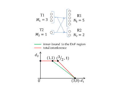
Figure 1: An Example of the IC with Asymmetrically Constrained Transmitters

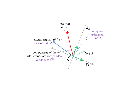
Figure 2: The Receive Signal-Space of R2 with Uniform Signaling at T1

To understand this, let us consider an example of the IC with $(M_{1},M_{2},N_{1},N_{2})=(3,1,5,2)$ (see Fig. 1) and focus on the case of $d_{2}=1$. The inequality in (3) reduces to

$$f\big{(}~{}I(\mathbf{X^{1}};\mathbf{Z}|M_{Z},\mathbf{H})~{}\big{)}\leq 1.$$ (5)

Consider a particular transmission scheme which satisfies the above inequality. Suppose T1 transmits $3$ data symbols that are i.i.d. according to $\mathcal{C}\mathcal{N}(0,P^{\alpha})$, $0<\alpha\leq\frac{1}{2}$ (we refer to such signaling as uniform signaling); T2 transmits a $\mathcal{C}\mathcal{N}(0,P)$ data symbol; and the signals of T1 and T2 are i.i.d. across time. It is not difficult to prove that such a strategy satisfies the inequality in (5) (with equality if $\alpha=\frac{1}{2}$). Moreover, R1 has sufficient number of antennas to zero-force the interference and achieve up to $3\alpha\leq\frac{3}{2}$ DoF. Now consider the receive signal-space of R2 shown in Fig. 2 where, for simplicity, we take $b=1$ and time index $t$ is shown explicitly. With uniform signaling at T1, the interference $H^{21}(t)X^{1}(t)$ at R2 satisfies the following properties:

1. If we pick any $2$ orthonormal basis vectors for the $2$-dimensional receive signal space of R2, then the components of the interference along the two basis vectors are independent and each has a variance of $P^{\alpha}$; and

2. any $1$-dimensional subspace chosen in the $2$-dimensional receive signal space of R2 carries a component of the interference with multiplexing gain equal to $\alpha$ (since its variance is $P^{\alpha}$).

Further, the useful signal $H^{22}(t)X^{2}(t)$ can span only a $1$-dimensional subspace since $M_{2}=1$. Hence, the subspace orthogonal to the span of $H^{22}(t)$ can not give any information to R2 about the useful signal $X^{2}(t)$. In other words, out of the total $2$ DoF available to R2, $1$ DoF is lost because T2 has just $M_{2}=1(<2=N_{2})$ antenna. Moreover, out of the $1$ DoF that is left at R2, $\alpha$ DoF are occupied by the interference (see Property (b) of the interference at R2). Thus, R2 has only $1-\alpha$ DoF available for decoding the useful signal so that it can not achieve $d_{2}=1$. Hence the claim of (4) is true.

We next argue through the same example that the claim of (4) holds because $M_{2}<N_{2}$. Now, R2 can not achieve $d_{2}=1$ since the $1$ DoF available to it is lost due to the limitation at T2 that its transmit signal can not span the entire receive signal space. In particular, had this limitation not existed such as when $M_{2}=2$ (with $M_{1}$, $N_{1}$, and $N_{2}$ unchanged), R2 would have been able to achieve $d_{2}=1$. To see this, note that T2 in this case can transmit two complex Gaussian symbols each with a power of $\frac{P}{2}$ and make $X^{2}(t)$ span the entire receive signal space enabling R2 to achieve $d_{2}=1$ by treating interference as noise, even if T1 employs uniform signalling (note R1 can still zero-force the interference to successfully recover the useful signal). Therefore, we conclude that the claim in (4) holds because $M_{2}<N_{2}$. Hence the implication in (3) is insufficient in the sense that it does not capture the further limitation imposed by $M_{2}<N_{2}$.

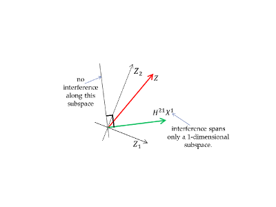
Figure 3: Interference Localization at R2

Indeed, for ICs with asymmetrically constrained transmitters, we must constrain how the interference is distributed in the receive signal-space of R2 in addition to upper-bounding its multiplexing gain using the inequality of (4). This is explained in the context of our example. It must be proved that if $d_{2}=1$ is achievable then the interference $H^{21}(t)X^{1}(t)$ spans a $1$-dimensional subspace at R2, or there exists a subspace which does not contain any interference (with positive multiplexing gain), see Fig. 3. This is because if this were not true, then, as argued for the case where T1 employs uniform signaling, $d_{2}=1$ can not be achieved. In other words, we must prove that if $d_{2}=1$ is achievable, then the interference is localized to a smaller-dimensional subspace and it cannot be distributed uniformly in the receive signal-space of R2, which is the case if T1 employs uniform signaling.

In general, it must be shown that if $d_{2}$ DoF are achievable for T2-R2 pair over an IC with asymmetrically constrained transmitters, then the interference $H^{21}(t)X^{1}(t)$ at R2 must be such that

1. its multiplexing gain is at most $N_{2}-d_{2}$ (as required by the inequality in (4)); and additionally,

2. there exists an $M_{2}$-dimensional subspace in the receive signal-space of R2 that carries interference with multiplexing gain at most $M_{2}-d_{2}$.

We call this property interference localization, because at $d_{2}=M_{2}$, it amounts to the entire interference being localized to some $(N_{2}-M_{2})$-dimensional subspace. Our intuition suggests that if this property is proved, we would get the tightest characterization of the DoF region. Indeed, Lemma 2 of the next sub-section accomplishes this task, using which the desired bound $L$ is derived.

III-B Main Proof

We prove here that for the MIMO IC with asymmetrically constrained transmitters, $L$ with $N_{1}^{\prime}=\min(M_{1},N_{1})$ is an outer-bound. To this end, first obtain the singular-value decomposition of the isotropically-distributed channel matrices.

Lemma 1

For an $N_{i}\times M_{j}$ isotropically-distributed channel matrix $H^{ij}(t)$, we may write

$$H^{ij}(t)=U^{ij}(t)\Lambda^{ij}(t)\big{(}V^{ij}(t)\big{)}^{*},$$

where $U^{ij}(t)$, $\Lambda^{ij}(t)$, and $V^{ij}(t)$ are deterministic functions of $H^{ij}(t)$ such that

1. $U^{ij}(t)$ is an $N_{i}\times N_{i}$ unitary matrix;

2. $\Lambda^{ij}(t)$ is an $N_{i}\times\min(N_{i},M_{j})$ diagonal matrix containing the singular values of $H^{ij}(t)$, i.e., the square matrix formed by retaining its first $\min(N_{i},M_{j})$ rows, denoted henceforth as $\tilde{\Lambda}^{ij}(t)$, is diagonal with singular values of $H^{ij}(t)$ along its diagonal and the remaining rows consist only of zeros;

3. $V^{ij}(t)$ is an $M_{j}\times\min(N_{i},M_{j})$ isotropically-distributed semi-unitary matrix, i.e., $\big{(}V^{ij}(t)\big{)}^{*}V^{ij}(t)=I_{\min(N_{i},M_{j})}$ and it is uniformly distributed over its domain; and

4. $V^{ij}(t)$ is independent of $U^{ij}(t)$ and $\Lambda^{ij}(t)$.

Proof:

Follows from [4, Lemma 1]. ∎

To explain the main idea, we first consider the case where $U^{11}(t)=I_{N_{1}}$, $U^{21}(t)=I_{N_{2}}(t)$, and all singular values of $H^{11}(t)$ and $H^{21}(t)$ are equal to unity with probability $1$. These assumptions about $U^{i1}(t)$ and $\Lambda^{i1}(t)$ will be in effect until the general case is discussed towards the end. Note that under these assumptions $\Lambda^{21}(t)=I_{N_{2}}$ since $N_{2}<M_{1}$.

The proof now consists of three steps.
$\bullet$ Step I: Use Fano’s inequality to bound $d_{2}$. It is argued that this bound can not immediately be used to obtain the desired bound $L$, which motivates the analysis of the next step.
$\bullet$ Step II: Obtain tight bounds on the interference at R2 by proving interference localization.
$\bullet$ Step III: Apply Fano’s inequality to bound $d_{1}$ in terms of the multiplexing gain of a certain mutual information term (see equation (14)), which is then upper-bounded using the bounds derived at Step II.

Step I: We apply Fano’s inequality [7] at R2 to obtain

$$bR_{2}\leq I(M_{Z};\mathbf{Z}|\mathbf{H})+b\epsilon_{b},$$ (6)

where $b$ is the bocklength and $\epsilon_{b}\to 0$ as $b\to\infty$. This yields

$$bR_{2} \leq I(M_{Y},M_{Z};\mathbf{Z}|\mathbf{H})-I(M_{Y};\mathbf{Z}|M_{Z},\mathbf{H})+b\epsilon_{b}$$

$$\Rightarrow bR_{2} + I(M_{Y};\mathbf{Z}|M_{Z},\mathbf{H})\leq I(M_{Y},M_{Z};\mathbf{Z}|\mathbf{H})+b\epsilon_{b}.$$ (7)

Now, if $(d_{1},d_{2})\in\mathbf{D}_{\rm{IC}}$, then, by definition, there exists a sequence $\big{(}R_{1}(P),R_{2}(P)\big{)}\in\mathcal{C}(P)$ such that $d_{2}=\lim_{P\to\infty}\frac{1}{\log_{2}P}\lim_{b\to\infty}\frac{bR_{2}}{b}$. Moreover, for any rate pair $\big{(}R_{1}(P),R_{2}(P)\big{)}\in\mathcal{C}(P)$, $R_{2}(P)\equiv R_{2}$ satisfies inequality (7). Therefore, from (7), we get

$$d_{2}+f\big{(}~{}I(M_{Y};\mathbf{Z}|M_{Z},\mathbf{H})~{}\big{)} \leq f\Big{(}bR_{2}+I(M_{Y};\mathbf{Z}|M_{Z},\mathbf{H})\Big{)}$$

$$\leq f\Big{(}I(M_{Y},M_{Z};\mathbf{Z}|\mathbf{H})+b\epsilon_{b}\Big{)}$$

$$= f\Big{(}I(M_{Y},M_{Z};\mathbf{Z}|\mathbf{H})\Big{)}$$

$$\Rightarrow d_{2}\leq N_{2} - f\big{(}~{}I(M_{Y};\mathbf{Z}|M_{Z},\mathbf{H})~{}\big{)},$$ (8)

where the last inequality holds due to the single-user bound. Here, the number $f\big{(}I(M_{Y};\mathbf{Z}|M_{Z},\mathbf{H})\big{)}$ is equal to the multiplexing gain of the net (per unit time) interference encountered by R2; and the above inequality constrains the multiplexing gain of the total interference seen by R2 per unit time. However, as explained in the last sub-section, this inequality does not completely capture the limitation of the second transmit-receive pair due to $M_{2}<N_{2}$. As per the discussion therein, we must prove an additional bound that constrains how the interference is distributed. Such bounds are derived in the following lemma.

Step II:

Lemma 2 (Interference Localization)

We have

$$f\big{(}~{}I(M_{Y};~{}\mathbf{Z}_{[1:M_{2}]}~{}\big{|}M_{Z},~{}\mathbf{Z}_{[M_{2}+1:N_{2}]},~{}\mathbf{H})~{}\big{)}\leq M_{2}-d_{2},$$ (9)

$${\rm and}\quad f\big{(}~{}I(M_{Y};~{}\mathbf{Z}_{[M_{2}+1:N_{2}]}~{}\big{|}M_{Z},~{}\mathbf{H})~{}\big{)}\leq N_{2}-M_{2}.$$ (10)

Note that the bound in (8) can be recovered by simply adding inequalities (9) and (10), and therefore, these two bounds are tighter than the one in (8). Moreover, these bounds assert that if $d_{2}$ DoF are achievable for the second transmit-receive pair, then there exists an $M_{2}$-dimensional subspace (of the receive signal-space of R2), which carries interference with multiplexing gain at most $M_{2}-d_{2}$. Thus, these bounds capture the notion of interference localization.

We now prove the above lemma.

Proof:

Let $\tilde{Z}(t)\stackrel{{\scriptstyle\triangle}}{{=}}\big{(}U^{22}(t)\big{)}^{*}Z(t)$. Since $\big{(}U^{22}(t)\big{)}^{*}H^{22}(t)=\Lambda^{22}(t)\big{(}V^{22}(t)\big{)}^{*}$, where $\Lambda^{22}(t)$ is diagonal with the bottom $N_{2}-M_{2}$ rows containing only zeros, we observe that the transmit signal $X^{2}(t)$ can not affect the last $N_{2}-M_{2}$ elements of $\tilde{Z}(t)$ $\forall$ $t$. In other words, $\mathbf{\tilde{Z}}_{[M_{2}+1:N_{2}]}$ is independent of $M_{Z}$, which yields

$$~{}bR_{2}\leq I\big{(}M_{Z}~{};~{}\mathbf{Z}~{}\big{|}~{}\mathbf{H}\big{)}+b\epsilon_{b}=I\big{(}M_{Z}~{};~{}\mathbf{\tilde{Z}}~{}\big{|}~{}\mathbf{H}\big{)}+\epsilon_{b}$$

$${}=I\big{(}M_{Z}~{};~{}\mathbf{\tilde{Z}}_{[1:M_{2}]}~{}\big{|}~{}\mathbf{\tilde{Z}}_{[M_{2}+1:N_{2}]},~{}\mathbf{H}\big{)}+b\epsilon_{b}$$

$${}\hskip 17.07182pt+I\big{(}M_{Z}~{};~{}\mathbf{\tilde{Z}}_{[M_{2}+1:N_{2}]}~{}\big{|}~{}\mathbf{H}\big{)}$$

$${}=I\big{(}M_{Z}~{};~{}\mathbf{\tilde{Z}}_{[1:M_{2}]}~{}\big{|}~{}\mathbf{\tilde{Z}}_{[M_{2}+1:N_{2}]},~{}\mathbf{H}\big{)}+b\epsilon_{b}$$

Now, the techniques developed for deriving inequality (8) from (III-B) can be used to obtain

$$f\Big{(}I(M_{Y};~{}\mathbf{\tilde{Z}}_{[1:M_{2}]}~{}\big{|}M_{Z},~{}\mathbf{\tilde{Z}}_{[M_{2}+1:N_{2}]},~{}\mathbf{H})\Big{)}\leq M_{2}-d_{2}.$$ (11)

Moreover, by the single-user bound, we have

$$f\Big{(}I(M_{Y};\mathbf{\tilde{Z}}_{[M_{2}+1:N_{2}]}~{}\big{|}M_{Z},\mathbf{H})\Big{)}\leq N_{2}-M_{2}.$$ (12)

Note that conditioned on $M_{Z}$, $X^{2}(t)$ is deterministic. Since translation does not change differential entropy, it may be assumed that $X^{2}(t)=0$ $\forall$ $t$ (see [3, Proof of Lemma 2] for detailed proof). Thus, we may compute the mutual information terms in (11) and (12) by taking

$$\tilde{Z}(t)=\big{(}U^{22}(t)\big{)}^{*}H^{21}(t)X^{1}(t)+\big{(}U^{22}(t)\big{)}^{*}W^{\prime}(t).$$

Further, note that $U^{22}(t)$, being a function of $H^{22}(t)$, is independent of $H^{21}(t)$. Since we have assumed here that $U^{21}(t)=I_{N_{2}}$ and $\Lambda^{21}(t)=I_{N_{2}}$, we have $\big{(}U^{22}(t)\big{)}^{*}H^{21}(t)=\big{(}U^{22}(t)\big{)}^{*}\big{(}V^{21}(t)\big{)}^{*}$. For any unitary matrix $U^{22}(t)$, it can be easily shown that $V^{21}(t)U^{22}(t)$ is still a semi-unitary matrix that is uniformly distributed over its domain. This implies that $V^{21}(t)$ is identically distributed as $V^{21}(t)U^{22}(t)$, which we denote symbolically as $V^{21}(t)\sim V^{21}(t)U^{22}(t)$. Moreover, $W^{\prime}(t)\sim\big{(}U^{22}(t)\big{)}^{*}W^{\prime}(t)$. Hence, conditioned on $M_{Z}$ and $\mathbf{H}$, $Z(t)\sim\tilde{Z}(t)$ or $\mathbf{Z}\sim\mathbf{\tilde{Z}}$. Hence, we get the lemma from bounds (11) and (12). ∎

Step III: This is the final step of the analysis. Consider R1. Assuming that it knows message $M_{Z}$, we get via Fano’s inequality that

$$bR_{1} \leq I(M_{Y};\mathbf{Y}|M_{Z},\mathbf{H})+b\epsilon_{b}$$ (13)

$$\Rightarrow d_{1} \leq f\big{(}I(M_{Y};\mathbf{Y}|M_{Z},\mathbf{H})\big{)}.$$ (14)

Since conditioned on $M_{Z}$, $X_{2}(t)$ can be taken to be equal to $0$ $\forall$ $t$, $U^{i1}(t)$ has been assumed to be equal to $I_{N_{1}}$, and $\Lambda^{i1}(t)$ is diagonal, we observe that if $N_{1}>M_{1}$, the last $N_{1}-M_{1}$ antennas of R1 receive only noise at all times. Therefore, the random variables $\mathbf{Y}_{M_{1}+1:N_{1}}$ can be ignored in $f\big{(}I(M_{Y}~{};~{}\mathbf{Y}~{}\big{|}~{}M_{Z},\mathbf{H})\big{)}$, which upper-bounds $d_{1}$ in (14). Thus, henceforth in this section, it is assumed that $N_{1}=N_{1}^{\prime}=\min(N_{1},M_{1})$.

$$\bar{Y}(t) \stackrel{{\scriptstyle\triangle}}{{=}} h^{1}_{\max}(t)\big{(}D^{11}(t)\big{)}^{-1}\big{(}U^{11}(t)\big{)}^{*}\begin{bmatrix}H^{11}(t)&H^{12}(t)\end{bmatrix}\begin{bmatrix}X^{1}(t)\\ X^{2}(t)\end{bmatrix}+W(t),\mbox{ where }D^{11}(t)=\begin{bmatrix}\tilde{\Lambda}^{11}(t)&0_{p_{1}\times q_{1}}\\ 0_{q_{1}\times p_{1}}&I_{q_{1}\times q_{1}}\end{bmatrix}.\!\!$$ (15)

$$\bar{Z}(t) \stackrel{{\scriptstyle\triangle}}{{=}} h^{1}_{\max}(t)\big{(}\Lambda^{21}(t)\big{)}^{-1}\big{(}U^{21}(t)\big{)}^{*}\big{\{}H^{21}(t)X^{1}(t)+H^{22}(t)X^{2}(t)\big{\}}+W^{\prime}(t).\!\!$$ (16)

$$\overline{\mathbf{D}}_{\rm{IC\backslash CRC}}\stackrel{{\scriptstyle\triangle}}{{=}}\left\{(d_{1},d_{2})\in\mathbb{R}^{2}_{+}\Big{|}\forall~{}(w_{1},w_{2})\in\mathbb{R}^{2}_{+},~{}w_{1}d_{1}+w_{2}d_{2}\leq\overline{\lim_{P\to\infty}}~{}\frac{1}{\log_{2}P}\left[\sup_{\big{(}R_{1}(P),R_{2}(P)\big{)}\in\mathcal{C}(P)}\Big{\{}w_{1}R_{1}+w_{2}R_{2}\Big{\}}\right]\right\}.$$ (17)

We now divide the antennas of R1 into two groups: the first group consists of the last $l\stackrel{{\scriptstyle\triangle}}{{=}}N_{2}-M_{2}$ antennas of R1, while the second group contains the remaining $N_{1}-l$ antennas. Then, using the chain rule for the mutual information [7], we get

$$d_{1}\leq f\big{(}I(M_{Y}~{};~{}\mathbf{Y}~{}\big{|}~{}M_{Z},\mathbf{H})\big{)}~{}\quad\mbox{ with }N_{1}=N_{1}^{\prime}$$

$${}=f\big{(}I(M_{Y}~{};~{}\mathbf{Y}_{[N_{1}-l+1:N_{1}]}~{}\big{|}~{}M_{Z},~{}\mathbf{H})\big{)}$$

$${}+f\big{(}I(M_{Y}~{};~{}\mathbf{Y}_{[1:N_{1}-l]}~{}\big{|}~{}M_{Z},~{}\mathbf{Y}_{[N_{1}-l+1:N_{1}]},~{}\mathbf{H})\big{)}.$$

We bound each of the two terms appearing in (III-B) starting with the first term. Toward this end, note that the isotropicity of the channel matrices and the assumptions made about $U^{i1}(t)$ and $\Lambda^{i1}(t)$ together imply that for any given $b$, the joint distribution of the random variables $\mathbf{Y}_{[N_{1}-l+1:N_{1}]}$, conditioned on $M_{Z}$ and $\mathbf{H}$, is identical to that of $\mathbf{Z}_{[M_{2}+1:N_{2}]}$, conditioned on $M_{Z}$ and $\mathbf{H}$. Hence,

$$f\big{(}I(M_{Y}~{};~{}\mathbf{Y}_{[N_{1}-l+1:N_{1}]}~{}\big{|}~{}M_{Z},~{}\mathbf{H})\big{)}$$ (19)

$${}=f\big{(}I(M_{Y};~{}\mathbf{Z}_{[M_{2}+1:N_{2}]}~{}\big{|}M_{Z},~{}\mathbf{H})\big{)}\leq N_{2}-M_{2}.$$

For the second term in (III-B), we have the following lemma.

Lemma 3

If $l=N_{2}-M_{2}$, then

$$f\big{(}I(M_{Y}~{};~{}\mathbf{Y}_{[1:N_{1}-l]}~{}\big{|}~{}M_{Z},~{}\mathbf{Y}_{[N_{1}-l+1:N_{1}]},~{}\mathbf{H})\big{)}$$ (21)

$${}\leq\frac{N_{1}-l}{M_{2}}f\big{(}I(M_{Y};~{}\mathbf{Z}_{[1:M_{2}]}~{}\big{|}M_{Z},~{}\mathbf{Z}_{[M_{2}+1:N_{2}]},~{}\mathbf{H})\big{)}$$

$${}\leq\frac{N_{1}+M_{2}-N_{2}}{M_{2}}(M_{2}-d_{2}).$$

Proof:

The last inequality follows from the definition of $l$ and inequality (9). Hence, it is sufficient to prove the first inequality, which is done in Appendix A. ∎

Substituting the inequalities (19) and (21) into (III-B), we get

$$d_{1}\leq N_{2}-M_{2}+\frac{N_{1}+M_{2}-N_{2}}{M_{2}}(M_{2}-d_{2})$$

$${}\Rightarrow d_{1}+\frac{N_{1}+M_{2}-N_{2}}{M_{2}}d_{2}\leq N_{1},$$

which is the desired inequality since $N_{1}=N_{1}^{\prime}$.

The general case without any assumptions about $U^{i1}(t)$ and $\Lambda^{i1}(t)$: While this case follows from the techniques developed in [3, Appendix D], we include the details for the sake of completeness. We manipulate $Y(t)$ and $Z(t)$ to define $\bar{Y}(t)$ and $\bar{Z}(t)$ such that the mutual information terms in equations (13) and (6) are upper-bounded and the proof presented above holds if $\bar{Y}(t)$ and $\bar{Z}(t)$ are considered as the channel outputs. To this end, define $h(t)$ to be the maximum of all elements of matrices $\Lambda^{11}(t)$ and $\Lambda^{21}(t)$. Define $h^{1}_{\max}(t)=\max\{1,h(t)\}$. Further, $p_{1}\stackrel{{\scriptstyle\triangle}}{{=}}\min(M_{1},N_{1})$, $q_{1}\stackrel{{\scriptstyle\triangle}}{{=}}N_{1}-p_{1}$. Recall that $\Lambda^{21}(t)$ is square to define $\bar{Y}(t)$ and $\bar{Z}(t)$ in equations (15) and (16) at the bottom the page. It can be proved that $I(M_{Y};\mathbf{Y}|M_{Z},\mathbf{H})\leq I(M_{Y};\mathbf{\bar{Y}}|M_{Z},\mathbf{H})$ and $I(M_{Z};\mathbf{Z}|\mathbf{H})\leq I(M_{Z};\mathbf{\bar{Z}}|\mathbf{H})$ (see proofs of Theorems 5 and 6 from [3]). Define $\bar{H}^{11}(t)$ and $\bar{H}^{12}(t)$ such that $\bar{Y}(t)=\bar{H}^{11}(t)X^{1}(t)+\bar{H}^{12}(t)X^{2}(t)+W(t)$ and analogously $\bar{H}^{21}(t)$ and $\bar{H}^{22}(t)$. Now the proof given above applies by making the following correspondence: $Y(t)\leftrightarrow\bar{Y}(t)$, $Z(t)\leftrightarrow\bar{Z}(t)$, and $H^{ij}(t)\leftrightarrow\bar{H}^{ij}(t)$ $\forall$ $i,j,t$.

III-C Comparison with the Proof of [4]

Interference localization is central to the above proof as well as to the one in [4]. However, the two works employ completely different techniques to prove this fact. In [4], the authors first assume that R1 knows the message $M_{Z}$ (as we do here), and under this assumption, show that, as far as the DoF region is concerned, it is optimal for T2 to transmit $X^{2}(t)$ that is Gaussian with distribution $\mathcal{C}\mathcal{N}(0,\frac{P}{M_{2}}I_{M_{2}})$ (see Theorem 3 therein). Subsequently, for $X^{2}\sim\mathcal{C}\mathcal{N}(0,\frac{P}{M_{2}}I_{M_{2}})$, it is proven using a lemma (namely, Lemma 4 therein) that the subspace spanned by $X^{2}(t)$ at R2 can not provide any information to it about the transmit signal $X^{1}(t)$ (cf. equation (47) therein), which in a way captures the interference localization phenomenon. In contrast, we prove here the same point in Lemma 2 using basic information-theoretic identities like the chain rule for mutual information [7].

Another important step in our proof is Lemma 3, which again follows from simple identities such as conditioning reduces entropy, the chain rule for differential entropy, etc. On the other hand, the proof in [4] needs a result (namely, Lemma 3 therein) that is a counterpart of Lemma 3 we have here, its proof is given there using more involved techniques which invoke the minimum mean squared error (MMSE). The proof here, in addition to be being simpler, is also more widely applicable, as we illustrate below.

We use the bounding techniques developed in this section to obtain the no-CSIT DoF region of the CRC with asymmetrically constrained transmitters (see Theorems 2 and 4) for which the inner and outer-bounds (to the no-CSIT DoF region) reported in [3] are not tight. However, the extension to this problem of the technique of [4] is not known because their approach rests critically on being able to prove the optimality of choosing $X^{2}(t)$ to be Gaussian, which, in the context of the CRC, may not hold since T2 is now transmitting not just to R2 but also to R1.

Further, consider the problem of determining the generalized DoF (GDoF) region of the no-CSIT IC, where the GDoF region is defined to be equal to the DoF region when the gains (i.e., the Frobenius norm [14]) of the direct-link channel matrices ($H^{11}(t)$ and $H^{21}(t)$) and those of the cross-link channel matrices ($H^{12}(t)$ and $H^{22}(t)$) are unequal with the ratio of their values in dB equal to $\alpha\geq 0$ (the DoF region is the GDoF with $\alpha=1$; see [10] for a formal definition). It turns out that for characterizing the no-CSIT GDoF region of the IC with asymmetrically constrained transmitters in the very weak interference regime of $\alpha\leq\frac{1}{2}$, it is necessary to prove that the interference is localized which, even in the more general setting of the GDoF analysis, can be done using the techniques developed above [9]. In contrast, however, the applicability of the approach of [4] is not clear (cf. [9]). This is because for small values of $\alpha$, the bound obtained by assuming that R1 knows the message $M_{Z}$ is loose (since R1 at low $\alpha$ can not possibly decode $M_{Z}$, cf. [10, Subsections III-C and III-D]). Hence, an outer-bound must be derived without assuming R1 to know the message $M_{Z}$, in which case the optimality of choosing $X^{2}(t)$ to be Gaussian (with a certain covariance matrix) can not be shown.

III-D The More General Definition

As stated earlier, the definition of $\mathbf{D}_{\rm{IC\backslash CRC}}$ in (II) is restrictive. Here we define the DoF region (cf. [12]) more generally (by relaxing the requirement that the limits $\lim_{P\to\infty}\frac{R_{i}(P)}{\log_{2}P}$, $i=1,2$ exist) to be the region $\overline{\mathbf{D}}_{\rm{IC\backslash CRC}}$ in equation (17) at the bottom of the previous page, where $\mathbb{R}_{+}$ denotes the set of non-negative real numbers. Comparing the two definitions, we have

$$\mathbf{D}_{\rm{IC\backslash CRC}}\subseteq\overline{\mathbf{D}}_{\rm{IC\backslash CRC}}$$

The techniques developed in the earlier part of this section allow us to characterize $\overline{\mathbf{D}}_{\rm{IC}}$ as per the following theorem.

Theorem 5

With no CSIT, we have for the MIMO IC with isotropic fading and for the MIMO CRC with i.i.d. (or correlated) Rayleigh fading, we have

$$\overline{\mathbf{D}}_{\rm{IC\backslash CRC}}=\mathbf{D}_{\rm{IC\backslash CRC}}$$

Proof:

For the MIMO IC, it is sufficient to prove that if $(d_{1},d_{2})\in\overline{\mathbf{D}}_{\rm{IC}}$, then the bound $L$

$$d_{1}+\frac{N_{1}^{\prime}+M_{2}-N_{2}}{M_{2}}d_{2}\leq N_{1}^{\prime}$$

holds with $N_{1}^{\prime}=\min(M_{1},N_{1})$. See Appendix B. The DoF region $\overline{\mathbf{D}}_{\rm{CRC}}$ can be shown to coincide with $\mathbf{D}_{\rm{CRC}}$ determined in Theorems 2 and 4 for i.i.d. and correlated Rayleigh fading cases, respectively, in an analogous manner. ∎

IV Proof of Theorem 2: $L$ is an Outer-Bound

The goal of this section is to show that for the MIMO CRC with asymmetrically constrained transmitters and i.i.d. Rayleigh fading, bound $L$ is an outer-bound with $N_{1}^{\prime}=\min(M_{1}+M_{2},N_{1})$. In the following sub-section, we first deal with the case of $N_{1}\geq M_{1}+M_{2}$; later, in Section IV-B, we address the remaining case of $N_{1}<M_{1}+M_{2}$.

IV-A Case of $N_{1}\geq M_{1}+M_{2}$

The proof again consists of three steps, as was the case in the last section. At Step I, we bound $d_{1}$. At Step II, derive the interference localization property; and at Step III, bound $d_{1}$.

Step I: Fano’s inequality yields us

$$bR_{2}\leq I\big{(}M_{Z};\mathbf{Z}\big{|}\mathbf{H}\big{)}+b\epsilon_{b}.$$ (22)

Step II: To prove that the interference is localized at R2, we make use of the following lemma, which gives us the QR-decomposition [14] of $H^{22}(t)$.

Lemma 4

An i.i.d. Rayleigh-faded $N_{2}\times M_{2}$ channel matrix $H^{22}(t)$ can be written as

$$H^{22}(t)=Q^{22}(t)R^{22}(t),$$

where $Q^{22}(t)$ and $R^{22}(t)$ are deterministic functions of $H^{22}(t)$ such that

1. $Q^{22}(t)$ is an $N_{2}\times N_{2}$ isotropically-distributed unitary matrix;

2. $R^{22}(t)$ is an $N_{2}\times M_{2}$ upper-triangular matrix, i.e., the $M_{2}\times M_{2}$ square matrix formed by retaining just the first $M_{2}$ rows of it is upper-triangular, while the bottom $N_{2}-M_{2}$ rows of it consist only of zeros;

3. entries of $R^{22}(t)$, which are not surely zero, follow a continuous distribution (i.e., their cumulative distribution function is continuous and differentiable); and

4. all entries of $R^{22}(t)$ are independent of each other and also of the unitary matrix $Q^{22}(t)$.

Proof:

Follows from the definition of QR-decomposition [14] and [15, Lemma 2.1]. ∎

With $Q^{22}(t)$ and $R^{22}(t)$ obtained as per the above lemma, define

$$\tilde{Z}(t)\stackrel{{\scriptstyle\triangle}}{{=}}\big{(}Q^{22}(t)\big{)}^{*}Z(t).$$ (23)

This construction allows us to obtain the following lemma.

Lemma 5 (Interference Localization)

The following bounds hold:

$$f\big{(}I(M_{Y};\mathbf{\tilde{Z}}_{[1:M_{2}]}~{}\big{|}M_{Z},\mathbf{\tilde{Z}}_{[M_{2}+1:N_{2}]},\mathbf{H})\big{)} \leq M_{2}-d_{2},$$ (24)

$$\mbox{and}~{}f\big{(}I(M_{Y};\mathbf{\tilde{Z}}_{[M_{2}+1:N_{2}]}~{}\big{|}M_{Z},\mathbf{H})\big{)} \leq N_{2}-M_{2}.$$ (25)

Proof:

Since the bottom $N_{2}-M_{2}$ entries of $R^{22}(t)$ consist only of zeros, the transmit signal $X^{2}(t)$ can not affect the last $N_{2}-M_{2}$ entries of $\tilde{Z}(t)$. Moreover, the signal $X^{1}(t)$ is independent of $M_{Z}$. This observation and the analysis in the proof of Lemma 2 up to equations (11) and (12) allow us to derive the inequalities of the lemma. ∎

Recall, in the previous section, we were able to claim that the above bounds hold even with $\mathbf{\tilde{Z}}$ replaced by $\mathbf{Z}$ because in the case of the IC, conditioned on $M_{Z}$, $X^{2}(t)$ can be taken to be deterministic. However, this need not be the case with the CRC where T2 knows both the messages. As a result, in the present case, the above bounds do not hold with $\mathbf{\tilde{Z}}$ replaced by $\mathbf{Z}$. This necessitates a more sophisticated analysis at Step III for the CRC.

Before proceeding further, we state a corollary which simplifies the computation of the mutual information terms appearing in the above two equations.

Corollary 1

In the mutual information terms appearing in inequalities (24) and (25), it may be assumed that $\mathbf{\tilde{Z}}=\big{\{}\tilde{Z}(t)\big{\}}_{t=1}^{b}$, where

$$\tilde{Z}(t)=H^{21}(t)X^{1}(t)+R^{22}(t)X^{2}(t)+W^{\prime}(t).$$ (26)

Proof:

See Appendix C-A. ∎

Thus, henceforth, we assume that equation (26) holds and $\tilde{Z}(t)$ is treated as the signal received by R2.

Step III: Consider now R1. Assuming that it knows $M_{Z}$, we get via Fano’s inequality that

$$d_{1}\leq f\big{(}I(M_{Y};\mathbf{Y}\big{|}M_{Z},\mathbf{H})\big{)}.$$ (27)

Suppose $N_{1}>M_{1}+M_{2}$. Then, at any given $t$, R1 can construct a noisy version of the channel inputs $X^{1}(t)$ and $X^{2}(t)$ using just $M_{1}+M_{2}$ channel outputs $Y_{[1:M_{1}+M_{2}]}(t)$ by inverting a matrix

$$\begin{bmatrix}H^{11}_{[1:M_{1}+M_{2}]}(t)&H^{12}_{[1:M_{1}+M_{2}]}(t)\end{bmatrix},$$

(which can be done with probability $1$). Hence, the last $N_{1}-(M_{1}+M_{2})$ channel outputs at R1 can not contribute to the DoF of the CRC, and therefore, they can be ignored in the present analysis (see [3, Section II-C] for detailed proof of this claim). It is thus assumed in this sub-section that $N_{1}\leq M_{1}+M_{2}$ and $N_{1}^{\prime}=N_{1}$.

We would like to use the inequalities (24) and (25) to bound the term $f\big{(}I(M_{Y};\mathbf{Y}\big{|}M_{Z},\mathbf{H})\big{)}$. However, the channel matrices $H^{11}(t)$ and $H^{12}(t)$ corresponding to R1 are i.i.d. Rayleigh faded, while those corresponding to R2 (which observes $\tilde{Z}(t)$) are not (see equation (26)). As a result, the inequalities (24) and (25) can not directly be used to bound $f\big{(}I(M_{Y};\mathbf{Y}\big{|}M_{Z},\mathbf{H})\big{)}$. Instead, we first need to manipulate this term to bring it to a form that is suitable for the application of bounds in (24) and (25).

The analysis henceforth is divided into four steps, namely, Steps III.a - III.d. Before getting into the details of these steps, we explain below the outline since the analysis is complicated. This outline has also been depicted in Table I in the context of the CRC with $(M_{1},M_{2},N_{1},N_{2})=(5,2,7,3)$.

$\bullet$ Step III.a: At this step, we upper-bound the mutual information term $I(M_{Y};\mathbf{Y}\big{|}M_{Z},\mathbf{H})$ by assuming that R1, at time $t$, observes not just the actual channel outputs $Y_{i}(t)$, $i\in[1:N_{1}]$, but also some extra fictitious channel outputs which are defined shortly. See Step III.a in Table I). The fictitious outputs are added such that we have $N_{2}$ outputs $Y_{S_{i}}$ corresponding to each set $S_{i}$ and $Y_{S_{i}}(t)\sim Z(t)$.

$\bullet$ Step III.b: Here, we use the QR-decomposition of Lemma 4 to transform the outputs $Y_{S_{i}}(t)$ into $\tilde{Y}_{S_{i}}(t)$ such that $\tilde{Y}_{S_{i}}(t)\sim\tilde{Z}(t)$.

$\bullet$ Step III.c: It is shown that the upper-bound on $d_{1}$ obtained at Step III.b can be tightened by suitably removing some of the entries of $\tilde{Y}_{S_{i}}$. See Step III.c in Table I.

$\bullet$ Step III.d: This is the final step at which the bounds (24), (25), and the one obtained at Step III.c are used to derive the desired bound $L$.

We now proceed to the proof.

To begin, we bound $d_{1}$ via Fano’s inequality as

$$d_{1}\leq f\Big{(}~{}I\big{(}M_{Y};\mathbf{Y}\Big{|}M_{Z},\mathbf{H}\big{)}~{}\Big{)}.$$

The proof now proceeds through the following four steps.

Step III.a : Group the actual channel outputs into $4$ sets and add fictitious channel outputs so that each set contain $N_{2}=3$ outputs.

Set	indices	Actual Outputs
$S_{1}^{a}$	$\{1\}$	$Y_{1}$
$S_{2}^{a}$	$\{2\}$	$Y_{2}$
$S_{3}^{a}$	$\{3,4\}$	$Y_{3},\>Y_{4}$
$S_{0}^{a}$	$\{5,6,7\}$	$Y_{5},\>Y_{6},\>Y_{7}$

(a)

Set	indices	Fictitious outputs
$S_{1}^{f}$	$\{f11,\>f12\}$	$Y_{f11},\>Y_{f12}$
$S_{2}^{f}$	$\{f21,\>f22\}$	$Y_{f21},\>Y_{f22}$
$S_{3}^{f}$	$\{f31\}$	$Y_{f31}$
$S_{0}^{f}$	$\{\phi\}$	$\phi$

(b)

Set	indices	All Outputs
$S_{1}=S_{1}^{a}\cup S_{1}^{f}$	$\{1,\>f11,\>f12\}$	$Y_{S_{1}}=\{Y_{1},\>Y_{f11},\>Y_{f12}\}$
$S_{2}=S_{2}^{a}\cup S_{2}^{f}$	$\{2,\>f21,\>f22\}$	$Y_{S_{2}}=\{Y_{2},\>Y_{f21},\>Y_{f22}\}$
$S_{3}=S_{3}^{a}\cup S_{3}^{f}$	$\{3,\>4,\>f31\}$	$Y_{S_{3}}=\{Y_{3},\>Y_{4},\>Y_{f31}\}$
$S_{0}=S_{0}^{a}\cup S_{0}^{f}$	$\{5,\>6,\>7\}$	$Y_{S_{0}}=\{Y_{5},\>Y_{6},\>Y_{7}\}$

(c)

Note that $Y_{S_{i}}\sim Z$ $\forall$ $i$. After adding these fictitious outputs, we get

$$d_{1}\leq f\Big{(}I\big{(}M_{Y};\mathbf{Y}_{S_{1}},\,\mathbf{Y}_{S_{2}},\,\mathbf{Y}_{S_{3}},\,\mathbf{Y}_{S_{0}}\Big{|}M_{Z},\mathbf{H}\big{)}\Big{)}.$$

Step III.b : Use the procedure that allows us to define $\tilde{Z}$ from $Z$ to define $\tilde{Y}_{S_{i}}$ from $Y_{S_{i}}$.

Set	Outputs after transformation
$S_{1}$	$\tilde{Y}_{S_{1}}=\left\{\tilde{Y}_{S_{1}1},\>\tilde{Y}_{S_{1}2},\>\tilde{Y}_{S_{1}3}\right\}$
$S_{2}$	$\tilde{Y}_{S_{2}}=\left\{\tilde{Y}_{S_{2}1},\>\tilde{Y}_{S_{2}2},\>\tilde{Y}_{S_{2}3}\right\}$
$S_{3}$	$\tilde{Y}_{S_{3}}=\left\{\tilde{Y}_{S_{3}1},\>\tilde{Y}_{S_{3}2},\>\tilde{Y}_{S_{3}3}\right\}$
$S_{0}$	$\tilde{Y}_{S_{0}}=\left\{\tilde{Y}_{S_{0}1},\>\tilde{Y}_{S_{0}2},\>\tilde{Y}_{S_{0}3}\right\}$

(d)

Note that $\tilde{Y}_{S_{i}}\sim\tilde{Z}$ $\forall$ $i$. After this transformation, we obtain

$$d_{1}\leq f\Big{(}~{}I\big{(}M_{Y};\mathbf{\tilde{Y}}_{S_{1}},\,\mathbf{\tilde{Y}}_{S_{2}},\,\mathbf{\tilde{Y}}_{S_{3}},\,\mathbf{\tilde{Y}}_{S_{0}}\Big{|}M_{Z},\mathbf{H},\mathbf{H}_{f}\big{)}~{}\Big{)}.$$

Step III.c : Retain few entries of $\tilde{Y}_{S_{i}},$ $i=1,\,2,\,3,\,4.$

$\mathcal{P}(1)\stackrel{{\scriptstyle\triangle}}{{=}}\left\{(1,1),\>(2,1),\>(3,1),\>(3,2),\>(0,1),\>(0,2),\>(0,3)\right\}.$ $\mathcal{P}(2)\stackrel{{\scriptstyle\triangle}}{{=}}\left\{(1,2),\>(2,2),\>(3,1),\>(3,2),\>(0,1),\>(0,2),\>(0,3)\right\}.$

Set	Outputs
$\mathcal{P}(1)$	$\tilde{Y}_{\mathcal{P}(1)}=\left\{\tilde{Y}_{S_{1}1},\ \tilde{Y}_{S_{2}1},\ \tilde{Y}_{S_{3}1},\ \tilde{Y}_{S_{3}2},\ \tilde{Y}_{S_{0}1},\ \tilde{Y}_{S_{0}2},\ \tilde{Y}_{S_{0}3}\right\}$
$\mathcal{P}(2)$	$\tilde{Y}_{\mathcal{P}(2)}=\left\{\tilde{Y}_{S_{1}2},\ \tilde{Y}_{S_{2}2},\ \tilde{Y}_{S_{3}1},\ \tilde{Y}_{S_{3}2},\ \tilde{Y}_{S_{0}1},\ \tilde{Y}_{S_{0}2},\ \tilde{Y}_{S_{0}3}\right\}$

(e)

It is proved that

$$d_{1}\leq\frac{1}{2}f\Big{(}I\big{(}M_{Y};\mathbf{\tilde{Y}}_{\mathcal{P}(1)}\Big{|}M_{Z},\mathbf{H},\mathbf{H}_{f}\big{)}\Big{)}+\frac{1}{2}f\Big{(}I\big{(}M_{Y};\mathbf{\tilde{Y}}_{\mathcal{P}(2)}\Big{|}M_{Z},\mathbf{H},\mathbf{H}_{f}\big{)}\Big{)}.$$

Step III.d : The right hand side of the above equation is bounded through inequalities in (24) and (25).

TABLE I: Outline of Step III for the i.i.d. Rayleigh-faded CRC. $(M_{1},M_{2},N_{1},N_{2})=(5,2,7,3)$

$\bullet$ Step III.a:

Before adding the fictitious channel outputs, we group the actual channel outputs at R1 into a certain number of sets. Then corresponding to each set, we add some fictitious outputs so that we have in total $N_{2}$ outputs corresponding to each set (see Table I).

Toward this end, we first introduce some terminology. Let

$$m\stackrel{{\scriptstyle\triangle}}{{=}}\left\lfloor~{}\frac{N_{1}-N_{2}}{M_{2}}~{}\right\rfloor\mbox{ and }n\stackrel{{\scriptstyle\triangle}}{{=}}(N_{1}-N_{2})-mM_{2}\geq 0,$$

where $\lfloor x\rfloor$ denotes the largest integer that is less than or equal to $x$. We now partition the set $[1:N_{1}]$ into $m+n+1$ disjoint subsets as follows:

$$S^{a}_{i} \stackrel{{\scriptstyle\triangle}}{{=}} \{i\}~{}~{}\forall~{}i\in[1:n],$$

$$S^{a}_{n+j} \stackrel{{\scriptstyle\triangle}}{{=}} [n+(j-1)M_{2}+1:n+jM_{2}]~{}~{}\forall~{}j\in[1:m],$$

$$S^{a}_{0} \stackrel{{\scriptstyle\triangle}}{{=}} [N_{1}-N_{2}+1:N_{1}].$$

We now define the fictitious channel outputs as follows: For an $l\in[0:n+m]$ and a $k\in[1:N_{2}-1]$, define

$$Y_{flk}(t)=H^{11}_{flk}(t)X^{1}(t)+H^{12}_{flk}(t)X^{2}(t)+w_{flk}(t),$$

where $H^{11}_{flk}(t)\in\mathbb{C}^{1\times M_{1}}$ and $H^{12}_{flk}(t)\in\mathbb{C}^{1\times M_{2}}$ are fictitious channel vectors; $w_{flk}(t)\in\mathbb{C}$ is a fictitious noise variable; and the entries of $H^{11}_{flk}(t)$, $H^{12}_{flk}(t)$, and $w_{flk}(t)$ are i.i.d. $\mathcal{C}\mathcal{N}(0,1)$ random variables, which are also i.i.d. across $l$, $k$, and $t$, and are also independent of actual channel matrices $\{H^{ij}(t)\}_{i,j,t}$ and the actual noises $\{W(t),W^{\prime}(t)\}_{t}$. Moreover, the transmitters are unaware of the realizations of the fictitious channel vectors and the fictitious noises, while the receivers know the realizations of the fictitious channel vectors.

Now, define

$$S^{f}_{i} \stackrel{{\scriptstyle\triangle}}{{=}} \big{\{}fi1,fi2,\cdots,fi(N_{2}-1)\big{\}},~{}\forall i\in[1:n]$$

$$S^{f}_{j} \stackrel{{\scriptstyle\triangle}}{{=}} \big{\{}fj1,fj2,\cdots,fj(N_{2}-M_{2})\big{\}},~{}\forall j\in[n+1:n+m],$$

$$S^{f}_{0} \stackrel{{\scriptstyle\triangle}}{{=}} \phi\mbox{ (the empty set)}$$

$$S_{i} \stackrel{{\scriptstyle\triangle}}{{=}} S_{i}^{a}\cup S_{i}^{f}~{}\forall~{}i\in[0:n+m].$$

Thus, the cardinality of $S_{i}$ is $N_{2}$ (denoted symbolically as $\big{|}S_{i}\big{|}=N_{2}$) $\forall$ $i\in[0:n+m]$. For each set $S_{i}$, define

$$Y_{S_{i}}(t)=\Big{\{}Y_{k}(t)\Big{\}}_{k\in S_{i}^{a}}\cup\Big{\{}Y_{fij}(t)\Big{\}}_{fij\in S_{i}^{f}}$$

and $\mathbf{Y}_{S_{i}}\stackrel{{\scriptstyle\triangle}}{{=}}\left\{Y_{S_{i}}(t)\right\}_{t=1}^{b}$. Let $H_{f}(t)$ be the collection of the realizations of the fictitious channel matrices at time $t$ and let $\mathbf{H}_{f}=\big{\{}H_{f}(t)\big{\}}_{t=1}^{b}$, then we have

$$d_{1}\leq f\Big{(}~{}I\big{(}M_{Y};~{}\big{\{}\mathbf{Y}_{S_{i}}\big{\}}_{i=0}^{n+m}~{}\big{|}~{}M_{Z},\mathbf{H},\mathbf{H}_{f}\big{)}~{}\Big{)}.$$ (28)

The following corollary allows us to determine the distribution of $Y_{S_{i}}(t)$.

Corollary 2

Given an $i\in[0:n+m]$, we may write

$$Y_{S_{i}}(t)=H^{11}_{S_{i}}(t)\cdot X^{1}(t)+H^{12}_{S_{i}}(t)\cdot X^{2}(t)+W_{S_{i}}(t),$$ (29)

for some $H^{11}_{S_{i}}(t)\in\mathbb{C}^{N_{1}\times M_{1}}$, $H^{12}_{S_{i}}(t)\in\mathbb{C}^{N_{1}\times M_{2}}$, and $W_{S_{i}}(t)\in\mathbb{C}^{N_{1}\times 1}$ such that their entries follow the $\mathcal{C}\mathcal{N}(0,1)$ distribution and are i.i.d. among themselves and also across $i$ and $t$. Hence, for any $i,j\in[0:n+m]$ with $i\not=j$, we have

$$Y_{S_{i}}(t)\sim Y_{S_{j}}(t)\sim Z(t)$$

with $Y_{S_{i}}(t)$ and $Y_{S_{j}}(t)$ being independent.

Proof:

See Appendix C-B. ∎

Thus, the outputs corresponding to each set are identically distributed as $Z(t)$. This serves as the basis for the further manipulations.

$\bullet$ Step III.b:

In this step, we use the QR-decomposition introduced in Lemma 4 to transform the channel outputs $Y_{S_{i}}(t)$ to $\tilde{Y}_{S_{i}}(t)$ such that $\tilde{Y}_{S_{i}}(t)\sim\tilde{Z}(t)$ $\forall$ $t,i$.

Using the QR-decomposition of Lemma 4, we write

$$H^{12}_{S_{i}}(t)=Q^{12}_{S_{i}}(t)\cdot R^{12}_{S_{i}}(t),$$

where $Q^{12}_{S_{i}}(t)$ is an $N_{2}\times N_{2}$ unitary matrix, $R^{12}_{S_{i}}(t)$ is an $N_{2}\times M_{2}$ upper-triangular matrix, and they satisfy properties (i)-(iv) of Lemma 4. Define

$$\tilde{Y}_{S_{i}}(t) = \begin{bmatrix}\tilde{Y}_{S_{i}1}(t)&\tilde{Y}_{S_{i}2}(t)&\cdots&\tilde{Y}_{S_{i}N_{2}}(t)\end{bmatrix}^{T}$$ (30)

$$\stackrel{{\scriptstyle\triangle}}{{=}} \big{(}Q^{12}_{S_{i}}(t)\big{)}^{*}\cdot Y_{S_{i}}(t)$$ (31)

$$\mbox{and }\mathbf{\tilde{Y}}_{S_{i}} \stackrel{{\scriptstyle\triangle}}{{=}} \Big{\{}\tilde{Y}_{S_{i}}(t)\Big{\}}_{t=1}^{b}.$$ (32)

Note that $\tilde{Y}_{S_{i}}(t)$ consists of $N_{2}$ entries. Since a unitary operation can not alter mutual information, we get

$$d_{1}\leq f\Big{(}I\big{(}M_{Y};~{}\big{\{}\mathbf{\tilde{Y}}_{S_{i}}\big{\}}_{i=0}^{n+m}~{}\big{|}~{}M_{Z},\mathbf{H},\mathbf{H}_{f}\big{)}\Big{)}.$$ (33)

We have the following corollary which shows that $\tilde{Y}_{S_{i}}(t)\sim\tilde{Z}(t)$.

Corollary 3

In the mutual information term in (33), we may write

$$\tilde{Y}_{S_{i}}(t)=H^{11}_{S_{i}}(t)\cdot X^{1}(t)+R^{12}_{S_{i}}(t)\cdot X^{2}(t)+W_{S_{i}}(t).$$ (34)

Moreover, for any $i,j\in[0:n+m]$ with $i\not=j$, we have

$$\tilde{Y}_{S_{i}}(t)\sim\tilde{Y}_{S_{j}}(t)\sim\tilde{Z}(t)$$

with $\tilde{Y}_{S_{i}}(t)$ being independent of $\tilde{Y}_{S_{j}}(t)$.

Proof:

Follows from Corollaries 1 and 2. ∎

Thus, the outputs $\tilde{Y}_{S_{i}}(t)$ have the same distribution as that of $\tilde{Z}(t)$, which, as we will see shortly, is important for being able to use the bounds in (24) and (25).

$\bullet$ Step III.c:

At this step, we alter the mutual information term appearing in (33) by retaining just $\big{|}S_{i}^{a}\big{|}$ entries of $\tilde{Y}_{S_{i}}(t)$ for each $t$. To this end, consider the following. Let

$$\mathcal{P} \stackrel{{\scriptstyle\triangle}}{{=}} \Big{\{}(i,j)\Big{|}~{}i\in[0:n+m],~{}j\in[1:N_{2}]\Big{\}}\mbox{ and}$$

$$\tilde{Y}_{\mathcal{P}}(t) \stackrel{{\scriptstyle\triangle}}{{=}} \Big{\{}\tilde{Y}_{S_{i}j}(t)\Big{\}}_{(i,j)\in\mathcal{P}}\mbox{ so that}$$

$$\mathbf{\tilde{Y}}_{\mathcal{P}} \stackrel{{\scriptstyle\triangle}}{{=}} \Big{\{}\tilde{Y}_{\mathcal{P}}(t)\Big{\}}_{t=1}^{b}=\Big{\{}\mathbf{\tilde{Y}}_{S_{i}}\Big{\}}_{i=0}^{n+m}\mbox{ and}$$

$$d_{1} \leq f\Big{(}I\big{(}M_{Y};~{}\mathbf{\tilde{Y}}_{\mathcal{P}}~{}\big{|}~{}M_{Z},\mathbf{H},\mathbf{H}_{f}\big{)}\Big{)}.$$ (35)

Now, consider $M_{2}$ subsets, $\mathcal{P}(k)$, $k\in[1:M_{2}]$, of $\mathcal{P}$, which are defined as follows. For a given $k\in[1:M_{2}]$, $\mathcal{P}(k)$ is defined as the set of all ordered pairs $(i,j)$ for which

$$j\in\begin{cases}\{k\},&\mbox{if }i\in[1:n],\\ [1:M_{2}],&\mbox{if }i\in[n+1:n+m],\\ [1:N_{2}],&\mbox{if }i=0.\end{cases}$$

Note that the cardinality of each of the above sets is $N_{1}$. Let $\mathcal{P}^{c}(k)=\mathcal{P}\backslash\mathcal{P}(k)$. Define

$$\tilde{Y}_{\mathcal{P}(k)}(t)=\Big{\{}\tilde{Y}_{S_{i}j}(t)\Big{\}}_{(i,j)\in\mathcal{P}(k)}\mbox{ and }\mathbf{\tilde{Y}}_{\mathcal{P}(k)}=\Big{\{}\tilde{Y}_{\mathcal{P}(k)}(t)\Big{\}}_{t=1}^{b}$$ (36)

and analogously $\tilde{Y}_{\mathcal{P}^{c}(k)}(t)$ and $\mathbf{\tilde{Y}}_{\mathcal{P}^{c}(k)}$.

Then, using the inequality (35), we get the following:

$$d_{1}\leq\frac{1}{M_{2}}\sum_{k=1}^{M_{2}}\biggl{\{}f\Big{(}I\big{(}M_{Y};~{}\mathbf{\tilde{Y}}_{\mathcal{P}(k)}~{}\big{|}M_{Z},\mathbf{H},\mathbf{H}_{f}\big{)}\Big{)}\biggr{.}$$ (38)

$${}\hskip 13.0pt\biggl{.}+f\Big{(}I\big{(}M_{Y};~{}\mathbf{\tilde{Y}}_{\mathcal{P}^{c}(k)}~{}\big{|}M_{Z},\mathbf{H},\mathbf{H}_{f},~{}\mathbf{\tilde{Y}}_{\mathcal{P}(k)}\big{)}~{}\Big{)}\biggr{\}}$$

$${}=\frac{1}{M_{2}}\sum_{k=1}^{M_{2}}f\Big{(}I\big{(}M_{Y};\mathbf{\tilde{Y}}_{\mathcal{P}(k)}\big{|}M_{Z},\mathbf{H},\mathbf{H}_{f}\big{)}\Big{)},$$

$${}=\frac{1}{M_{2}}\sum_{k=1}^{M_{2}}f\Big{(}h\big{(}\mathbf{\tilde{Y}}_{\mathcal{P}(k)}\big{|}M_{Z},\mathbf{H},\mathbf{H}_{f}\big{)}\Big{)},$$

where the equality (38) follows due to the Lemma 6 below; and the last equality is a simple application of Lemma 9 proved in Appendix A. We now state and prove Lemma 6.

Lemma 6

For any given $k\in[1:M_{2}]$, we have

$$f\Big{(}I\big{(}M_{Y};~{}\mathbf{\tilde{Y}}_{\mathcal{P}^{c}(k)}~{}\big{|}M_{Z},\mathbf{H},\mathbf{H}_{f},~{}\mathbf{\tilde{Y}}_{\mathcal{P}(k)}~{}\big{)}\Big{)}=0.$$

Proof:

See Appendix D. ∎

This step thus allows us to tighten the bound derived at Step III.b.

$\bullet$ Step III.d:

This is the last step. Here, we bound the differential entropy term appearing in equation (38) via bounds in (24) and (25) to derive finally the desired bound $L$. In the following, we denote by $\mathcal{V}$ the collection $\{M_{Z},\mathbf{H},\mathbf{H}_{f}\}$ and we also need the following lemma.

Lemma 7

For a given $i\in[0:n+m]$ and a $k\in[1:M_{2}]$, the joint distribution of random variables

$$\Big{\{}M_{Y},M_{Z},\mathbf{H},\mathbf{H}_{f},\mathbf{\tilde{Y}}_{S_{i}[1:k]},\mathbf{\tilde{Y}}_{S_{0}[k+1:N_{2}]}\Big{\}}$$

is identical to that of the random variables

$$\Big{\{}M_{Y},M_{Z},\mathbf{H},\mathbf{H}_{f},\mathbf{\tilde{Z}}_{[1:k]},\mathbf{\tilde{Z}}_{[k+1:N_{2}]}\Big{\}}.$$

Proof:

See Appendix E. ∎

From inequality (38), we get the following:

$$d_{1} \leq \frac{1}{M_{2}}\sum_{k=1}^{M_{2}}\biggl{\{}f\Big{(}h\big{(}\mathbf{\tilde{Y}}_{S_{0}[1:N_{2}]}\big{|}\mathcal{V}\big{)}\Big{)}\biggr{.}$$ (44)

$$~{}~{}~{}+\sum_{i=1}^{n}f\Big{(}h\big{(}\mathbf{\tilde{Y}}_{S_{i}k}\big{|}\mathcal{V},\mathbf{\tilde{Y}}_{S_{0}[1:N_{2}]}\big{)}\Big{)}$$

$$~{}~{}~{}+\biggl{.}\sum_{j=n+1}^{n+m}f\Big{(}h\big{(}\mathbf{\tilde{Y}}_{S_{j}[1:M_{2}]}\big{|}\mathcal{V},\mathbf{\tilde{Y}}_{S_{0}[1:N_{2}]}\big{)}\Big{)}\biggr{\}}$$

$$= f\Big{(}h\big{(}\mathbf{\tilde{Y}}_{S_{0}[1:N_{2}]}\big{|}\mathcal{V}\big{)}\Big{)}$$

$$~{}~{}~{}+\sum_{i=1}^{n}\frac{1}{M_{2}}\sum_{k=1}^{M_{2}}f\Big{(}h\big{(}\mathbf{\tilde{Y}}_{S_{i}k}\big{|}\mathcal{V},\mathbf{\tilde{Y}}_{S_{0}[1:N_{2}]}\big{)}\Big{)}$$

$$~{}~{}~{}+\sum_{j=n+1}^{n+m}f\Big{(}h\big{(}\mathbf{\tilde{Y}}_{S_{j}[1:M_{2}]}\big{|}\mathcal{V},\mathbf{\tilde{Y}}_{S_{0}[1:N_{2}]}\big{)}\Big{)}$$

$$\leq f\Big{(}h\big{(}\mathbf{\tilde{Y}}_{S_{0}[1:N_{2}]}\big{|}\mathcal{V}\big{)}\Big{)}$$

$$+\sum_{i=1}^{n}\frac{1}{M_{2}}\sum_{k=1}^{M_{2}}f\Big{(}h\big{(}\mathbf{\tilde{Y}}_{S_{i}k}\big{|}\mathcal{V},\mathbf{\tilde{Y}}_{S_{0}[k+1:N_{2}]}\big{)}\Big{)}$$

$$+\sum_{j=n+1}^{n+m}f\Big{(}h\big{(}\mathbf{\tilde{Y}}_{S_{j}[1:M_{2}]}\big{|}\mathcal{V},\mathbf{\tilde{Y}}_{S_{0}[M_{2}+1:N_{2}]}\big{)}\Big{)}$$

$$= f\Big{(}h\big{(}\mathbf{\tilde{Z}}\big{|}\mathcal{V}\big{)}\Big{)}$$

$$~{}~{}~{}+\sum_{i=1}^{n}\frac{1}{M_{2}}\sum_{k=1}^{M_{2}}f\Big{(}h\big{(}\mathbf{\tilde{Z}}_{k}\big{|}\mathcal{V},\mathbf{\tilde{Z}}_{[k+1:N_{2}]}\big{)}\Big{)}$$

$$~{}~{}~{}+\sum_{j=n+1}^{n+m}f\Big{(}h\big{(}\mathbf{\tilde{Z}}_{[1:M_{2}]}\big{|}\mathcal{V},\mathbf{\tilde{Z}}_{[M_{2}+1:N_{2}]}\big{)}\Big{)}$$

$$= f\Big{(}h\big{(}\mathbf{\tilde{Z}}\big{|}\mathcal{V}\big{)}\Big{)}$$

$$~{}~{}~{}+\sum_{i=1}^{n}\frac{1}{M_{2}}f\Big{(}h\big{(}\mathbf{\tilde{Z}}_{[1:M_{2}]}\big{|}\mathcal{V},\mathbf{\tilde{Z}}_{[M_{2}+1:N_{2}]}\big{)}\Big{)}$$

$$~{}~{}~{}+\sum_{j=n+1}^{n+m}f\Big{(}h\big{(}\mathbf{\tilde{Z}}_{[1:M_{2}]}\big{|}\mathcal{V},\mathbf{\tilde{Z}}_{[M_{2}+1:N_{2}]}\big{)}\Big{)}.$$

$$= f\Big{(}I\big{(}M_{Y};\mathbf{\tilde{Z}}\big{|}M_{Z},\mathbf{H}\big{)}\Big{)}$$

$$+\sum_{i=1}^{n}\frac{1}{M_{2}}f\Big{(}I\big{(}M_{Y};\mathbf{\tilde{Z}}_{[1:M_{2}]}\big{|}M_{Z},\mathbf{H},\mathbf{\tilde{Z}}_{[M_{2}+1:N_{2}]}\big{)}\Big{)}$$

$$+\sum_{j=n+1}^{n+m}f\Big{(}I\big{(}M_{Y};\mathbf{\tilde{Z}}_{[1:M_{2}]}\big{|}M_{Z},\mathbf{H},\mathbf{\tilde{Z}}_{[M_{2}+1:N_{2}]}\big{)}\Big{)}$$

where (44) follows due to the chain rule for the differential entropy and due to the fact that conditioning reduces entropy [7], the inequality (44) holds since conditioning reduces differential entropy, the next equality (44) is true because of Lemma 7 stated earlier, equality in (44) follows by the chain rule for the differential entropy and the last equality holds since $\mathbf{H}_{f}$ is independent of all other random variables.

Now, bounds in (24), (25), and (44), and the fact that $n+mM_{2}=N_{1}-N_{2}$ together yield

$$d_{1}\leq(N_{2}-M_{2})+(M_{2}-d_{2})\left\{\frac{n}{M_{2}}+m\right\}$$

$${}\Rightarrow d_{1}\leq N_{2}-d_{2}+(M_{2}-d_{2})\frac{N_{1}-N_{2}}{M_{2}}$$

$${}\Rightarrow d_{1}+d_{2}\frac{N_{1}+M_{2}-N_{2}}{M_{2}}\leq N_{1},$$

which is the desired bound $L$.

IV-B Case of $N_{1}<M_{1}+M_{2}$

To derive the DoF region of the no-CSIT CRC with $M_{1}+M_{2}>N_{1}>N_{2}>M_{2}$, we prove that the DoF region of the given $(M_{1},M_{2},N_{1},N_{2})$ CRC is equal to that of the $(N_{1}-M_{2},M_{2},N_{1},N_{2})$ CRC, which has been derived in the earlier subsection. Hence, the result follows. Toward this end, we will manipulate the input-output relationship of the given $(M_{1},M_{2},N_{1},N_{2})$ CRC in such a manner that it resembles that of the $(N_{1}-M_{2},M_{2},N_{1},N_{2})$ CRC with i.i.d. Rayleigh fading, whose DoF region is known from the previous analysis of the previous subsection.

With this motivation, let

$$H^{i}(t)\stackrel{{\scriptstyle\triangle}}{{=}}\begin{bmatrix}H^{i1}(t)&H^{i2}(t)\end{bmatrix},~{}i\in\{1,2\}\mbox{ and }X(t)=\begin{bmatrix}X^{1}(t)\\ X^{2}(t)\end{bmatrix}$$

so that

$$Y(t)=H^{1}(t)X(t)+W(t)\mbox{ and }Z(t)=H^{2}(t)X(t)+W^{\prime}(t).$$

Moreover, let $\mathbf{H^{i}}=\big{\{}H^{i}(t)\big{\}}_{t=1}^{b}$.

Fano’s inequality yields

$$bR_{2} \leq I(M_{Z};\mathbf{Z}\big{|}\mathbf{H})+b\epsilon_{b},\mbox{ and}$$

$$bR_{1} \leq I(M_{Y};\mathbf{Y}\big{|}M_{Z},\mathbf{H})+b\epsilon_{b}.$$

Now, note that conditioned on $\mathbf{H^{2}}$ ($\mathbf{H^{1}}$), random variables $M_{Z}$, $M_{Y}$, and $\mathbf{Z}$ ($\mathbf{Y}$) are independent of $\mathbf{H^{1}}$ ($\mathbf{H^{2}}$). Hence, we get

$$bR_{2} \leq I(M_{Z};\mathbf{Z}\big{|}\mathbf{H^{2}})+b\epsilon_{b},\mbox{ and}$$

$$bR_{1} \leq I(M_{Y};\mathbf{Y}\big{|}M_{Z},\mathbf{H^{1}})+b\epsilon_{b}.$$

Consider now the following lemma which yields the singular-value decomposition of $H^{i}(t)$.

Lemma 8

For a given $i\in\{1,2\}$, an $N_{i}\times(M_{1}+M_{2})$ i.i.d. Rayleigh-faded channel matrix $H^{i}(t)$ can be written as

$$H^{i}(t)=U^{i}(t)\begin{bmatrix}\Lambda^{i}(t)&0_{N_{i}\times n_{i}}\end{bmatrix}\big{(}U^{i1}(t)\big{)}^{*},$$

where matrices $U^{i}(t)$, $\Lambda^{i}(t)$, and $U^{i1}(t)$ are deterministic functions of $H^{i}(t)$ such that

1. $U^{i}(t)$ is an $N_{i}\times N_{i}$ isotropically-distributed unitary matrix,

2. $\Lambda^{i}(t)$ is an $N_{i}\times N_{i}$ diagonal matrix with non-negative diagonal entries,

3. $0_{N_{i}\times n_{i}}$ is an $N_{i}\times n_{i}$ all-zero matrix with $n_{i}=M_{1}+M_{2}-N_{i}$,

4. $U^{i1}(t)$ is an $(M_{1}+M_{2})\times(M_{1}+M_{2})$ isotropically-distributed matrix and

5. $U^{i}(t)$, $\Lambda^{i}(t)$, and $U^{i1}(t)$ are independent of each other.

Proof:

Follows from the definition of the singular-value decomposition [14] and [15, Lemma 2.6, Example 2.6]. ∎

Thus, if $V^{i}(t)$ denotes the semi-unitary matrix obtained by retaining just the first $N_{1}$ columns of $U^{i1}(t)$, then we may write

$$H^{1}(t) = U^{1}(t)\Lambda^{1}(t)\big{(}V^{1}(t)\big{)}^{*}\mbox{ and}$$ (45)

$$H^{2}(t) = U^{2}(t)\begin{bmatrix}\Lambda^{2}(t)&0_{N_{1}\times(n_{2}-n_{1})}\end{bmatrix}\big{(}V^{2}(t)\big{)}^{*}$$ (46)

with $V^{1}(t)\sim V^{2}(t)$. This implies that the mutual information terms in (IV-B) and (IV-B) remain unaffected, even if we assume that $V^{1}(t)=V^{2}(t)\stackrel{{\scriptstyle\triangle}}{{=}}V(t)$.

Since $V(t)$ is uniformly distributed over the set of semi-unitary matrices, we have

$$V(t)\sim V(t)\big{(}Q^{i}(t)\big{)}^{*},$$

where $Q^{1}(t)$ and $Q^{2}(t)$ are $N_{1}\times N_{1}$ isotropically-distributed unitary matrices that are independent of each other and all other random variables, and also independent across $t$. Hence, we get

$$H^{1}(t) \sim U^{1}(t)\Lambda^{1}(t)\big{(}Q^{1}(t)\big{)}^{*}\big{(}V(t)\big{)}^{*}\mbox{ and}$$

$$H^{2}(t) \sim U^{2}(t)\begin{bmatrix}\Lambda^{2}(t)&0_{N_{1}\times(n_{2}-n_{1})}\end{bmatrix}\big{(}Q^{2}(t)\big{)}^{*}\big{(}V(t)\big{)}^{*}.$$

Hence, it may be assumed that the above two equations hold even with ‘$\sim$’ replaced by equality ‘$=$’. Now, we introduce some terminology:

$$\overline{H}^{1}(t) \stackrel{{\scriptstyle\triangle}}{{=}} U^{1}(t)\Lambda^{1}(t)\big{(}Q^{1}(t)\big{)}^{*},$$

$$\overline{H}^{2}(t) \stackrel{{\scriptstyle\triangle}}{{=}} U^{2}(t)\begin{bmatrix}\Lambda^{2}(t)&0_{N_{1}\times(n_{2}-n_{1})}\end{bmatrix}\big{(}Q^{2}(t)\big{)}^{*},$$

$$\overline{X}(t) \stackrel{{\scriptstyle\triangle}}{{=}} \big{(}V(t)\big{)}^{*}X(t),$$

$$\overline{Y}(t) \stackrel{{\scriptstyle\triangle}}{{=}} \overline{H}^{1}(t)\overline{X}(t)+W(t),\mbox{ and}$$

$$\overline{Z}(t) \stackrel{{\scriptstyle\triangle}}{{=}} \overline{H}^{2}(t)\overline{X}(t)+W^{\prime}(t).$$

Then it is not difficult to see that

$$bR_{2} \leq I(M_{Z};\mathbf{\overline{Z}}\big{|}\mathbf{H^{2}},\mathbf{Q^{2}})+b\epsilon_{b},\mbox{ and}$$ (47)

$$bR_{1} \leq I(M_{Y};\mathbf{\overline{Y}}\big{|}M_{Z},\mathbf{H^{1}},\mathbf{Q^{1}})+b\epsilon_{b}.$$ (48)

Note here that $||\overline{X}(t)||^{2}\leq||X^{1}(t)||^{2}+||X^{2}(t)||^{2}$, which implies that

$$\lim_{b\to\infty}\frac{1}{b}\sum_{t=1}^{b}\mathbb{E}||\overline{X}(t)||^{2}\leq 2P.$$ (49)

This fact will be used later.

Note that the signal $X^{1}(t)$ is independent of $M_{Z}$, while $X^{2}(t)$, which is $M_{2}$-dimensional, is dependent on it.

Consider an $N_{1}\times N_{1}$ unitary matrix $E(t)$ such that the span of the last $M_{2}$ columns of it is equal to the span of last $M_{2}$ columns of $\big{(}V(t)\big{)}^{*}$. Then define

$$\overline{\overline{X}}(t)=\big{(}E(t)\big{)}^{*}\overline{X}(t).$$ (50)

The following corollary helps in determining its distribution.

Corollary 4

The first $N_{1}-M_{2}$ entries of $\overline{\overline{X}}(t)$ are independent of $M_{Z}$ $\forall$ $t$.

Proof:

See Appendix C-C. ∎

Note that $E(t)$ is a function of $V(t)$, and thus, is independent of $Q^{1}(t)$ and $Q^{2}(t)$, which yields $\big{(}Q^{i}(t)\big{)}^{*}E(t)\sim\big{(}Q^{i}(t)\big{)}^{*}$. This implies that

$$H^{i}(t)E(t)\sim H^{i}(t),~{}i=1,2$$

and moreover $H^{i}(t)E(t)$ is independent of $E(t)$ and hence of $V(t)$. Therefore, from (IV-B) and (50), we have

$$\overline{Y}(t) \sim \overline{\overline{Y}}(t)\stackrel{{\scriptstyle\triangle}}{{=}}\overline{H}^{1}(t)\overline{\overline{X}}(t)+W(t)\mbox{ and}$$

$$\overline{Z}(t) \sim \overline{\overline{Z}}(t)\stackrel{{\scriptstyle\triangle}}{{=}}\overline{H}^{2}(t)\overline{\overline{X}}(t)+W^{\prime}(t).$$

Hence, we have

$$bR_{2} \leq I(M_{Z};\mathbf{\overline{\overline{Z}}}\big{|}\mathbf{H^{2}},\mathbf{Q^{2}})+b\epsilon_{b},\mbox{ and}$$ (51)

$$bR_{1} \leq I(M_{Y};\mathbf{\overline{\overline{Y}}}\big{|}M_{Z},\mathbf{H^{1}},\mathbf{Q^{1}})+b\epsilon_{b}.$$ (52)

Note that by Lemma 8, channel matrices $\overline{H}^{1}(t)$ and $\overline{H}^{2}(t)$ are i.i.d. Rayleigh faded (see their definitions). Moreover, they are also independent across $t$, and independent of $\overline{\overline{X}}(t)$ and of additive noises. Further, $\overline{\overline{X}}(t)$ satisfies the power constraint of $2P$ and the first $N_{1}-M_{2}$ entries of it are independent of $M_{Z}$. Therefore, if the tuple $(R_{1},R_{2})$ is such that $(bR_{1},bR_{2})$ satisfies bounds (51) and (52), then the analysis of the previous sub-section (which is general enough to address the case of power constraint being $2P$) performed by making a correspondence that $M_{1}\leftrightarrow N_{1}-M_{2}$, $M_{2}\leftrightarrow M_{2}$, $N_{1}\leftrightarrow N_{1}$, and $N_{2}\leftrightarrow N_{2}$ implies that $(d_{1},d_{2})$ must satisfy the inequality

$$d_{1}+d_{2}\frac{N_{1}+M_{2}-N_{2}}{M_{2}}\leq N_{1},$$

which coincides with the desired bound $L$ since $N_{1}=N_{1}^{\prime}=\min\{M_{1}+M_{2},N_{1}\}$.

V Proof of Theorem 4: $L$ is an Outer-Bound

The proof of $L$ being an outer-bound follows exactly along the lines of that presented in Section III with some appropriate modifications. We present here an outline.

We have

$$d_{2} \leq f\big{(}I(M_{Z};\mathbf{Z}\big{|}\mathbf{H})\big{)}\mbox{ and}$$

$$d_{1} \leq f\big{(}I(M_{Y};\mathbf{Y}\big{|}M_{Z},\mathbf{H})\big{)}.$$

As argued in Section IV, we may assume without loss of generality that $N_{1}=N_{1}^{\prime}\leq M_{1}+M_{2}$.

Define

$$\tilde{Y}(t)=\big{(}U^{12}\big{)}^{*}Y(t)\mbox{ and }\tilde{Z}(t)=\big{(}U^{22}\big{)}^{*}Z(t).$$

Then it can be easily shown that

$$f\big{(}I(M_{Y};~{}\mathbf{\tilde{Z}}_{[1:M_{2}]}~{}\big{|}M_{Z},~{}\mathbf{\tilde{Z}}_{[M_{2}+1:N_{2}]},~{}\mathbf{H})\big{)} \leq M_{2}-d_{2}.$$

$$f\big{(}I(M_{Y};\mathbf{\tilde{Z}}_{[M_{2}+1:N_{2}]}~{}\big{|}M_{Z},\mathbf{H})\big{)} \leq N_{2}-M_{2}.$$

Now the analysis in Section III from equation (14) onwards holds with $\mathbf{Y}$ replaced by $\mathbf{\tilde{Y}}$ (with $N_{1}=N_{1}^{\prime}=\min(N_{1},M_{1}+M_{2})$) and $\mathbf{Z}$ replaced by $\mathbf{\tilde{Z}}$. The desired bound $L$ can thus be derived.

VI Conclusion

A simpler and more generic (and hence more widely applicable) proof is given than the one found recently in [4] of the DoF region of the MIMO IC with $\min(M_{1},N_{1})>M_{2}>N_{2}$. This proof is based on the idea of interference localization. Using this idea, the exact DoF region of the MIMO CRC with $\min(M_{1}+M_{2},N_{1})>N_{2}>M_{2}$ is also characterized for which the bounds proposed earlier in [3] were not tight.

Appendix A Proof of Lemma 3

This proof is identical in principle to the proof of [3, Lemma 1]. Let $\mathcal{A}=\{M_{Z},\mathbf{Y}_{[N_{1}-l+1:N_{1}]},\mathbf{H}\}$ and $\mathcal{B}=\{M_{Z},\mathbf{Z}_{[M_{2}+1:N_{2}]},\mathbf{H}\}$. First, consider the following lemma.

Lemma 9

We have

$$f\Big{(}I\big{(}M_{Y};\mathbf{Z}_{[1:M_{2}]}\big{|}\mathcal{B}\big{)}\Big{)}=f\Big{(}h(\mathbf{Z}_{[1:M_{2}]}\big{|}\mathcal{B}\big{)}\Big{)}.$$

Proof:

Using the definition of mutual information, we obtain

$$f\Big{(}I\big{(}M_{Y};\mathbf{Z}_{[1:M_{2}]}\big{|}\mathcal{B}\big{)}\Big{)}$$ (54)

$${}=f\Big{(}h\big{(}\mathbf{Z}_{[1:M_{2}]}\big{|}\mathcal{B}\big{)}-h\big{(}\mathbf{Z}_{[1:M_{2}]}\big{|}M_{Y},\mathcal{B}\big{)}\Big{)}$$

$${}=f\Big{(}h\big{(}\mathbf{Z}_{[1:M_{2}]}\big{|}\mathcal{B}\big{)}-h\big{(}\mathbf{W}^{\prime}_{[1:M_{2}]}\big{)}\Big{)}$$

$${}=f\big{(}h(\mathbf{Z}_{[1:M_{2}]}\big{|}\mathcal{B})\big{)},$$

where equality in (54) holds since (a) conditioned on $M_{Y}$ and $M_{Z}$, transmit signals are deterministic, (b) translation does not change differential entropy, and (c) noise is independent of channel matrices and messages; while the last equality (54) is true because $\lim_{P\to\infty}\frac{1}{\log_{2}P}\Big{\{}\lim_{b\to\infty}\frac{1}{b}h(\mathbf{W}^{\prime}_{[1:M_{2}]})\Big{\}}=0$, which follows from the following facts: 1. noise random variables are i.i.d. across time and receive antennas according $\mathcal{C}\mathcal{N}(0,1)$ distribution, and therefore, 2. $h(\mathbf{W}^{\prime}_{[1:M_{2}]})=b\cdot o(\log_{2}P)$, where $o(\log_{2}P)$ represents a term that is constant with $b$ such that $\lim_{P\to\infty}\frac{o(\log_{2}P)}{\log_{2}P}=0$. ∎

Applying the above lemma, we observe that the desired inequality holds provided the inequality

$$(N_{1}-l)f\big{(}h(\mathbf{Z}_{[1:M_{2}]}\big{|}\mathcal{B})\big{)}\geq M_{2}f\big{(}h(\mathbf{Y}_{[1:N_{1}-l]}\big{|}\mathcal{A})\big{)}$$ (55)

is true. The goal of the remainder of this appendix is to prove the above inequality. To this end, consider two sets of random variables $\mathcal{Z}=\{\mathbf{Z}_{1},\mathbf{Z}_{2},\cdots,\mathbf{Z}_{M_{2}}\}$ and $\mathcal{Y}=\{\mathbf{Y}_{1},\mathbf{Y}_{2},\cdots,\mathbf{Y}_{N_{1}-l}\}$. In the following discussion, we treat $\mathbf{Z}_{1}$ as one random variable (although it is a random vector) and similarly the others. Then by symmetry of the distribution of the fading channel matrices, we get the following. For an integer $m$ such that $0<m\leq\min(M_{2},N_{1}-l)$, the joint distribution of any $m$ (distinct) random variables chosen from set $\mathcal{Z}$, when conditioned on $\mathcal{B}$, is identical to that of any $m$ (distinct) random variables chosen from set $\mathcal{Y}$, when conditioned on $\mathcal{A}$. Moreover, due to the same reason, for integer $m$ such that $0<m\leq N_{1}-l$, the joint distribution of any $m$ (distinct) random variables chosen from the set $\mathcal{Y}$, when conditioned on $\mathcal{A}$, would be the same, regardless of which $m$ random variables are chosen. These facts yield

$$f\big{(}~{}h(\mathbf{Z}_{[1:M_{2}]}~{}\big{|}\mathcal{B})~{}\big{)}=f\big{(}~{}h(\mathbf{Y}_{[N_{1}-N_{2}+1:N_{1}-l]}~{}\big{|}\mathcal{A})~{}\big{)}$$ (56)

Suppose the following is true: $(N_{1}-N_{2})f\big{(}h(\mathbf{Z}_{[1:M_{2}]}\big{|}\mathcal{B})~{}\big{)}$

$$\geq M_{2}f\big{(}h(\mathbf{Y}_{[1:N_{1}-N_{2}]}~{}\big{|}\mathcal{A},~{}\mathbf{Y}_{[N_{1}-N_{2}+1:N_{1}-l]})\big{)}.$$ (57)

Then we can add $M_{2}$ times equation (56) to the above inequality to obtain the required inequality (55) (recall, $l=N_{2}-M_{2}$), which shows the sufficiency of proving the inequality (57). Now, the equality of conditional joint distributions discussed above, the chain rule for differential entropy, and the fact that conditioning reduces entropy together imply that

$$(N_{1}-N_{2})\cdot f\big{(}~{}h(\mathbf{Z}_{[1:M_{2}]}~{}\big{|}\mathcal{B})~{}\big{)}$$

$${}\geq M_{2}(N_{1}-N_{2})\cdot f\big{(}~{}h(\mathbf{Z}_{1}~{}\big{|}\mathbf{Z}_{[2:M_{2}]},~{}\mathcal{B})~{}\big{)}$$

$${}\geq M_{2}(N_{1}-N_{2})f\big{(}~{}h(\mathbf{Y}_{(N_{1}-N_{2})}~{}\big{|}\mathcal{A},~{}\mathbf{Y}_{[N_{1}-N_{2}+2:N_{1}-l]})~{}\big{)}$$

$${}\geq M_{2}(N_{1}-N_{2})f\big{(}~{}h(\mathbf{Y}_{(N_{1}-N_{2})}~{}\big{|}\mathcal{A},~{}\mathbf{Y}_{[N_{1}-N_{2}+1:N_{1}-l]})~{}\big{)}$$

$${}\geq M_{2}f\big{(}~{}h(\mathbf{Y}_{[1:N_{1}-N_{2}]}~{}\big{|}\mathcal{A},~{}\mathbf{Y}_{[N_{1}-N_{2}+1:N_{1}-l]})~{}\big{)},$$

which yields the sought inequality and hence the lemma (cf. [3, equations (14) and (15)]).

Appendix B Proof of Theorem 5

Recall that the analysis of Section III consists of two parts. In the first part, certain assumptions regarding the distribution of $U^{i1}(t)$ and $\Lambda^{i1}(t)$ are made, which are relaxed in the second part (towards the end) of the analysis. From the discussion therein, it is clear that, here, without loss of generality, we may restrict ourselves to the special case considered in part one. Accordingly, in the following, we let $U^{11}(t)=I_{N_{1}}$, $U^{21}(t)=I_{N_{2}}$, and all singular values of $H^{11}(t)$ and $H^{21}(t)$ are equal to unity with probability $1$.

As before, the proof consists of three steps. The main idea of the proof is identical to the one present in Section III. We point out just the differences.
$\bullet$ Step I: Applying Fano’s inequality, we obtain

$$bR_{2}\leq I\big{(}M_{Z};\mathbf{Z}\big{|}\mathbf{H}\big{)}+b\epsilon_{b}.$$ (58)

$\bullet$ Step II: As done in the proof of Lemma 2, we obtain

$$bR_{2} \leq I\big{(}M_{Z}~{};~{}\mathbf{\tilde{Z}}_{[1:M_{2}]}~{}\big{|}~{}\mathbf{\tilde{Z}}_{[M_{2}+1:N_{2}]},~{}\mathbf{H}\big{)}+b\epsilon_{b}$$

$$= I\big{(}M_{Y},M_{Z}~{};~{}\mathbf{\tilde{Z}}_{[1:M_{2}]}~{}\big{|}~{}\mathbf{\tilde{Z}}_{[M_{2}+1:N_{2}]},~{}\mathbf{H}\big{)}+b\epsilon_{b}$$

$$\hskip 10.0pt-I\big{(}M_{Y}~{};~{}\mathbf{\tilde{Z}}_{[1:M_{2}]}~{}\big{|}~{}M_{Z},\mathbf{\tilde{Z}}_{[M_{2}+1:N_{2}]},~{}\mathbf{H}\big{)}.$$

After equation (12), it is shown in the proof of Lemma 2 that conditioned on $M_{Z}$ and $\mathbf{H}$, $\mathbf{Z}\sim\mathbf{\tilde{Z}}$. The same set of arguments and the last equation together yield

$$I\big{(}M_{Y}~{};~{}\mathbf{Z}_{[1:M_{2}]}~{}\big{|}~{}M_{Z},\mathbf{Z}_{[M_{2}+1:N_{2}]},~{}\mathbf{H}\big{)}$$ (60)

$${}\leq I\big{(}M_{Y},M_{Z}~{};~{}\mathbf{\tilde{Z}}_{[1:M_{2}]}~{}\big{|}~{}\mathbf{\tilde{Z}}_{[M_{2}+1:N_{2}]},~{}\mathbf{H}\big{)}-bR_{2}+b\epsilon_{b}.$$

This inequality serves as a counterpart of (9). Moreover, nothing that can be viewed as a counterpart of (10) is needed in the present case.
$\bullet$ Step III: By denoting $N_{1}^{\prime}=\min(M_{1},N_{1})$ and by applying Fano’s inequality, we have

$$bR_{1} \leq I(M_{Y};\mathbf{Y}|M_{Z},\mathbf{H})+b\epsilon_{b}$$

$$= I(M_{Y};\mathbf{Y}_{[1:N_{1}^{\prime}]}|M_{Z},\mathbf{H})+b\epsilon_{b}$$

$$\hskip 15.0pt+I(M_{Y};\mathbf{Y}_{[N_{1}^{\prime}+1:N_{1}]}|M_{Z},\mathbf{H},\mathbf{Y}_{[1:N_{1}^{\prime}]}).$$

It is argued in Section III after equation (14) that the last $N_{1}-N_{1}^{\prime}$ antennas at R1 do not contribute to the DoF when it knows the message $M_{Z}$. Similar, arguments allow us to show that

$$I(M_{Y};\mathbf{Y}_{[N_{1}^{\prime}+1:N_{1}]}|M_{Z},\mathbf{H},\mathbf{Y}_{[1:N_{1}^{\prime}]})=b\cdot o(\log_{2}P),$$

where $o(\log_{2}P)$ is constant with $b$ (cf. [16, Lemma 3]). Hence, for $l=N_{2}-M_{2}$, we have

$$bR_{1} \leq I(M_{Y};\mathbf{Y}_{[1:N_{1}^{\prime}]}|M_{Z},\mathbf{H})+b\epsilon_{b}+b\cdot o(\log_{2}P)$$ (61)

$$= I(M_{Y};\mathbf{Y}_{[N_{1}^{\prime}-l+1:N_{1}^{\prime}]}~{}\big{|}~{}M_{Z},~{}\mathbf{H})$$

$$+ I(M_{Y};\mathbf{Y}_{[1:N_{1}^{\prime}-l]}~{}\big{|}~{}M_{Z},~{}\mathbf{Y}_{[N_{1}^{\prime}-l+1:N_{1}^{\prime}]},~{}\mathbf{H})$$

$$+ b\epsilon_{b}+b\cdot o(\log_{2}P).$$

The last equation is the counterpart of the bound (III-B) of Section III.

Using the techniques developed in Lemma 3, it can be proved that

$$I(M_{Y};\mathbf{Y}_{[1:N_{1}^{\prime}-l]}~{}\big{|}~{}M_{Z},\mathbf{Y}_{[N_{1}^{\prime}-l+1:N_{1}^{\prime}]},\mathbf{H})$$

$${}\leq\frac{N_{1}^{\prime}-l}{M_{2}}I\big{(}M_{Y};\mathbf{Z}_{[1:M_{2}]}~{}\big{|}~{}M_{Z},\mathbf{Z}_{[M_{2}+1:N_{2}]},\mathbf{H}\big{)}$$

$${}+b\cdot o(\log_{2}P)$$

$${}\leq\frac{N_{1}^{\prime}-l}{M_{2}}\Big{\{}I\big{(}M_{Y},M_{Z};\mathbf{\tilde{Z}}_{[1:M_{2}]}~{}\big{|}~{}\mathbf{\tilde{Z}}_{[M_{2}+1:N_{2}]},\mathbf{H}\big{)}\Big{.}$$

$${}\Big{.}-bR_{2}+b\epsilon_{b}\Big{\}}+b\cdot o(\log_{2}P),$$

where the last bound follows from (60). Substituting the above bound into (61), we obtain the following:

$$R_{1}+\frac{N_{1}^{\prime}-l}{M_{2}}R_{2}=R_{1}+\frac{N_{1}^{\prime}-N_{2}+M_{2}}{M_{2}}R_{2}$$

$${}\leq\frac{1}{b}I(M_{Y}~{};~{}\mathbf{Y}_{[N_{1}^{\prime}-l+1:N_{1}^{\prime}]}~{}\big{|}~{}M_{Z},~{}\mathbf{H})+\epsilon_{b}+2\cdot o(\log_{2}P)$$

$${}+\frac{N_{1}^{\prime}-l}{M_{2}}\left\{\frac{1}{b}I\big{(}M_{Y},M_{Z};\mathbf{\tilde{Z}}_{[1:M_{2}]}\big{|}\mathbf{\tilde{Z}}_{[M_{2}+1:N_{2}]},\mathbf{H}\big{)}+\epsilon_{b}\right\}$$

$${}\Rightarrow R_{1}+\frac{N_{1}^{\prime}-N_{2}+M_{2}}{M_{2}}R_{2}$$

$${}\leq\overline{\lim_{b\to\infty}}\left\{\frac{1}{b}I(M_{Y}~{};~{}\mathbf{Y}_{[N_{1}^{\prime}-l+1:N_{1}^{\prime}]}~{}\big{|}~{}M_{Z},~{}\mathbf{H})+o(\log_{2}P)\right.$$

$${}\left.+\frac{N_{1}^{\prime}-l}{M_{2}}I\big{(}M_{Y},M_{Z}~{};~{}\mathbf{\tilde{Z}}_{[1:M_{2}]}~{}\big{|}~{}\mathbf{\tilde{Z}}_{[M_{2}+1:N_{2}]},~{}\mathbf{H}\big{)}\right\}.$$

Since the last bound holds for all $(R_{1},R_{2})=\big{(}R_{1}(P),R_{2}(P)\big{)}\in\mathcal{C}(P)$, we have

$$d_{1}+\frac{N_{1}^{\prime}-N_{2}+M_{2}}{M_{2}}d_{2}\leq\overline{\lim_{P\to\infty}}~{}\frac{1}{\log_{2}P}\Biggl{\{}\Biggr{.}$$

$${}\overline{\lim_{b\to\infty}}\left\{\frac{1}{b}I(M_{Y}~{};~{}\mathbf{Y}_{[N_{1}^{\prime}-l+1:N_{1}^{\prime}]}~{}\big{|}~{}M_{Z},~{}\mathbf{H})+o(\log_{2}P)\right.$$

$${}\left.\left.+\frac{N_{1}^{\prime}-l}{bM_{2}}I\big{(}M_{Y},M_{Z}~{};~{}\mathbf{\tilde{Z}}_{[1:M_{2}]}~{}\big{|}~{}\mathbf{\tilde{Z}}_{[M_{2}+1:N_{2}]},~{}\mathbf{H}\big{)}\right\}\right\},$$

from which the desired bound can be derived by applying the single-user bound (the DoF of the point-to-point MIMO channel are limited by the number of receive antennas).

Appendix C Proof of Corollaries 1, 2, and 4

C-A Proof of Corollary 1

The mutual information terms appearing in (24) and (25) are to be computed with $\mathbf{\tilde{Z}}=\big{\{}\tilde{Z}(t)\big{\}}_{t=1}^{b}$ and $\tilde{Z}(t)$ defined via equation (23), so that we may write $\tilde{Z}(t)=$

$$\big{(}Q^{22}(t)\big{)}^{*}H^{21}(t)X^{1}(t)+R^{22}(t)X^{2}(t)\big{(}Q^{22}(t)\big{)}^{*}+W^{\prime}(t).$$

Note now that since $H^{11}(t)$ and $W^{\prime}(t)$ contain i.i.d. $\mathcal{C}\mathcal{N}(0,1)$ entries and since they are independent of $Q^{22}(t)$, we have

$$\big{(}Q^{22}(t)\big{)}^{*}H^{21}(t)\sim H^{11}(t)\mbox{ and }\big{(}Q^{22}(t)\big{)}^{*}W^{\prime}(t)\sim W^{\prime}(t),$$

implying that

$$\tilde{Z}(t)\sim H^{21}(t)X^{1}(t)+R^{22}(t)X^{2}(t)+W^{\prime}(t),$$

which in turn implies the corollary since the mutual information depends only the distribution of the relevant random variables.

C-B Proof of Corollary 2

If $p$ and $q$ are positive integers such that $p\leq q$ and $S_{i}^{a}=[p:q]$, and if $r$ is a positive integer such that $S_{i}^{f}=\{fi1,fi2,\cdots,fir\}$ , then we can write

$$Y_{S_{i}}(t) = \begin{bmatrix}Y_{p}(t)&\cdots&Y_{q}(t)&Y_{fi1}(t)&\cdots&Y_{fir}(t)\end{bmatrix}^{T}$$

$$= H^{11}_{S_{i}}(t)\hskip 1.0ptX^{1}(t)+H^{12}_{S_{i}}(t)~{}\!X^{2}(t)+\begin{bmatrix}W_{[p:q]}(t)\\ w_{fi[1:r]}(t)\end{bmatrix},$$

where

$$H^{11}_{S_{i}}(t)=\begin{bmatrix}H^{11}_{[p:q]}(t)\\ H^{11}_{fi[1:r]}\end{bmatrix}\mbox{ and }H^{12}_{S_{i}}(t)=\begin{bmatrix}H^{12}_{[p:q]}(t)\\ H^{12}_{fi[1:r]}\end{bmatrix}.$$

The claims about the distributional properties of $H^{11}_{S_{i}}(t)$, $H^{12}_{S_{i}}(t)$, and $W_{S_{i}}(t)$ follow from their definitions.

C-C Proof of Corollary 4

In the following, we drop the time index $t$. All the analysis applies for any give $t$. Let $\overline{\overline{X}}_{i}$ denote the $i^{th}$ entry of $\overline{\overline{X}}$, which by definition, is given by $\overline{\overline{X}}_{i}=e_{i}^{*}\overline{X}$.

Let

$$E=\begin{bmatrix}e_{1}&e_{2}&\cdots&e_{N_{1}}\end{bmatrix}$$

and

$$\big{(}V\big{)}^{*}=\begin{bmatrix}v_{1}&v_{2}&\cdots&v_{M_{1}+M_{2}}\end{bmatrix}.$$

Note that the columns $v_{M_{1}+1}$, $v_{M_{1}+2}$, $\cdots$, $v_{M_{1}+M_{2}}$ belong to the span of columns $e_{N_{1}-M_{2}+1}$, $e_{N_{1}-M_{2}+2}$, $\cdots$, $e_{N_{1}}$ by construction. Since $E$ is unitary, $e_{i}$ is orthogonal to $e_{N_{1}-M_{2}+1}$, $e_{N_{1}-M_{2}+2}$, $\cdots$, $e_{N_{1}}$ for any $i\in[1:N_{1}-M_{2}]$. These two facts imply that

$$e_{i}^{*}v_{j}=0~{}\forall i\in[1:N_{1}-M_{2}],~{}\forall j\in[M_{1}+1:M_{1}+M_{2}].$$

For any $i\in[1:N_{1}-M_{2}]$ this yields

$$\overline{\overline{X}}_{i} = e_{i}^{*}\overline{X}$$

$$= e_{i}^{*}\begin{bmatrix}v_{1}&\cdots&v_{M_{1}}&v_{M_{1}+1}&\cdots&v_{M_{1}+M_{2}}\end{bmatrix}\begin{bmatrix}X^{1}\\ X^{2}\end{bmatrix}$$

$$= \begin{bmatrix}e_{i}^{*}v_{1}&\cdots&e_{i}^{*}v_{M_{1}}&0&\cdots&0\end{bmatrix}\begin{bmatrix}X^{1}\\ X^{2}\end{bmatrix}$$

$$= \begin{bmatrix}e_{i}^{*}v_{1}&\cdots&e_{i}^{*}v_{M_{1}}\end{bmatrix}X^{1},$$

where the first equality follows from the definition of $\overline{\overline{X}}$. The corollary now follows from the last equality by noting that the channel matrices and $X^{1}$ all are independent of $M_{Z}$.

Appendix D Proof of Lemma 6

It is sufficient to prove that

$$f\Big{(}I\big{(}M_{Y};~{}\tilde{Y}_{\mathcal{P}^{c}(k)}(t)~{}\big{|}~{}M_{Z},\mathbf{H},\mathbf{H}_{f},~{}\tilde{Y}_{\mathcal{P}(k)}(t)~{}\big{)}\Big{)}=0~{}\forall t.$$

To this end, note that $\tilde{Y}_{\mathcal{P}(k)}(t)$ consists of $N_{1}=M_{1}+M_{2}$ channel outputs. Hence, the above equality holds if, using the channel outputs $\tilde{Y}_{\mathcal{P}(k)}(t)$, a noisy version of the channel inputs $X^{1}(t)$ and $X^{2}(t)$ can be constructed. Moreover, this can be done provided the channel matrix corresponding to the outputs $\tilde{Y}_{\mathcal{P}(k)}(t)$ is full rank with probability $1$. More precisely, if we write

$$\tilde{Y}_{\mathcal{P}(k)}(t)=G_{k}(t)\begin{bmatrix}X^{1}(t)\\ X^{2}(t)\end{bmatrix}+\rm{noise}$$

for some $N_{1}\times N_{1}$ matrix $G_{k}(t)$ (recall that $N_{1}=M_{1}+M_{2}$), then the desired equality holds, provided $G_{k}(t)$ is full rank with probability $1$. Thus, the goal of the remainder of this appendix is show that $G_{k}(t)$ is almost surely full rank. Toward this end, we prove that no row of $G_{k}(t)$ can be written as a linear combination of the remaining of its rows with some non-zero probability.

First, note from equation (36) that $\tilde{Y}_{\mathcal{P}(k)}(t)$ can be written in the following form:

$$\tilde{Y}_{\mathcal{P}(k)}(t)=\begin{bmatrix}\begin{bmatrix}\tilde{Y}_{S_{1}k}(t)&\tilde{Y}_{S_{2}k}(t)&\cdots&\tilde{Y}_{S_{n}k}(t)\end{bmatrix}^{T}\\ \tilde{Y}_{S_{n+1}[1:M_{2}]}(t)\\ \tilde{Y}_{S_{n+2}[1:M_{2}]}(t)\\ \vdots\\ \tilde{Y}_{S_{n+m}[1:M_{2}]}(t)\\ \tilde{Y}_{S_{0}[1:N_{2}]}(t)\end{bmatrix},$$

where for an integer $l$,

$$\tilde{Y}_{S_{j}[1:l]}(t)=\begin{bmatrix}\tilde{Y}_{S_{j}1}(t)\\ \tilde{Y}_{S_{j}2}(t)\\ \vdots\\ \tilde{Y}_{S_{j}l}(t)\end{bmatrix}$$

and $\tilde{Y}_{S_{i}j}$ is defined via equation (31).

Recall from Corollary 3 that we have

$$\tilde{Y}_{S_{i}}(t)=H^{11}_{S_{i}}(t)\cdot X^{1}(t)+R^{12}_{S_{i}}(t)\cdot X^{2}(t)+W_{S_{i}}(t),$$

where $H^{11}_{S_{i}}(t)$ is an i.i.d. Rayleigh-faded matrix that is independent of upper-triangular matrix $R^{12}_{S_{i}}(t)$, and moreover, these matrices are independent across $i$. As a result, $G_{k}(t)$ can be expressed in the following form (where we omit the time index $t$):

$$G_{k}=\begin{bmatrix}\bar{G}&\begin{bmatrix}\vspace{3pt}(R^{12}_{S_{1}})_{k}\\ \vspace{3pt}(R^{12}_{S_{2}})_{k}\\ \vspace{3pt}\vdots\\ \vspace{3pt}(R^{12}_{S_{n}})_{k}\\ \vspace{3pt}(R^{12}_{S_{n+1}})_{[1:M_{2}]}\\ \vspace{3pt}(R^{12}_{S_{n+2}})_{[1:M_{2}]}\\ \vspace{3pt}\vdots\\ \vspace{3pt}(R^{12}_{S_{n+m}})_{[1:M_{2}]}\\ \vspace{3pt}(R^{12}_{S_{0}})_{[1:N_{2}]}\end{bmatrix}\end{bmatrix},$$

where $\bar{G}$ is $N_{1}\times M_{1}$ i.i.d. Rayleigh-faded matrix, which is independent of $R^{12}_{S_{i}}$ $\forall$ $i$, and $(R^{12}_{S_{i}})_{k}$ denotes the $k^{th}$ row of $R^{12}_{S_{i}}$ while $(R^{12}_{S_{i}})_{[1:k]}$ denotes the matrix formed by retaining just the first $k$ rows of $R^{12}_{S_{i}}$. In other words, all entries of $G_{k}$ are independent of each other. Moreover, every entry of it, which is not surely zero, follows a continuous distribution.

Consider the $(N_{1}-N_{2}+1)^{th}$ row of $G_{k}$. Recalling that $n+mM_{2}=N_{1}-N_{2}$, we may write

$$(G_{k})_{N_{1}-N_{2}+1}=\begin{bmatrix}(\bar{G})_{N_{1}-N_{2}+1}&(R^{12}_{S_{0}})_{1}\end{bmatrix}.$$

Since $(R^{12}_{S_{0}})_{1}$ can not contain any entry which is zero (even, almost) surely, all entries of $(G_{k})_{N_{1}-N_{2}+1}$ are independent and each of them follows a continuous distribution. Hence, the probability that $(G_{k})_{N_{1}-N_{2}+1}$ belongs to any fixed $N_{1}-1$ dimensional subspace of the $N_{1}$-dimensional Euclidean space is zero.

Now, all rows of $G_{k}$, except its $(N_{1}-N_{2}+1)^{th}$ row, can together span at most an $(N_{1}-1)$-dimensional subspace. Since all rows of $G_{k}$ are independent, the probability that the $(N_{1}-N_{2}+1)^{th}$ row of it lies within the span of the remaining of its rows is zero. This implies that no row of $G_{k}$ can be written as a linear combination of the remaining of its rows with some non-zero probability. Hence, $G_{k}$ is full rank with probability $1$.

Appendix E Proof of Lemma 7

Since the channel matrices and additive noises are always taken to be i.i.d. across time, it is sufficient to prove that conditioned on

$$\Big{\{}M_{Y},M_{Z},H(t),H_{f}(t)\Big{\}},$$

the joint distribution of

$$\Big{\{}\tilde{Y}_{S_{i}[1:k]}(t),~{}\tilde{Y}_{S_{0}[k+1:N_{2}]}(t)\Big{\}}$$

is identical to that of

$$\Big{\{}\tilde{Z}_{[1:k]}(t),~{}\tilde{Z}_{[k+1:N_{2}]}(t)\Big{\}}.$$

Toward this end, first recall from Corollary 3 that $\tilde{Y}_{S_{i}}(t)\sim\tilde{Y}_{S_{j}}(t)\sim\tilde{Z}(t)$ for any $i\not=j$. Moreover, we may write

$$\tilde{Y}_{S_{i}}(t)=H^{11}_{S_{i}}(t)\cdot X^{1}(t)+R^{12}_{S_{i}}(t)\cdot X^{2}(t)+W_{S_{i}}(t),$$

where $H^{11}_{S_{i}}(t)$ is i.i.d. Rayleigh-faded matrix that is independent of the upper-triangular matrix $R^{12}_{S_{i}}(t)$. Also $R^{12}_{S_{i}}(t)\sim R^{22}(t)$ $\forall$ $i,t$, where $R^{22}(t)$ is defined in Lemma 4 and every entry of $R^{12}_{S_{i}}(t)$ is independent of all other entries of it.

Let $\Big{(}R^{12}_{S_{i}}(t)\Big{)}_{[n_{1}:n_{2}]}$ denote the matrix formed by retaining just the $n_{1}^{th}$ to $n_{2}^{th}$ rows of $R^{12}_{S_{i}}(t)$. Then, for any $k\in[1:M_{2}]$, we have

$$R^{12}_{S_{i}}(t)\sim\begin{bmatrix}\Big{(}R^{12}_{S_{i}}(t)\Big{)}_{[1:k]}\\ \Big{(}R^{12}_{S_{0}}(t)\Big{)}_{[k+1:N_{2}]}\end{bmatrix}$$

since matrices $R^{12}_{S_{i}}(t)$ are i.i.d. across $i$ and $t$; and every entry of $R^{12}_{S_{i}}(t)$ is independent of any other entry of it. This in turn implies that

$$\tilde{Y}_{S_{i}}(t)\sim\begin{bmatrix}\vspace{4pt}\big{(}\tilde{Y}_{S_{i}}(t)\big{)}_{[1:k]}\\ \vspace{4pt}\big{(}\tilde{Y}_{S_{0}}(t)\big{)}_{[k+1:N_{2}]}\end{bmatrix}.$$

The lemma now follows by noting that $\tilde{Y}_{S_{i}}(t)\sim\tilde{Z}(t)$.

References

• [1] C. Huang, S. A. Jafar, S. Shamai, and S. Vishwanath, “On degrees of freedom region of MIMO networks without CSIT,” Sep. 2009, Available Online: http://arxiv.org/pdf/0909.4017.
• [2] Y. Zhu and D. Guo, “Isotropic MIMO interference channels without CSIT: The loss of degrees of freedom,” in Forty-Seventh Annual Allerton Conference, UIUC, IL, USA, Sep./Oct. 2009.
• [3] C. S. Vaze and M. K. Varanasi, “The degrees of freedom regions of MIMO broadcast, interference, and cognitive radio channels with no CSIT,” Sep. 2009, Available Online: http://arxiv.org/pdf/0909.5424v3.
• [4] Y. Zhu and D. Guo, “The degrees of freedom of MIMO interference channels without state information at transmitters,” Aug. 2010, [Online.] Available: http://arxiv.org/abs/1008.5196.
• [5] C. Huang and S. A. Jafar, “Degrees of freedom of the MIMO interference  channel with cooperation and cognition,” IEEE Trans. Inform. Theory, vol. 55, no. 9, pp. 4211–4220, Sep. 2009.
• [6] S. A. Jafar and M. J. Fakhereddin, “Degrees of freedom for the MIMO interference channel,” IEEE Trans. Inform. Theory, vol. 53, no. 7, pp. 2637–2642, Jul. 2007.
• [7] T. Cover and J. Thomas, Elements of Inform. Theory.   John Wiley and Sons, Inc., 1991.
• [8] N. Devroye, P. Mitran, and V. Tarokh, “Achievable rates in cognitive radio channels,” IEEE Trans. Inform. Theory, vol. 52, no. 5, pp. 1813–1827, May 2006.
• [9] C. S. Vaze, S. Karmakar, and M. K. Varanasi, “On the generalized degrees of freedom of the MIMO interference channel with no CSIT,” in to appear, Intnl. Symp. Inform. Th., St. Petersburg, Russia, Aug. 2011.
• [10] R. H. Etkin, D. N. C. Tse, and H. Wang, “Gaussian interference channel capacity to within one bit,” IEEE Trans. Inform. Theory, vol. 54, no. 12, pp. 5534–5562, Dec. 2008.
• [11] H. L. Royden, Real Analysis.   Prentice Hall, 1988.
• [12] S. Jafar and S. Shamai, “Degrees of freedom region of the MIMO X-channel,” IEEE Trans. Inform. Theory, vol. 54, no. 1, pp. 151–170, Jan. 2008.
• [13] I. E. Telatar, “Capacity of multi-antenna gaussian channels,” Euro. Trans. Telecomm., vol. 10, no. 6, pp. 585–595, Nov./Dec. 1999.
• [14] R. A. Horn and C. R. Johnson, Matrix Analysis.   Cambridge Univ. Press, 1985.
• [15] A. M. Tulino and S. Verdu, Random Matrix Theory and Wireless Communications.   Foundations and Trends in Communications and Information Theory, Vol. 1, Issue 1, NOW publishers.
• [16] C. S. Vaze and M. K. Varanasi, “The degrees of freedom region and interference alignment for the MIMO interference channel with delayed CSI,” to be submitted to IEEE Trans. Inform. Th., Jan. 2011, Available: http://arxiv.org/abs/1101.5809.